
 Open Access Article
 This Open Access Article is licensed under a
 Creative Commons Attribution 3.0 Unported Licence
Release of molecules from nanocarriers
Vladimir P.
Zhdanov
ab
aSection of Nano and Biophysics, Department of Physics, Chalmers University of Technology, Göteborg, Sweden. E-mail: zhdanov@chalmers.se
bBoreskov Institute of Catalysis, Russian Academy of Sciences, Novosibirsk, Russia. E-mail: zhdanov@catalysis.ru
First published on 25th September 2023
Abstract
Release of drugs or vaccine molecules from macro-, micro-, and nano-sized carriers is usually considered to be limited by diffusion and/or carrier dissolution and/or erosion. The corresponding experimentally observed kinetics are customarily fitted by using the empirical Weibull and Korsemeyer–Peppas expressions. With decreasing size of carriers down to about 100 nm, the timescale of diffusion decreases, and accordingly the release can be kinetically limited, i.e., controlled by jumps of molecules located near the carrier–solution interface. In addition, nanocarriers (e.g., lipid nanoparticles) are often structurally heterogeneous so that the absorption of molecules there can be interpreted in terms of energetic heterogeneity, i.e., distribution of energies corresponding to binding sites and activation barriers for release. Herein, I present a general kinetic model aimed at such situations. For illustration, the deviation of the molecule binding energy from the maximum value was considered to be about 4–8 kcal mol−1. With this physically reasonable (for non-covalent interaction) scale of energetic heterogeneity, the predicted kinetics (i) are linear in the very beginning and then, with increasing time, become logarithmic and (ii) can be nearly perfectly fitted by employing the Weibull or Korsmeyer–Peppas expressions with the exponent in the range from 0.6 to 0.75. Such values of the exponent are often obtained in experiments and customarily associated with non-Fickian diffusion. My analysis shows that the energetic heterogeneity can be operative here as well.
I. Introduction
Release of molecules from macro-, micro-, and nanocarriers is a very general phenomenon occurring in various branches of natural science and playing an important role in numerous applications. One of the best practically important examples is drug release. Usually, it occurs from macroscopic pellets (reviewed in ref. 1–3). Nowadays, however, attention is shifted to the fabrication of novel drugs and antiviral vaccines based, e.g., on RNA (mRNA or siRNA) delivery by nanocarriers such as 100 nm-sized lipid nanoparticles (LNPs; reviewed in ref. 4–6). In the corresponding experiments, one typically measures the release kinetics. The interpretation and/or fitting of such kinetics is customarily based on the use of the analytical expressions predicted by generic models or validated empirically (reviewed in ref. 7–9; see also below).One of the key generic models implies that the release is limited by Fickian diffusion of molecules towards the carrier–solution interface. For spherically-shaped homogeneous carriers, the textbook solution of the corresponding diffusion equation using the eigenfunction method (e.g., ref. 9 and 10) yields the following expression for the dependence of the normalized amount of released drug or vaccine, M(t)/M∞ (M∞ is the value corresponding to t → ∞), on time, t,
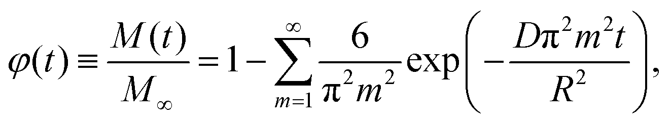 | (1) |
 | (2) |
 | (3) |
A more universal empirical expression for φ is
| φ = 1 − exp(−Btα), | (4) |
The most frequently applied empirical power-law expression attributed often in the area under consideration to Korsmeyer and Peppas13 is obtained by the linear expansion of (4) at Btα ≪ 1,
| φ = Btα. | (5) |
Often, the drug release can be limited by carrier dissolution and/or erosion. For spherically-shaped homogeneous carriers, the simplest shrinking core model describing this case predicts (see, e.g., ref. 14)
| φ = 1 − (R − vt)3/R3, | (6) |
In the literature, one can find many other models extending and/or complementing those mentioned above. In particular, diffusion-limited release was widely analyzed from various perspectives. Many treatments were aimed at the situations when the diffusion is Fickian whereas a carrier is either uniform but non-spherical15,16 or spherically shaped but with a uniform core and one or a few uniform shells.17–21 There are treatments22–25 aimed at explaining why the experimentally obtained exponent in (5) is often not equal to that of ≃0.5, expected in the case of Fickian diffusion [eqn (2)]. The focus is there on the non-Fickian diffusion related to the carrier structural heterogeneity on the length scale much smaller than the carrier size, e.g., due to the fractal-like carrier structure. The interplay of Fickian diffusion and carrier dissolution and/or erosion26–28 and the release after rupture of carrier particles29 were analyzed as well.
Regarding the comparison of theoretical and experimental release kinetics, one can note that the models usually imply that the size or initial size of carrier particles is fixed whereas in reality the kinetics are customarily measured at the ensemble level and represent convolution of the kinetics corresponding to the size distribution. From this perspective, the observed kinetics and/or obtained parameters are apparent and may be different compared to those corresponding to the fixed size. This effect may be important if the size distribution is appreciable16 as happens e.g. in the case of LNPs.
Taken together, the analytical expressions used to interpret and/or fit the measured release kinetics are either empirical or imply diffusion limitations of cargo and/or dissolution of carrier. Physically, the diffusion limitations take place provided the release of molecules located near the carrier–solution interface is sufficiently fast compared to diffusion inside a carrier on the length scale comparable to the carrier size.
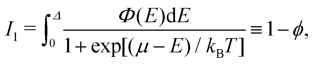
In the case of nanocarriers, the condition formulated above can be violated because the corresponding size is small (often ∼100 nm) and accordingly the diffusion timescale is short. An additional reason why this condition can fail in this limit is that the surface of nanoparticles is often well ordered and accordingly the release of molecules located near the carrier–solution interface may be slower compared to the diffusion inside. In the case of LNPs, for example, the carrier–solution interface typically represents a well-formed lipid bilayer.30–32 Under such circumstances, the diffusion limitations can be negligible at least sometimes, and the release can occur in the kinetically-limited regime. Another important factor is that biologically-relevant nanocarriers are often highly heterogeneous inside on the length scale much smaller than their size. For example, the poorly ordered internal part of LNPs (i) can be reminiscent of multilamellar vesicles with solution and RNA located between lipid leaflets30 or (ii) exhibit more complex and less ordered domains of the “cubic” phase, formed by a lipid bilayer and containing water channels31 or (iii) an “inverse hexagonal” phase.32 The structural heterogeneity of such carriers is expected to result in the complexity of the network of local minima and transition states at the potential-energy landscape for diffusion and release of molecules transported by a carrier. The distributions of energies of these local minima and transition states can be relatively broad. In other words, such carriers are expected to exhibit appreciable energetic heterogeneity. In the available kinetic models focused on diffusion limitation (e.g., ref. 22–25), as mentioned above, the structural heterogeneity is sometimes taken into account whereas the energetic heterogeneity is ignored.
Referring to nanocarriers, I present herein an alternative generic model implying kinetically limited release in the presence of appreciable energetic heterogeneity. This heterogeneity is described at the level of the already mentioned distributions of energies of local minima and transition states available at the potential energy surface (Section II). The diffusion of transported molecules inside a carrier is considered to be rapid (this condition corresponds to kinetically limited release) so that their distributions over sites is close to canonical. Despite this physical simplification, the corresponding general kinetic equations are rather cumbersome (Section II.A). In some practically important situations, they can be mathematically simplified (Section II.B) and used to illustrate the special features of the kinetics under consideration (Section III) and to discuss the relation of the results presented to what is observed in real systems (Sections IV and V).
II. Model
A. General equations
In the model under consideration, the local minima at the potential-energy landscape for the location of drug or vaccine molecules inside a carrier are identified with sites, and a carrier is viewed as a set of sites. Each site can be occupied by one molecule, and the corresponding energy of a molecule is designated as E. As mentioned in the introduction, carriers are assumed to be energetically heterogeneous, i.e., there is distribution of E designated as F(E). The minimal and maximal energies are identified with 0 and Δ. With this specification, E represents the deviation of energy from the minimal value. The E distribution is normalized as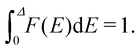 | (7) |
 | (8) |
In practically important cases, the number of molecules in a carrier is usually large (≫1), and accordingly the canonical distribution can be replaced by the grand canonical distribution,
 | (9) |
 | (10) |
| n = Nf, | (11) |
| N = V/v | (12) |
| N = 4πR3/3v, | (13) |
The carrier volume per site, v, is introduced above formally viaeqn (12) for N, i.e., it can be read as v = V/N and considered as the definition of v. In other words, a carrier is considered to be formed of sites, and the total volume of sites is equal to the carrier volume. The so-defined volume per site, v, is usually appreciably larger than the geometrical volume of a molecule.
The release of molecules from a carrier is considered to occur from some of the sites located near the carrier–solution interface. These sites form a subset of the whole set of sites, and the corresponding energy E of a molecule can also be in the range from 0 to Δ. As usual in the Arrhenius framework, the release is described in terms of the transition of a molecule along the potential energy surface so that E corresponds to the local minimum. The rate constant of release depends on E and also on the energy of a molecule in the activated state or, more specifically, on the deviation of this energy from the minimal value. Designating this deviation as E*, the release rate constant is represented as
k(E, E*) = ko![[thin space (1/6-em)]](https://www.rsc.org/images/entities/char_2009.gif) exp[−(E*−E)/kBT], exp[−(E*−E)/kBT], | (14) |
 . By definition,
  is the fraction of sites with the parameters in the ranges from E to E + dE and from E* to E* + dE*, and the corresponding normalization is as follows
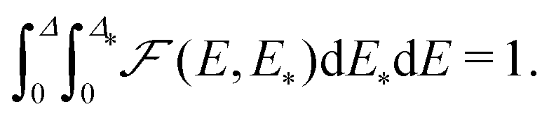 | (15) |
 | (16) |
 | (17) |
 | (18) |
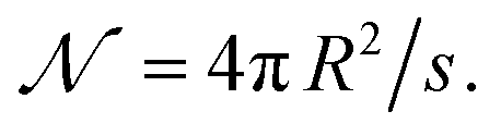
By analogy with the definition of v in eqn (12) and (13), s has been introduced above formally, i.e., eqn (17) can be read as  and considered as the definition of s. Regarding s, I can add that the carrier structure near the interface is typically different compared to that inside. In addition, not all the sites located at the interface are expected to allow release. For these reasons, the formally defined s can be appreciably larger than the average cross-sectional area of a site inside the carrier. With this reservation, s is expected to be much smaller than S.
The kinetic equation for release is
| dn/dt = −w. | (19) |
 | (20) |
 | (21) |
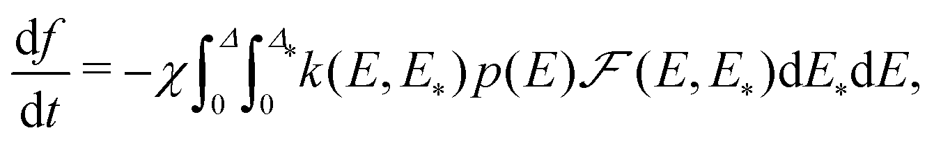
Eqn (20) for f in combination with (9), (10), and (14) for p(E), f, and k(E, E*) describes the release kinetics in the model under consideration. The right-hand part of this equation depends on f implicitly via the dependence of p(E) on f [eqn (9) and (10)]. According to eqn (20), the shape of the release kinetics is determined by the shapes of the distributions F(E) and  . For the timescale of release, the model yields
| τ ∝ 1/χ ∝ V/S. | (22) |
| τ ∝ R. | (23) |
Regarding χ in the equations above, I can add that biologically-relevant nanocarriers can usually be classified as soft matter, and with the release of cargo their size (or volume) and structure can change. The analysis of such changes is interesting from various perspectives. In the context under consideration, this means that χ can change with increasing time. If the heterogeneity of nanocarriers is appreciable (as assumed in my analysis), its effect on the release kinetics is expected to be much stronger than that of the change of χ. In addition to the heterogeneity itself, one of the arguments in this favour is that the total volume of molecules transported by a nanocarrier is often appreciably smaller than that of molecules forming a nanocarrier, and the changes of the size of a nanocarrier are frequently not expected to be dramatic. For these reasons, all the structural parameters, R, V, v, S, and s, used in the model are considered to be independent of time, and accordingly χ is independent of time as well. Physically, as already articulated, χ with its specification via V, v, S, and s is of interest in the context of carrier geometry and scaling issues [e.g., eqn (23)]. It does not, however, influence the shape of the release kinetics. Below, the presentation is focused on this shape, and accordingly χ is considered just as a model parameter.
B. Simplifications
In combination with (9), (10), and (14), eqn (20) is cumbersome. To facilitate its applications and understanding of the kinetics predicted, it makes sense to use three physically reasonable simplifications which may work although not always [in the latter case, one should use eqn (20)].First, one can expect that the correlation in the distribution of E and E* is often not of central importance, and in such cases this distribution can be factorized,
 | (24) |
| df/dt = −χkoI1I2exp(μ/kBT), | (25) |
 | (26) |
 | (27) |
| df/dt = −χko(1 − ϕ)exp(μ/kBT). | (28) |
The role of the energetic heterogeneity is appreciable if the distribution F(E) is broad. Such situations are of interest in the context of this study. In this limit, the dependence of the exponential term in eqn (25) on f is much stronger than that of 1 − ϕ, and accordingly 1 − ϕ can be safely replaced by 1 − f [this replacement is fully correct provided F(E) = Φ(E)]. With this (second) simplification, eqn (28) is modified as
| df/dt = −χko(1 − f)exp(μ/kBT). | (29) |
Regarding eqn (28) and (29), I can repeat that they are valid provided factorization (24) of  . In this case, the role of the E* distribution is reduced to the change of the timescale of the release, and it does not influence the shape of the kinetics. This case is sufficient in order to illustrate below the main special features of the kinetics under consideration. For more special goals, one can employ eqn (20) in combination with (9), (10), and (14).
If the distribution F(E) is narrow and can be neglected, the dependence of μ on f is well known to be
μ = kBT![[thin space (1/6-em)]](https://www.rsc.org/images/entities/i_char_2009.gif) ln[f/(1 − f)]. ln[f/(1 − f)]. | (30) |
| df/dt = −χkof. | (31) |
 | (32) |
 | (33) |
 | (34) |
III. Results of calculations
The specifics of the kinetics predicted by the model under consideration can be illustrated by employing the simplest uniform E distribution,| F(E) = 1/Δ. | (35) |
| μ = fΔ, | (36) |
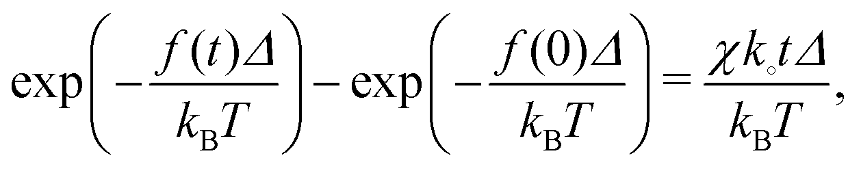
| df/dt = −χko(1 − f)exp(fΔ/kBT). | (37) |
In the situations of interest, the distribution F(E) is broad (Δ ≫ kBT). In this limit, as already indicated, the dependence of the exponential term in eqn (37) on f is much stronger than that of 1 − f, and accordingly 1 − f can be dropped in order to explain the key features of the kinetics, i.e., eqn (37) can be simplified,
| df/dt ≃ −χkoexp(fΔ/kBT), | (38) |
 | (39) |
 | (40) |
If 1 − f is kept in eqn (37), it can be integrated numerically. The corresponding results are presented in Fig. 1. In particular, Fig. 1(a) shows the release kinetics for Δ/kBT = 10 and f(0) = 0.3, 0.5, and 0.7. With increasing f(0), the number of sites involved in the release increases, the range of E corresponding to these sites increases as well, and accordingly the time interval corresponding to the transition from the linear to logarithmic kinetics becomes shorter. The kinetics for f(0) = 0.5 and Δ/kBT = 7, 10, and 13 are exhibited in Fig. 1(b). Here, the time interval corresponding to the transition from the linear to logarithmic kinetics becomes shorter with increasing Δ/kBT. This is further illustrated [Fig. 1(c)] by using a very wide energy distribution with Δ/kBT = 20. In this case, the initial phase of the kinetics (up to φ = 0.4) is very rapid and appears to be apparently stepwise.
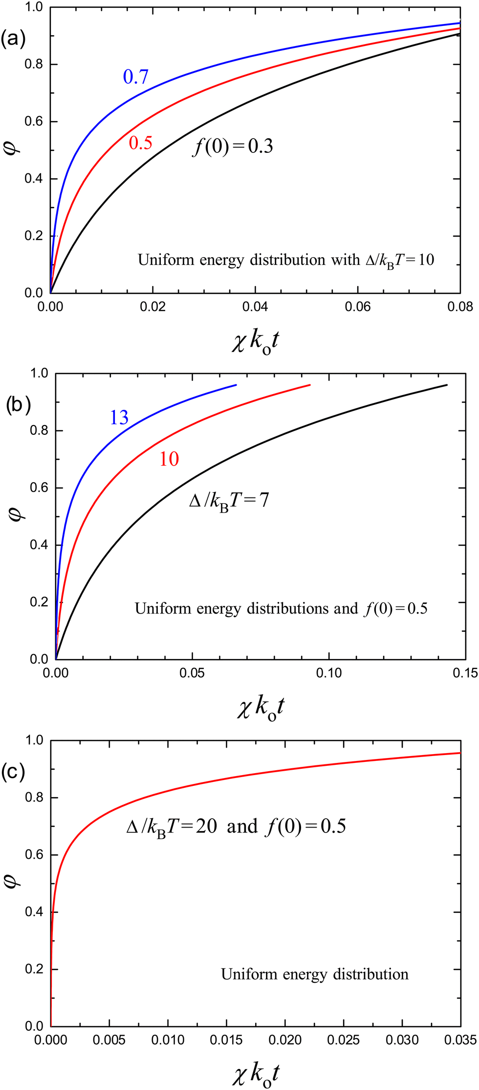 | ||
| Fig. 1 Kinetics of release of molecules from a carrier according to eqn (37) in the case of uniform distribution of sites over energy [eqn (35)] for (a) Δ/kBT = 10 and f(0) = 0.3, 0.5, and 0.7; (b) f(0) = 0.5 and Δ/kBT = 7, 10, and 13; and (c) f(0) = 0.5 and Δ/kBT = 20. | ||
The linearly-increasing or decreasing E distribution can be represented as
 | (41) |
 | (42) |
| μ = {A/2 − [A2/4 + (1 − A)f]1/2}Δ/(A − 1). | (43) |
The release kinetics calculated by using eqn (29) in combination with (43) are presented in Fig. 2 for f(0) = 0.5, Δ/kBT = 10, and A = 0.7, 1, and 1.3. Here, with increasing A, the range of E corresponding to the sites involved in the release decreases, and the time interval corresponding to the transition from the linear to logarithmic kinetics becomes longer.
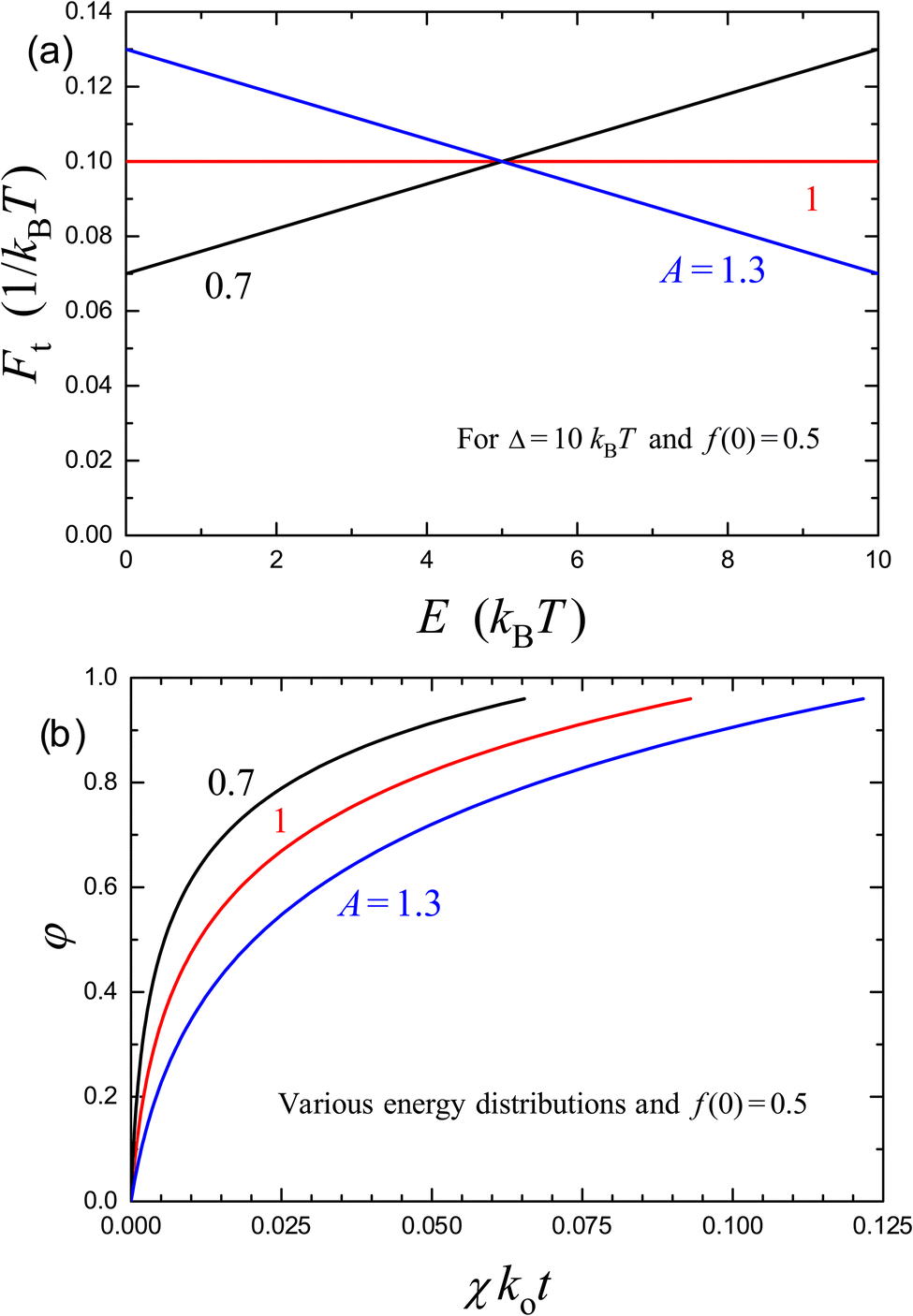 | ||
| Fig. 2 (a) Monotonously increasing, uniform, and monotonously decreasing distributions of site energies [eqn (41) with Δ/kBT = 10 and A = 0.7, 1, and 1.3, respectively], and (b) the corresponding kinetics of release of molecules from a carrier for f(0) = 0.5 according to eqn (29) in combination with (43). | ||
To link the results presented with those available in the literature, the two kinetics shown in Fig. 2 (for A = 0.7 and 1.3) have been fitted (Fig. 3) by employing the Weibull expression [eqn (4)]. The fit is nearly perfect in the whole range of φ provided the exponent α is set to 0.60 and 0.72, respectively. In fact, the difference between the curves is smaller than the typical error bar in the corresponding experimentally measured kinetics (for the latter, see e.g. Section IV below). Thus, the model proposed and the Weibull expression are formally equivalent in the context of fitting the experimentally observed kinetics. The Weibull expression is, however, axiomatic, whereas the model proposed can help to clarify the physics of the systems under consideration.
 | ||
| Fig. 3 Fit of the two kinetics shown in Fig. 2(b) with A = 0.7 (a) and 1.3 (b) by using the Weibull expression [eqn (4)] with α = 0.6 and 0.72, respectively. | ||
The conclusions above are applicable also to the fit by the Korsmeyer–Peppas expression [eqn (5)] which can be obtained by expansion of the Weibull expression and accordingly can safely be used provided φ is not too close to unity. In the whole range of φ, the accuracy of the Korsmeyer–Peppas expression is somewhat worse compared to that of the Weibull expression. Regarding this aspect, I can add that in experiments the range of φ is typically somewhat smaller than that shown in Fig. 3. One of the reasons might be that due to the logarithmic slowdown the kinetics cannot always be tracked up to φ = 1. In such situations, the accuracy of the Korsmeyer–Peppas expression is somewhat better. If the time interval in the model kinetics shown in Fig. 3 is reduced, their fit by employing the Korsmeyer–Peppas expression provides α values slightly smaller or larger than those corresponding to the Weibull expression. Concerning the obtained exponents, α = 0.60 and 0.72, I can add that the two kinetics shown in Fig. 2 and used for fitting in Fig. 3 were calculated with Δ/kBT = 10. With increasing Δ/kBT, α will be smaller.
The fact that the kinetics predicted by the model under consideration can be well fitted by using the Weibull or Korsmeyer–Peppas expression (Fig. 3) is a consequence of the choice of the energy distributions which are relatively broad and monotonous. The corresponding kinetics (Fig. 2 and 3) have been calculated by using eqn (29) in combination with (43). The model in its general form [eqn (20) in combination with (9), (10), and (14)] or more simple eqn (29) in combination with (10) or (33) are applicable to other energy distributions as well.
For example, the simplest alternative distribution is that for sites of two types with energies E1= 0 and E2 = Δ, so that eqn (10) is reduced to
 | (44) |
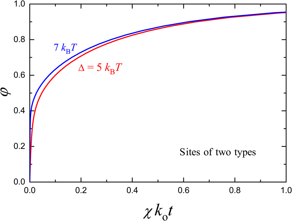 | ||
| Fig. 4 Kinetics of the release of molecules from a carrier containing absorption sites of two types with E1 = 0 and E2 = Δ, according to eqn (29) and (44) with f(0) = 0.8, θ1 = θ2 = 0.5, and Δ = 5 and 7kBT. In both cases, the initial phase of the kinetics (up to φ = 0.4) is very rapid. For Δ = 7kBT, this phase is apparently stepwise [as in Fig. 1(c)]. These kinetics are poorly fitted by the Weibull and Korsmeyer–Peppas expressions. | ||
Of note, the logarithmic kinetics related to a broad distribution of kinetic parameters were previously experimentally observed and theoretically analyzed in various branches of natural sciences. For example, I refer to the studies focused on the kinetics of adsorption on and desorption from heterogeneous surfaces with distribution of binding and activation energies,33 electron transport in nanocrystalline semiconductor films,34 and electron tunneling at low temperatures in arrays of immobile donors and acceptors or arrays of donors–acceptor pairs with appreciable distribution of distances between donors and acceptors.35 To some extent, the description of adsorption on and desorption from heterogeneous surfaces is similar to what I present. The difference is that these processes occur exclusively at surface sites, whereas the release under consideration occurs from the sites located near the interface and the occupation of these sites is, in fact, dictated by the occupation of sites located inside a carrier. For this reason, the details of the math are different. For instance, the key general equation derived in my work is (20). I have simplified it down to (37) for the calculations shown in Fig. 1. For qualitative illustration, I have further simplified (37) down to (38). The latter equation is e.g. similar (except the sign and designations) to eqn (1) presented in ref. 33 for describing the kinetics of adsorption. The corresponding kinetics (eqn (40) in my case and eqn (2) in ref. 33) exhibit similar logarithmic features.
IV. Related experimental results
Regarding the comparison of the model predictions with the results of available experiments, I can repeat (cf. the introduction) that the Weibull and Korsemeyer–Peppas expressions were/are very widely employed for fitting the observed release kinetics. Many suitable examples can be found with the corresponding references e.g. in the review published in 2019 by Mircioiu et al.7 (see Tables 1, 2 and 4 for micro- and nano-sized carriers). The range of the exponents collected there is rather large, 0.45 ≤ α ≤ 0.85.Aiming at more recent experiments, one can employ “Korsmeyer–Peppas” as search words in e.g. Sci. Cit. Ind. It yields a few hundred examples of the use of the corresponding expression for fitting the observed kinetics of release from various carriers. Several relevant recent studies (ref. 36–47) reporting typical values of α are as follows.
Alinavaz et al.36 explored magnetic carboxymethylcellulose/chitosan bio-nanocomposites of ∼50 nm size for smart co-delivery of sunitinib malate anticancer compound and saffron extract. α is reported to be in the range from 0.30 to 0.60.
Altoom et al.37 used cellulose fibers/zeolite-A biocomposites of ∼100–200 nm size as a carrier of oxaliplatin drug. α is reported to be in the range from 0.53 to 0.70.
Ge et al.38 studied magadiite-sodium alginate drug carrier composites of different shapes and sizes. α is reported to be in the range from 0.40 to 0.66.
Gilani et al.39 explored osimertinib nano lipid carriers of ∼150 nm size. α is reported to be 0.43.
Haseli et al.40 used release of curcumin from chitosan-based carriers of ∼100 nm size. α is reported to be 0.78 and 1.01.
Luo et al.41 explored sorafenib-loaded LNPs of ∼100 nm size for in vitro and in vivo studies in the context of topical ocular therapy of corneal neovascularization. α is reported to be 0.44 and 0.97.
Ozkahraman et al.42 employed N-vinylcaprolactam and methacrylic acid based hydrogels (with the heterogeneity on the scale of ∼1 μm) in the context of drug release. α is reported to be in the range from 0.40 to 0.56.
Qiao et al.43 used silk fabric decorated with hydrogel (with the heterogeneity on the scale up to ∼10 μm) for sustained release of paracetamol. α is reported to be 0.66 and 0.68.
Truong et al.44 employed ∼150 nm-sized LNPs as carriers for Capsicum oleoresin. α is reported to be 0.86.
Truong et al.45 also used ∼250 nm-sized chitosan-coated LNPs for transdermal delivery of tetrahydrocurcumin. α is reported to be 0.36 and 0.66.
Velez-Pena et al.46 employed mesoporous mixed oxides of ∼700–1100 nm size as drug delivery carriers for methotrexate. α is reported to be in the range from 0.49 to 0.62.
Yildirim and Dogac47 studied the release of 5-fluorouracil from magnetic MnFe2O4/alginate beads in the context of cancer drug delivery. α is reported to be in the range from 0.43 to 62.
In agreement with the previous studies reviewed by Mircioiu et al.,7 recent studies (ref. 36–47) focused on various cargos and carriers show that α is often in the range from 0.45 to 0.85. As I have illustrated in Section III, the Weibull and Korsemeyer–Peppas expressions with this range of α can easily be reproduced by using the model under consideration with appreciable heterogeneity. Thus, this model can be used to fit numerous experimentally measured kinetics and the fit will obviously good. This means that the model is formally applicable to the corresponding real systems and can be potentially applicable to many other systems.
V. Conclusions
The kinetics of drug or vaccine release from carriers are of high interest from various perspectives. With decreasing the carrier size down to ∼100 nm and using the biologically-inspired soft-matter carriers, the timescale of diffusion of drug or vaccine molecules is shortened, and the release kinetics are likely to be kinetically limited. I have presented the generic kinetic model describing this regime of release and allowing one to take the energetic heterogeneity into account (Section II). In the absence of heterogeneity, the model is reduced to the first-order equation resulting in exponential kinetics. In the calculations illustrating the effect of heterogeneity on the corresponding kinetics (Section III), the deviation of the molecule binding from the minimal value was considered to be ∼7–13kBT (4–8 kcal mol−1). Roughly, this is about one third or fourth of the likely activation barrier for release. With this physically reasonable (for non-covalent interaction) scale of heterogeneity, the predicted kinetics (i) are linear in the very beginning and then, with increasing time, become logarithmic and (ii) can be nearly perfectly fitted by using the empirical Weibull or Korsmeyer–Peppas expressions with the exponent α in the range from 0.6 (or somewhat lower) to 0.75. Taken together, the result obtained (Section III) indicates that in terms of the conventional empirical expressions the kinetics predicted by model I use can formally be characterized by α in the range from 0.6 (or somewhat lower) to 1. The values of α obtained here for energetically heterogeneous carriers [from 0.6 (or somewhat lower) to 0.75] are usually associated with non-Fickian diffusion. The model presented shows that the energetic heterogeneity can be operative in these cases as well.The range of the values of α predicted by the model under consideration is in agreement with that observed in experiments (Section IV). From this perspective, the model is practically relevant. Whether or not the model is really applicable and whether or not it is preferable compared to the other available models should be clarified e.g. by exploring the specifics of the structure of micro- or nanocarriers and simultaneously measuring the rate of diffusion of drug or vaccine molecules inside and comparing the diffusion time scale with that of release. Such measurements are challenging and now lacking (see, e.g., the already mentioned recent studies36–47).
Regarding the applicability of the model to the biologically-inspired soft-matter nanocarriers, one should bear in mind that it operates with a fixed number of sites and distributions of energies of molecules bound at sites. Soft-matter nanocarriers (e.g., LNPs) are expected to be dynamic and the number of sites and distributions of sites over energy can vary in the course of release. The model is applicable provided the corresponding variations are modest.
The model does not take the interaction between molecules into account. At the mean-field level, this interaction is well known to be described by introducing the linear term, Cf (C is a constant proportional to the interaction energy), into the chemical potential. If needed, this modification can easily be incorporated into the equations presented in Sections II and III. Often, this is a matter of redefinition of some of the parameters. At a higher level, the inclusion of the interaction between molecules should be made in parallel with that of the correlation between the location of sites with different energies, and it results in cumbersome equations which can be analyzed only numerically.
Finally, I add two general remarks in order to extend slightly the scope of the discussion above:
(i) The kinetic models briefly outlined in the introduction were originally proposed primarily in the context of drug release from macroscopic pellets. The model treated in my work has been motivated by referring to biologically-inspired nanocarriers. It is expected to be applicable to experiments performed both in vitro and in vivo. The situations in vivo can be much richer than those described by the models mentioned. For example, the intracellular release from LNPs may occur during their interaction with lipid membranes (e.g., at anionic membranes of endosomes). The corresponding concepts are now available48,49 whereas the suitable kinetic models are lacking in fact (see e.g. the discussion in ref. 29).
(ii) With minor modifications the treatment presented in this study can be used to describe systems which were not mentioned above. In nanoscience, for example, the release of hydrogen from alloyed metal nanoparticles attracts nowadays attention from various perspectives.50 In the context of hydrogen absorption, such particles are energetically heterogeneous. The H2 release occurs via associative desorption of hydrogen from the surface, whereas the hydrogen surface coverage is controlled by hydrogen absorbed inside. The corresponding absorption isotherms have already been analyzed theoretically,51 whereas the treatment of the release kinetics taking the heterogeneity into account is still lacking. With some modifications, it can be done by using the formalism presented.
Conflicts of interest
There are no conflicts to declare.Acknowledgements
The author thanks Prof. F. Höök for useful discussions. The work was supported by the Ministry of Science and Higher Education of the Russian Federation within the governmental order for Boreskov Institute of Catalysis (project AAAA-A21-121011390008-4).References
- S. Agrawal, J. Fernandes, F. Shaikh and V. Patel, Quality aspects in the development of pelletized dosage forms, Heliyon, 2022, 8, e08956 CrossRef CAS PubMed.
- M. S. Handattu, S. Thirumaleshwar, G. M. Prakash, H. K. Somareddy and G. H. Veerabhadrappa, A comprehensive review on pellets as a dosage form in pharmaceuticals, Curr. Drug Targets, 2021, 22, 1183–1195 CrossRef CAS PubMed.
- T. Chen, J. Li, T. Chen, C. C. Sun and Y. Zheng, Tablets of multi-unit pellet system for controlled drug delivery, J. Controlled Release, 2017, 262, 222–231 CrossRef CAS PubMed.
- M. J. Mitchell, M. M. Billingsley, R. M. Haley, M. E. Wechsler, N. A. Peppas and R. Langer, Engineering precision nanoparticles for drug delivery, Nat. Rev. Drug Discovery, 2021, 20, 101–124 CrossRef CAS PubMed.
- X. Hou, T. Zaks, R. Langer and Y. Dong, Lipid Nanoparticles for mRNA delivery, Nat. Rev. Mater., 2021, 6, 1078–1094 CrossRef CAS PubMed.
- J. A. Jackman, et al., Antiviral therapies and vaccines, Adv. Funct. Mater., 2020, 31, 2008352 CrossRef.
- C. Mircioiu, et al., Mathematical modeling of release kinetics from supramolecular drug delivery systems, Pharm., 2019, 11, 140 CAS.
- N. A. Peppas and B. Narasimhan, Mathematical models in drug delivery: How modeling has shaped the way we design new drug delivery systems, J. Controlled Release, 2014, 190, 75–81 CrossRef CAS PubMed.
- J. Siepmann and F. Siepmann, Modeling of diffusion controlled drug delivery, J. Controlled Release, 2012, 161, 351–362 CrossRef CAS PubMed.
- A. Hadjitheodorou and G. Kalosakas, Quantifying diffusion-controlled drug release from spherical devices using Monte Carlo simulations, Mater. Sci. Eng., C, 2013, 33, 763–768 CrossRef CAS PubMed.
- W. Weibull, A statistical distribution function of wide applicability, ASME J. Appl. Mech., 1951, 293–297 CrossRef.
- V. Papadopoulou, K. Kosmidis, M. Vlachou and P. Macheras, On the use of the Weibull function for the discernment of drug release mechanisms, Int. J. Pharm., 2006, 309, 44–50 CrossRef CAS PubMed.
- R. W. Korsmeyer, R. Gumy, E. Doelker, P. Buri and N. A. Peppas, Mechanisms of solute release from porous hydrophilic polymers, Int. J. Pharm., 1983, 15, 25–35 CrossRef CAS.
- J. Siepmann and F. Siepmann, Mathematical modeling of drug dissolution, Int. J. Pharm., 2013, 453, 12–24 CrossRef CAS PubMed.
- K. Kosmidis, P. Argyrakis and P. Macheras, A reappraisal of drug release laws using Monte Carlo simulations: the revalence of the Weibull function, Pharm. Res., 2003, 20, 988–995 CrossRef CAS PubMed.
- T. I. Spiridonova, S. I. Tverdokhlebov and Y. G. Anissimov, Investigation of the size distribution for diffusion-controlled drug release from drug delivery systems of various geometries, J. Pharm. Sci., 2019, 108, 2690–2697 CrossRef CAS PubMed.
- E. J. Carr and G. Pontrelli, Modelling mass diffusion for a multi-layer sphere immersed in a semi-infinite medium: application to drug delivery, Math. Biosci., 2018, 303, 1–9 CrossRef CAS PubMed.
- E. J. Carr and G. Pontrelli, Drug delivery from microcapsules: How can we estimate the release time?, Math. Biosci., 2019, 315, 108216 CrossRef CAS PubMed.
- G. Pontrelli, E. J. Carr, A. Tiribocchi and S. Succi, Modeling drug delivery from multiple emulsions, Phys. Rev. E, 2020, 102, 023114 CrossRef CAS PubMed.
- A. Jain, S. McGinty, G. Pontrelli and L. Zhou, Theoretical model for diffusion-reaction based drug delivery from a multilayer spherical capsule, Int. J. Heat Mass Transfer, 2022, 183, 122072 CrossRef CAS.
- S. Mubarak and M. A. Khanday, Mathematical modelling of drug-diffusion from multi-layered capsules/tablets and other drug delivery devices, Comput. Meth. Biomech. Biomed. Eng., 2022, 25, 896–907 CrossRef PubMed.
- P. Macheras and A. Dokoumetzidis, On the heterogeneity of drug dissolution and release, Pharm. Res., 2000, 17, 108–112 CrossRef CAS PubMed.
- K. Kosmidis and P. Macheras, Monte Carlo simulations for the study of drug release from matrices with high and low diffusivity areas, Int. J. Pharm., 2007, 343, 166–172 CrossRef CAS PubMed.
- P. D. Mavroudis, K. Kosmidis and P. Macheras, On the unphysical hypotheses in pharmacokinetics and oral drug absorption: time to utilize instantaneous rate coefficients instead of rate constants, Eur. J. Pharm. Sci., 2019, 130, 137–146 CrossRef CAS PubMed.
- J. A. Maroto-Centeno and M. Quesada-Perez, Coarse-grained simulations of diffusion controlled release of drugs from neutral nanogels: effect of excluded volume interactions, J. Chem. Phys., 2020, 152, 024107 CrossRef CAS PubMed.
- V. P. Zhdanov, Intracellular RNA delivery by lipid nanoparticles: diffusion, degradation, and release, BioSystem, 2019, 185, 104032 CrossRef PubMed.
- A. Jain, S. McGinty and G. Pontrelli, Drug diffusion and release from a bioerodible spherical capsule, Int. J. Pharm., 2022, 616, 121442 CrossRef CAS PubMed.
- M. S. Gomes-Filho, F. A. Oliveira and M. A. A. Barbosa, Modeling the diffusion-erosion crossover dynamics in drug release, Phys. Rev. E, 2022, 105, 044110 CrossRef CAS PubMed.
- V. P. Zhdanov, Lipid nanoparticles with ionizable lipids: statistical aspects, Phys. Rev. E, 2022, 105, 044405 CrossRef CAS PubMed.
- M. A. Oberli, et al., Immunotherapy, Nano Lett., 2017, 17, 1326–1335 CrossRef CAS PubMed.
- S. S. W. Leung and C. Leal, The stabilization of primitive bicontinuous cubic phases with tunable swelling over a wide composition range, Soft Matter, 2019, 15, 1269–1277 RSC.
- N. Y. Arteta, et al., Successful reprogramming of cellular protein production through mRNA delivered by functionalized lipid nanoparticles, Proc. Natl. Acad. Sci. U. S. A., 2018, 115, E3351–E3360 Search PubMed.
- I. S. McLintock, The Elovich equation in chemisorption kinetics, Nature, 1967, 216, 1204–1205 CrossRef CAS.
- J. Nelson, Continuous-time random-walk model of electron transport in nanocrystalline TiO2 electrodes, Phys. Rev. B: Condens. Matter Mater. Phys., 1999, 59, 15374–15380 CrossRef CAS.
- R. F. Khairutdinov, K. I. Zamaraev and V. P. Zhdanov, Electron Tunneling in Chemistry, Elsevier, Amsterdam, 1989 Search PubMed.
- S. Alinavaz, et al., Novel magnetic carboxymethylcellulose/chitosan bio-nanocomposites for smart co-delivery of sunitinib malate anticancer compound and saffron extract, Polym. Intern., 2022, 71, 1243–1251 CrossRef CAS.
- N. Altoom, et al., Insight into the loading, release, and anticancer properties of cellulose/zeolite-A as an enhanced delivery structure for oxaliplatin chemotherapy; characterization and mechanism, J. Sol-Gel Sci. Technol., 2022, 103, 752–765 CrossRef CAS.
- M. Ge, et al., Preparation of magadiite-Sodium alginate drug carrier composite by pickering-emulsion-templated-encapsulation method and its properties of sustained release mechanism by Baker-Lonsdale and Korsmeyer-Peppas model, J. Polym. Environ., 2022, 30, 3890–3900 CrossRef CAS.
- S. J. Gilani, et al., Formulation of osimertinib nano lipid carriers: optimization, characterization and cytotoxicity assessment, J. Cluster Sci., 2023, 34, 1051–1063 CrossRef CAS.
- S. Haseli, et al., A novel pH-responsive nanoniosomal emulsion for sustained release of curcumin from a chitosan-based nanocarrier: Emphasis on the concurrent improvement of loading, sustained release, and apoptosis induction, Biotechnol. Prog., 2022, 38, e3280 CrossRef CAS PubMed.
- Q. Luo, et al., Sorafenib-loaded nanostructured lipid carriers for topical ocular therapy of corneal neovascularization: development, in-vitro and in vivo study, Drug Delivery, 2022, 29, 837–855 CrossRef CAS PubMed.
- B. Özkahraman, I. Acar and G. Guclu, Synthesis of N-vinylcaprolactam and methacrylic acid based hydrogels and investigation of drug release characteristics, Polym. Bull., 2023, 80, 5149–5181 CrossRef.
- N. Qiao, et al., Silk fabric decorated with thermo-sensitive hydrogel for sustained release of paracetamol, Macromol. Biosci., 2022, 2200029 CrossRef CAS PubMed.
- C. T. Truong, et al., Development of topical gel containing Capsicum oleoresin encapsulated Tamanu nanocarrier and its analgesic and anti-inflammatory activities, Mater. Today Commun., 2022, 31, 103404 CrossRef CAS.
- T. H. Truong, et al., Chitosan-coated nanostructured lipid carriers for transdermal delivery of tetrahydrocurcumin for breast cancer therapy, Carbohydr. Polym., 2022, 288, 119401 CrossRef CAS PubMed.
- E. Velez-Pena, et al., Mesoporous mixed oxides prepared by hard template methodology as novel drug delivery carriers for methotrexate, J. Drug Deliv. Sci. Technol., 2022, 73, 103483 CrossRef CAS.
- A. Yildirim and Y. I. Dogac, MnFe2O4/alginate magnetic beads as platform for cancer drug delivery: an in vitro study of 5-fluorouracil release, J. Macromol. Sci. A Pure Appl. Chem., 2022, 59, 558–566 CrossRef CAS.
- S. A. Smith, L. I. Selby, A. P. R. Johnston and G. K. Such, The endosomal escape of nanoparticles: toward more efficient cellular delivery, Bioconjugate Chem., 2019, 30, 263–272 CrossRef CAS PubMed.
- I. M. S. Degors, C. Wang, Z. U. Rehman and I. S. Zuhorn, Carriers break barriers in drug delivery: endocytosis and endosomal escape of gene delivery vectors, Acc. Chem. Res., 2019, 52, 1750–1760 CrossRef CAS PubMed.
- F. A. A. Nugroho, et al., Metalpolymer hybrid nanomaterials for plasmonic ultrafast hydrogen detection, Nat. Mater., 2019, 18, 489–495 CrossRef CAS PubMed.
- M. Mamatkulov and V. P. Zhdanov, Partial or complete suppression of hysteresis in hydride formation in binary alloys of Pd with other metals, J. Alloys Compd., 2021, 885, 160956 CrossRef CAS.
| This journal is © the Owner Societies 2023 |