
 Open Access Article
 This Open Access Article is licensed under a Creative Commons Attribution-Non Commercial 3.0 Unported Licence
The roto-conformational diffusion tensor as a tool to interpret molecular flexibility†
Sergio
Rampino
 ,
Mirco
Zerbetto
* and
Antonino
Polimeno
,
Mirco
Zerbetto
* and
Antonino
Polimeno
Department of Chemical Sciences, University of Padova, Via Marzolo 1, I-35131, Padova, Italy. E-mail: mirco.zerbetto@unipd.it; Fax: +39 049 8275050; Tel: +39 049 8275678
First published on 12th May 2023
Abstract
Stochastic modeling approaches can be used to rationalize complex molecular dynamical behaviours in solution, helping to interpret the coupling mechanisms among internal and external degrees of freedom, providing insight into reaction mechanisms and extracting structural and dynamical data from spectroscopic observables. However, the definition of comprehensive models is usually limited by (i) the difficulty in defining – without resorting to phenomenological assumptions – a representative reduced ensemble of molecular coordinates able to capture essential dynamical properties and (ii) the complexity of numerical or approximate treatments of the resulting equations. In this paper, we address the first of these two issues. Building on a previously defined systematic approach to construct rigorous stochastic models of flexible molecules in solutions from basic principles, we define a manageable diffusive framework leading to a Smoluchowski equation determined by one main tensorial parameter, namely the scaled roto-conformational diffusion tensor, which accounts for the influence of both conservative and dissipative forces and describes the molecular mobility via a precise definition of internal–external and internal–internal couplings. We then show the usefulness of the roto-conformational scaled diffusion tensor as an efficient gauge of molecular flexibility through the analysis of a set of molecular systems of increasing complexity ranging from dimethylformamide to a protein domain.
1. Introduction
The dynamical behaviour of macromolecules in solution plays a key role in biological contexts. Dynamics is in fact responsible for generating a set of different structures of the same protein, for tuning binding properties of folded proteins (allosterism), for regulating pathways of folding and binding, and for controlling the function of disordered proteins or domains.1,2 Accessing and understanding molecular motion is thus of primary importance in the study of these processes. In this respect, a number of techniques have been developed over the years to investigate macromolecular dynamics, both from the experimental (e.g., NMR,3 fluorescence techniques,4 time-resolved X-ray scattering,5 atomic force microscopy,6 neutron spectroscopy;7 see this last reference for a comprehensive review) and the theoretical and computational perspectives. The dynamics of macromolecules in solution can in principle be reproduced in silico by fully atomistic molecular dynamics (MD) simulations through popular packages such as GROMACS, CHARMM and NAMD. However, considering a medium-size protein with a sufficient number of surrounding water molecules an order of 104–105 atoms is typically reached, and limitations due to computational cost both in terms of time and memory usage are easily met even on high-performance computing platforms. To overcome these limitations, several strategies can be pursued.First of all, direct coarse-grained approaches have been developed over the years with the aim of reducing the number of explicitly considered degrees of freedom by collecting in some appropriate way groups of atoms into collective particles (beads) and adopting an effective force field among them, also aided by state-of-the art machine-learning techniques.8,9 A less direct but intriguing approach is followed when distinguishing between relevant motions (or coordinates), primarily affecting the process or property under study, and non-relevant ones, which have – or are supposed to have – a negligible effect and can be treated in some suitable approximate way. This is the field of the so-called relevant dynamics: in other words, a few important details are supposed to be responsible for a phenomenon to happen, while all the others can be thought of as molecule-dependent fine tuners of the properties of the phenomenon. In these approaches, the problem is thus that of defining/finding the relevant coordinates of the system, focusing on the important, hopefully small, subset of degrees of freedom. The partition “relevant vs. irrelevant” can be based on purely phenomenological considerations, or, at least approximately, on algorithmic procedures. In the Gaussian Network Model, for instance, the molecule is seen as an ensemble of beads interacting within a cutoff radius with a harmonic potentials of the same strength.10,11 The diagonalization of the so-called Kirchoff matrix (worked out from the variance-covariance matrix describing the correlation between the displacements of bead pairs) leads to the definition of a set of generalized coordinates (linear combinations of Cartesian coordinates of the beads) whose relevance in terms of relaxation times is directly proportional to the amplitude of the motion given by the related eigenvalue. Similar alternative models are the anisotropic network model, based on the diagonalization of the Hessian of the potential instead of the Kirchoff matrix,12,13 and the normal mode analysis, expressing the dynamics of a protein as a superposition of collective motions called normal modes.14,15 Among other viable approaches, the filtering technique is based on the idea of removing high-frequency fast motions with a low pass filter applied to a Fourier transformed MD trajectory,16,17 to focus on the structural and energetic features of low-frequency collective motions. Singular Value Decomposition is thought to be very useful for characterization of the nonlinear dynamics of multivariate systems and to the identification of the dominant modes of motion in systems whose cooperative dynamics cannot be fully explored within reasonable computation time using conventional simulation techniques.18 Finally, the widely employed principal component analysis,19 also known as essential dynamics, involves as some of the previously mentioned techniques the construction and diagonalization of a matrix which leads to the definition of collective generalized coordinates.
Once defined, the subset of relevant coordinates can be described using stochastic approaches, which are particularly useful when discussing molecules in solutions. The definition of a comprehensive approach to define molecularly-based Fokker–Planck (FP) models can be conducted within a general framework. In our previous work20,21 we gave a contribution to the definition of a general procedure to derive a FP description by addressing the relaxation processes of a flexible (macro)molecule as a non-rigid body, based on a generic set of internal and external degrees of freedom, which define a Markovian process. This was pursued by first setting up the Liouville equation of motion22 for a generic flexible body defined as a set of material points (atoms or beads), in terms of roto-translational and natural internal coordinates. The general description of a macromolecule in solution was then carried out in terms of a collection of flexible bodies, to which a standard Nakajima-Zwanzig23,24 projection method was applied in order to eliminate the irrelevant, i.e. not directly observed, degrees of freedom. A generalized master equation was obtained. Alternative modeling options, based on different choices of the internal variables, of accuracy levels of the description of solvents effects, etc., were reviewed. The case of a partially rigid Brownian rotator (semi-flexible body model), i.e. with only internal modes described by a harmonic internal energy, was discussed.21
The resulting theoretical approach, while effective, is still considerably challenging from a computational point of view. To partially overcome this limitation, we propose here to simplify the general scheme20,21 by projecting out all the conjugate momenta. Such an approximation is valid in the diffusive limit, and leads to the Smoluchowski description of the stochastic motion of the relevant coordinates only. We present in particular in this paper first, for sake of completeness, the derivation of the diffusive description from the general model, and then we concentrate on the characteristics of the main tensorial parameter defining the resulting FP equation, i.e. the (scaled) roto-conformational diffusive tensor, D, which includes, at least for semi-flexible systems not undergoing large amplitude internal motions, information on both the molecular internal energy landscape and the dispersive medium. In particular, we intend to test the usefulness of D as a gauge of molecular flexibility. We argue that, by analysing in different ways the tensor elements, its eigenvalues spectrum and other derived quantities, it is possible to acquire additional insight into the molecular mobility. To do so, after sketching the theoretical framework in Section 2, we analyze in Section 3 the features of the roto-conformational diffusion tensor for molecular systems of increasing complexity, ranging from the simple dimethylformamide to a protein domain, and we discuss its possible role as a signature for measuring the dynamical relevance of subsets of coordinates. Conclusions are drawn in Section 4 and some perspectives are outlined.
2. Roto-conformational diffusive equation
Following ref. 20 and 21 (neglecting translational degrees of freedom) we can identify for a generic non-rigid molecule in a homogeneous medium a set of rotational coordinates (Ω) defined with respect to some convenient instantaneous molecular frame and the related angular momentum (L) as external variables, coupled with a set of internal generic coordinates and their momenta (q, p). A detailed summary of the basic hypotheses required to derive a complete non-Hermitian FP equation for the conditional probability of the system can be found in the ESI,† for the interested reader. From eqn (S1) of the ESI,† several sources of couplings can be observed: inertial coupling between coordinates and momenta, precession terms, kinetic coupling related to the generalized intertia tensor in the kinetic energy, friction coupling, i.e. dissipative forces resulting from the full friction tensor including non-zero roto-conformational blocks. All these quantities are shape dependent, i.e. they are defined by tensors, which are functions of q.This picture is somewhat simplified when a diffusive limit is considered, i.e. when it is assumed that momenta L, p relax much faster then positional coordinates Ω, q. This is a reasonable approximation, usually introduced when discussing molecular relaxation processes in normal fluids at room temperature. The original complete FP equation discussed in ref. 20 and 21, can be therefore simplified by the rigorous elimination (via projection) of the momenta, which are considered as fast relaxing modes. The resulting time evolution operator in the reduced configuration space Ω, q is Hermitian (or easily reduced to a Hermitian form), allowing for a considerably increased efficiency in the subsequent numerical treatment, without renouncing to the full inclusion of internal degrees of freedom, based on non-phenomenological assumptions. The procedure employed to project the momenta follows a standard Nakajima–Zwanzig23–25 formalism, and is sketched in the ESI† for the sake of completeness. The result is the diffusive (Smoluchowski) equation for the time dependent conditional probability ρ(x,t) with x = (Ω, q), obtained after averaging out all the momenta L, p
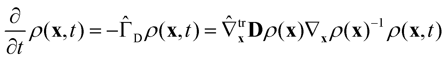 | (1) |
 | (2) |
 | (3) |
 | (4) |
 | (5) |
 | (6) |
3. Results
3.1 Systems
An ensemble of eight molecular systems of increasing complexity has been analyzed (see Fig. 1). The simplest system is dimethylformamide (DMF hereinafter), with 12 atoms and 30 internal degrees of freedom. Then follows a series of six oligosaccharides constituted by 2 to 8 sugar units, number of atoms ranging from 46 to 168, and number of internal degrees of freedom ranging from 132 to 498: | ||
| Fig. 1 Three-dimensional representations of the molecular structures of the eight considered systems. The three atoms defining the orientation reference frame (see text for discussion) are highlighted as spheres. | ||
• α-L-Rhap-α-(1 → 2)-α-L-Rhap-OMe (R2R, 2 residues)
• β-D-Glcp-(1 → 6)-α-D-[6-13C]-Manp-OMe (BGL, 2 residues)
• β-D-Glcp-(1 → 3)[β-D-Glcp-(1 → 2)]-α-D-Manp-OMe (GGM, 3 residues)
• α-D-Manp-(1 → 2)-α-D-Manp-(1 → 6)-α-D-[6-13 C]-Manp-OMe (TRI, 3 residues)
• α-L-Fucp-(1 → 2)-β-D-Galp-(1 → 3)-β-D-GlcpNAc-(1 → 3)-β-D-Galp-(1 → 4)-D-Glcp (LNF, 5 residues)
• γ-cyclodextrin (GCY, 8 residues)
The last (and most complex) considered system is GB3 protein (PDB id: 1P7F), with 56 amino acid residues, 862 atoms and 2580 internal degrees of freedom. The orientation of the molecular frame is defined by three consecutively bonded atoms as follows: the origin coincides with the position of the second atom, the first atom lies on the negative x axis, and the third atom lies in the xy plane. For DMF and for the oligosaccharides the first two atoms were selected as the hydrogen and the carbon, respectively, of a plausible NMR probe (either CH or CH2); for GB3 the triplet of atoms defining the orientation frame was chosen as the first three atoms (NCC) of the polymer backbone. Fig. 1 shows the molecular structures of the considered systems with the above mentioned triplets of atoms highlighted as spheres.
In the hydrodynamic model used to evaluate the friction tensor, four quantities are required, namely: the temperature, the local viscosity, the hydrodynamic boundary conditions and the effective radius of the atoms, Reff. For the set of oligosaccharides, temperature and viscosity were chosen among those for which experimental NMR data are available (see ref. 26–30), and Reff was set to the optimal value providing the lowest sum of squared percentage deviations for T1, T2 and NOE over the entire ensemble of experimental data available for each system, as estimated in ref. 31. For DMF and GB3, temperature and viscosity were arbitrarily chosen, and a value of Reff = 2.0 Å was used. For all systems stick boundary conditions were applied. A summary of the parameters used for all the considered systems is provided in Table 1. Calculations were performed according to the computational protocol described in the ESI.†
| DMF | R2R | BGL | GGM | TRI | LNF | GCY | GB3 | |
|---|---|---|---|---|---|---|---|---|
| T/K | 298.15 | 298.2 | 253.0 | 298.6 | 298.0 | 303.0 | 323.0 | 298.15 |
| η/cP | 2.19 | 2.19 | 2.82 | 1.09 | 3.66 | 1.40 | 2.90 | 0.91 |
| R eff/Å | 2.0 | 1.6 | 1.8 | 1.8 | 2.2 | 3.2 | 1.8 | 2.0 |
3.2 Rotational part of the diffusion tensor
In Table 2, the following three sets of values are reported for each systems in units of fs−1:| i = 1 | i = 2 | i = 3 | |
|---|---|---|---|
| DMF | |||
| D (RR) i | 6.69 × 10⁻⁶ | 1.26 × 10⁻⁵ | 2.22 × 10⁻⁵ |
| (egv[D])i | 1.82 × 10⁻⁶ | 2.04 × 10⁻⁶ | 2.14 × 10⁻⁶ |
| Rigid mol. | 1.83 × 10⁻⁶ | 2.15 × 10⁻⁶ | 2.21 × 10⁻⁶ |
| R2R | |||
| D (RR) i | 1.05 × 10⁻⁵ | 1.98 × 10⁻⁵ | 3.24 × 10⁻⁵ |
| (egv[D])i | 5.19 × 10⁻⁷ | 5.75 × 10⁻⁷ | 7.53 × 10⁻⁷ |
| Rigid mol. | 5.24 × 10⁻⁷ | 5.78 × 10⁻⁷ | 7.66 × 10⁻⁷ |
| BGL | |||
| D (RR) i | 5.46 × 10⁻⁷ | 1.03 × 10⁻⁶ | 1.66 × 10⁻⁶ |
| (egv[D])i | 2.56 × 10⁻⁸ | 2.81 × 10⁻⁸ | 4.47 × 10⁻⁸ |
| Rigid mol. | 2.58 × 10⁻⁸ | 2.83 × 10⁻⁸ | 4.54 × 10⁻⁸ |
| GGM | |||
| D (RR) i | 1.60 × 10⁻⁵ | 3.14 × 10⁻⁵ | 5.00 × 10⁻⁵ |
| (egv[D])i | 5.65 × 10⁻⁷ | 6.57 × 10⁻⁷ | 7.95 × 10⁻⁷ |
| Rigid mol. | 5.70 × 10⁻⁷ | 6.65 × 10⁻⁷ | 8.08 × 10⁻⁷ |
| TRI | |||
| D (RR) i | 3.33 × 10⁻⁶ | 6.24 × 10⁻⁶ | 9.91 × 10⁻⁶ |
| (egv[D])i | 1.35 × 10⁻⁷ | 1.42 × 10⁻⁷ | 2.39 × 10⁻⁷ |
| Rigid mol. | 1.36 × 10⁻⁷ | 1.43 × 10⁻⁷ | 2.43 × 10⁻⁷ |
| LNF | |||
| D (RR) i | 4.04 × 10⁻⁶ | 7.87 × 10⁻⁶ | 1.22 × 10⁻⁵ |
| (egv[D])i | 1.40 × 10⁻⁷ | 1.47 × 10⁻⁷ | 2.23 × 10⁻⁷ |
| Rigid mol. | 1.42 × 10⁻⁷ | 1.49 × 10⁻⁷ | 2.27 × 10⁻⁷ |
| GCY | |||
| D (RR) i | 6.79 × 10⁻⁶ | 1.28 × 10⁻⁵ | 2.03 × 10⁻⁵ |
| (egv[D])i | 9.54 × 10⁻⁸ | 1.12 × 10⁻⁷ | 1.22 × 10⁻⁷ |
| Rigid mol. | 9.63 × 10⁻⁸ | 1.13 × 10⁻⁷ | 1.23 × 10⁻⁷ |
| GB3 | |||
| D (RR) i | 1.37 × 10⁻⁵ | 2.26 × 10⁻⁵ | 4.01 × 10⁻⁵ |
| (egv[D])i | 5.35 × 10⁻⁸ | 5.79 × 10⁻⁸ | 7.62 × 10⁻⁸ |
| Rigid mol. | 5.41 × 10⁻⁸ | 5.84 × 10⁻⁸ | 7.67 × 10⁻⁸ |
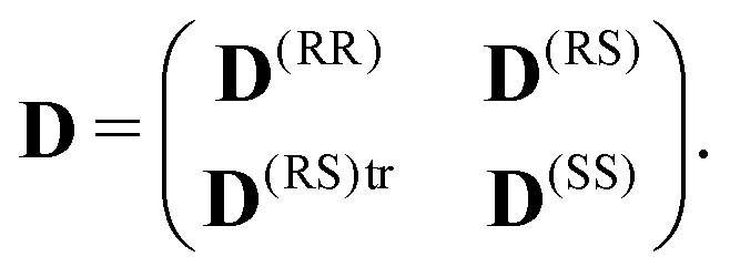
1. elements D(RR)i ≡ D(RR)ii of the diagonal rotational block D(RR) of D
2. first three eigenvalues of the set of eigenvalues obtained by full diagonalization of D and sorted in ascending order.
3. eigenvalues of the rotational diffusion tensor for the rigid molecule obtained with the DiTe2 software package,32 using the same hydrodynamic model and the same conditions described above.
A strikingly good agreement is found between the eigenvalues of the rotational diffusion tensor of the rigid molecule (set 3) and the lowest three eigenvalues of the (fully diagonalized) D matrix (set 2). Therefore, upon coordinate transformation the diagonalization of D seems to lead to a separation of motions, with the three separated eigenvalues being close to the rotational diffusion of the molecule as if it was rigid. The two sets of eigenvalues show an overall decreasing trend with increasing systems size and complexity. In contrast, the three elements of the diagonal rotational block of D(RR) (set 1) do not exhibit a clear trend with increasing system size, and except for the first (and smallest) system their values are one or two orders of magnitude smaller than the respective values from the other two sets. This is in line with the fact that the elements of D(RR)i relate to the rotation of a small subsystem made of the triplet of atoms used to define the molecular frame.
3.3 Analysis of the roto-conformational diffusion tensor
Interesting information can be gained through the analysis of the remaining blocks of the roto-conformational diffusion tensor D. In fact, the diagonalization of the conformational block of the diffusion tensor leads to the definition of a set of ‘normal modes’, each defined by an eigenvector (a column of the T matrix) and associated to a given eigenvalue D(SS)i ≡ D(SS)ii which has units of a frequency. These normal modes are linear combinations of the original set of internal coordinates q with coefficients being the elements of the respective eigenvector. Their character, in terms of their motion, can be thus inferred by the analysis of these coefficients. In particular, the contribution to a given j-th normal mode coming from the motion associated with a given internal coordinate qi can be estimated as the square of the matrix element Tij, with the squares of the element of each j-th column of T summing up to one.On the other hand, the analysis of the elements of the roto-conformational block D(SR) provides information on the coupling between the internal degrees of freedom and the external rotation.
 | ||
| Fig. 2 (a) Molecular structure of DMF. (b) Color plot of the elements Tij2 of the matrix diagonalizing the internal block (SS) of the diffusion matrix. Each row is labeled with a string indicating the kind of motion (‘S’ for stretching, ‘B’ for bending, ‘T’ for torsion) and the IDs (see panel a) of the atoms associated with that motion, listed in the same order as they appear in the Z matrix. (c) Elements D(SS)i (in fs−1), i.e. eigenvalues of the internal block (SS) of the diffusion matrix. (d) Extent of the coupling between the internal motions (each described by the i the normal mode) and the overall rotation. | ||
The roto-conformational coupling (panel d) is strong (high values of |D(SR)ij|/|D(SS)i − D(RR)j|) for only a few normal modes with the lowest frequencies (thus mainly represented by torsion motions). In particular, the first two normal modes exhibit by far the highest coupling with external rotation, while the remaining modes turn out to be negligibly coupled to it. The analysis of the squared elements of the first two columns of the T matrix (panel b) reveals that the internal motions mostly coupled with the external rotation are the C2–N3–C–H torsions (see panel a for atom numbering), with the last two atoms being one of the three CH pairs of each methyl group.
A measure of the ‘coldness’/‘hotness’ of the atoms (i.e. the involvement of atoms in motions associated with lower or higher frequencies), can be computed as follows:
 | (7) |
 | ||
| Fig. 3 Atomic average frequencies in DMF computed as per eqn (7) (see text for discussion). | ||
One may further push the analysis to the contribution of each atom in a given type of motion (stretchings, bendings, torsions) for a given frequency range. To this purpose the following expression can be used:
 | (8) |
 | ||
| Fig. 4 Contribution of the atoms of DMF to stretchings, bendings and torsions in three different frequency ranges (see text for discussion). | ||
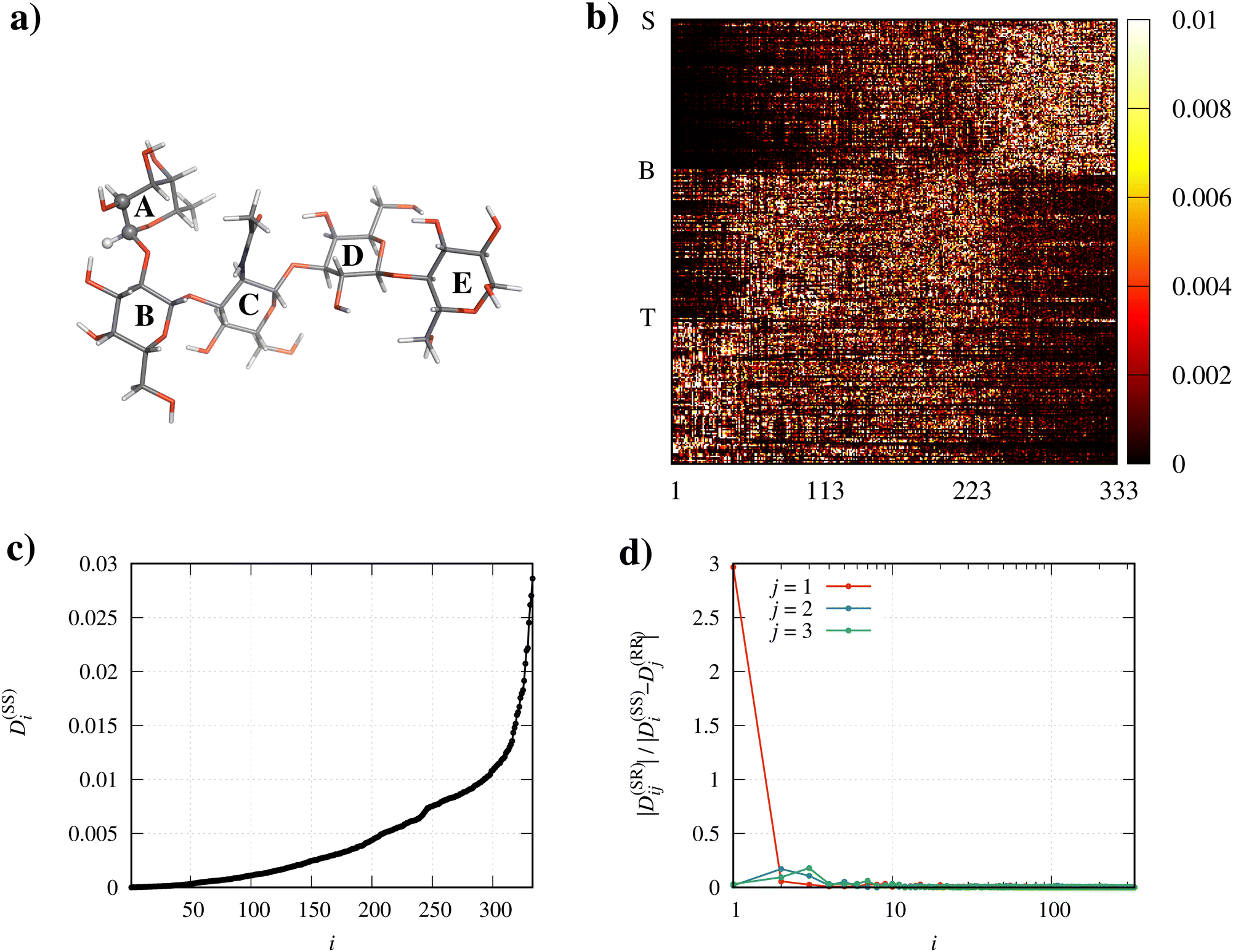 | ||
| Fig. 5 (a) Molecular structure of LNF, with sugar units labeled with letters from A to E. (b) Color plot of the elements Tij2 of the matrix diagonalizing the internal block (SS) of the diffusion matrix. The initial row of the stretchings block (rows 1–112), of the bendings block (rows 113–222), and of the torsions block (rows 223–333) is labeled with ‘S’, ‘B’, and ‘T’, respectively. (c) Elements D(SS)i (in fs−1), i.e. eigenvalues of the internal block (SS) of the diffusion matrix. (d) Extent of the coupling between the internal motions (each described by the i the normal mode) and the overall rotation (note that the abscissa is in logarithmic scale). | ||
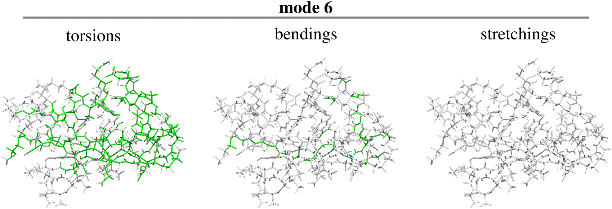
Panel d shows that there is only one normal mode, precisely the lowest-frequency one, which is tightly coupled to the overall rotation of the molecule. The nature of this mode can be appreciated by inspection of Fig. 6, where the atom connections involved in the torsions (left panel), bendings (center panel) and stretchings (right panel) contributing to the mode with value Tij2 above a given threshold are highlighted in green. The threshold is here set to 1/N (with N, as already mentioned, being the number of internal degrees of freedom), i.e. exactly equal to the average value of all contributions to that mode by the original internal coordinates q. In other words, in the panels of Fig. 6, only the connections between atoms involved in motions contributing above average to the mode are highlighted. The figure thus reveals that the only normal mode significantly coupled to the external rotation results mainly from torsions involving the atoms of the polymer backbone, plus one coordinate relating to the bending motion of three of the sugar rings with respect to the remaining two. For LNF we also analyzed how both the parameters relating to physical conditions and the choice of the triplet of atoms defining the orientation frame affect the above discussed results. Results are fully reported and discussed in the ESI.†
 | ||
| Fig. 6 Character of the lowest frequency (and highest coupling with external motion) normal mode in terms of the constituting torsions, bendings and stretchings (see text for discussion) for LNF. | ||
Focusing now on the atom ‘hotness’, Fig. 7 shows the atomic average frequencies of the atoms using the same color scale as in Fig. 3, ranging from white (coldest atom) to red (hottest atom). In this case, the hottest atom is the only terminal oxygen atom, which is bound to a single carbon atom and is thus mainly involved in the stretching of this bond. On the other hand, the coldest atoms are the carbon and oxygen atoms constituting the oligomer backbone linking the sugar rings, which are mainly involved in slow torsion motions.
 | ||
| Fig. 7 Atomic average frequencies in LNF computed as per eqn (7) (see text for discussion). | ||
Also in this case, the matrix of the color plots (Fig. 8) illustrating the contribution of the atoms in different kind of motions for the three above envisaged frequency ranges (identified by index ranges[1,50], [51,240], and [241,333]) reflects the features of the color plot of the T matrix reported in panel b of Fig. 5.
 | ||
| Fig. 8 Contribution of the atoms of LNF to stretchings, bendings and torsions in three different frequency ranges (see text for discussion). | ||
 | ||
| Fig. 9 (a) Molecular structure of GB3. (b) Color plot of the elements Tij2 of the matrix diagonalizing the internal block (SS) of the diffusion matrix. The initial row of the stretchings block (rows 1–861), of the bendings block (rows 862–1720), and of the torsions block (rows 1721–2580) is labeled with ‘S’, ‘B’, and ‘T’, respectively. (c) Elements D(SS)i (in fs−1), i.e. eigenvalues of the internal block (SS) of the diffusion matrix. (d) Extent of the coupling between the internal motions (each described by the i the normal mode) and the overall rotation (note that the abscissa is in logarithmic scale). | ||
 | ||
| Fig. 10 Character of the fifth normal mode in terms of the constituting torsions, bendings and stretchings for GB3 (see text for discussion). | ||
 | ||
| Fig. 11 Character of the sixth normal mode in terms of the constituting torsions, bendings and stretchings for GB3 (see text for discussion). | ||
The two figures show that the modes mainly results from torsions and bendings involving the atoms of the polymer backbone, plus a stretching of the bond linking the S-methyl thioether side chain of the first (methionine) residue to the protein backbone.
The atomic average frequencies for GB3 can be visualized in Fig. 12, where the same color scale is used as in the previously discussed Fig. 3 and 7, i.e. ranging from white (coldest atom) to red (hottest atom). In line with the results on the smaller polymer LNF, the hottest atoms are here the ‘external’ terminal oxygens, while the colder atoms are the more ‘internal’ carbon and nitrogen atoms constituting the polymer backbone. For this last system too, the matrix of the color plots (Fig. 13) illustrating the contribution of the atoms in different kinds of motions for the three above envisaged frequency ranges (identified by index ranges [1,280], [281,1800], and [1801,2580]) reflects the features of the color plot of the T matrix reported in panel b of Fig. 9.
 | ||
| Fig. 12 Atomic average frequencies in GB3 computed as per eqn (7) (see text for discussion). | ||
 | ||
| Fig. 13 Contribution of the atoms of GB3 to stretchings, bendings and torsions in three different frequency ranges (see text for discussion). | ||
4. Conclusions
Based on the previously defined systematic approach to build rigorous stochastic models of flexible molecules in solution from first principles,20,21 we have considered in this paper the diffusive limit obtained upon assumption that momenta relax much faster then positional coordinates. For systems moving in isotropic environments in which the internal energy is independent from the orientation of the molecular frame in the laboratory frame, averaging out all momenta leads, not surprisingly, to a framework in which mechanical coupling disappears, and internal and external degrees freedom are coupled only by friction terms. The resulting FP equation is thus determined by one main tensorial parameter, namely the scaled roto-conformational diffusion tensor, which accounts for the influence of both conservative and dissipative forces and describes the molecular mobility via a precise definition of internal–external and internal–internal couplings.Focusing on a set of molecular systems of increasing complexity ranging from dimethylformamide, to several oligosaccharides and a protein domain, we showed how the rich and informative structure of the scaled roto-conformational diffusion tensor can be analyzed to extract quantitative information on the molecular mobility. In particular, the analysis of the eigenvectors and eigenvalues of the matrix diagonalizing the conformational block of the diffusion tensor provides a quantitative picture of the time scales of the different molecular motions, putting on quantitative grounds, for instance, the time-scale separation between stretching, bending, and torsion motions. Moreover, a suitable combination of the elements of the eigenvector matrix leads to an informative definition of the ‘coldness’/‘hotness’ of the atoms which can be used to quantitatively assess the involvement or contribution of a given atom in specific internal modes. Thus for instance, the intuitive consideration that the coldest atoms of the considered five-units oligosaccharide and protein domain are those constituting the polymer backbone, mainly involved in slow torsion motions, while the hottest atoms are the terminal oxygen atoms mainly involved in stretching motions, could be put on a thorough quantitative ground. Finally, the analysis of the non diagonal block of the scaled roto-conformational diffusion tensor leads to the precise determination of the few internal modes strongly coupled with the overall external rotation. The scaled roto-conformational diffusion tensor can thus be conveniently used as a gauge of molecular flexibility, also with the aim of determining a cut-off in the degrees of freedom to be included in the full solution of the related FP equation. Work is ongoing in our group on the numerical resolution of this equation with a focus on the computation of observables that can be assessed through various spectroscopic techniques including NMR and neutron spectroscopy, which simultaneously accesses spatial and time correlations (as opposed to the angular correlations probed by NMR).
The analysis of molecular flexibility presented in this work can be used as an alternative approach to the selection of essential dynamics in macromolecules, including in the analysis the flexibility in terms of characteristic time scales, instead of just energy arguments. The idea is to be able to extract such an essential dynamics (relevant coordinates) by analyzing short (with respect to the time scales required to interpret slow dynamics) MD trajectories. Machine learning techniques33,34 are expected to be efficiently employed to pursue the best essential dynamics selection with respect to the physical observable that is being interpreted (e.g., NMR relaxation).
Author contributions
Sergio Rampino: formal analysis, investigation, conceptualization, software, validation, visualization, writing (original draft). Mirco Zerbetto: software, validation, conceptualization, resources, writing (review & editing). Antonino Polimeno: conceptualization, methodology, supervision, resources, project administration, writing (review & editing).Conflicts of interest
There are no conflicts to declare.Acknowledgements
Computational work has been carried out on the C3P (Computational Chemistry Community in Padova) HPC facility of the Department of Chemical Sciences of the University of Padova. This work was supported by grants from the University of Padova (P-DISC # Adaptive schemes for complex interactions in molecular dynamics simulations BIRD2020-UNIPD).Notes and references
- T. Mittag, L. E. Kay and J. D. Forman-Kay, J. Mol. Recognit., 2009, 23, 105–116 Search PubMed.
- V. N. Uversky, J. R. Gillespie and A. L. Fink, Proteins, 2000, 41, 415–427 CrossRef CAS.
- D. Korzhnev, M. Billeter, A. Arseniev and V. Orekhov, Prog. Nucl. Magn. Reson. Spectrosc., 2001, 38, 197–266 CrossRef CAS.
- J. Lippincott-Schwartz, E. Snapp and A. Kenworthy, Nat. Rev. Mol. Cell Biol., 2001, 2, 444–456 CrossRef CAS PubMed.
- H. Ihee, M. Wulff, J. Kim and S. Ichi Adachi, Int. Rev. Phys. Chem., 2010, 29, 453–520 Search PubMed.
- T. Ando, N. Kodera, E. Takai, D. Maruyama, K. Saito and A. Toda, Proc. Natl. Acad. Sci. U. S. A., 2001, 98, 12468–12472 CrossRef CAS PubMed.
- M. Grimaldo, F. Roosen-Runge, F. Zhang, F. Schreiber and T. Seydel, Q. Rev. Biophys., 2019, 52, e7 CrossRef.
- J. Wang, S. Olsson, C. Wehmeyer, A. Pérez, N. E. Charron, G. de Fabritiis, F. Noé and C. Clementi, ACS Cent. Sci., 2019, 5, 755–767 CrossRef CAS PubMed.
- P. Gkeka, G. Stoltz, A. Barati Farimani, Z. Belkacemi, M. Ceriotti, J. D. Chodera, A. R. Dinner, A. L. Ferguson, J.-B. Maillet, H. Minoux, C. Peter, F. Pietrucci, A. Silveira, A. Tkatchenko, Z. Trstanova, R. Wiewiora and T. Lelièvre, J. Chem. Theory Comput., 2020, 16, 4757–4775 CrossRef CAS PubMed.
- M. M. Triton, Phys. Rev. Lett., 1996, 77, 1905–1908 CrossRef PubMed.
- D. Ben-Avraham, Phys. Rev. B: Condens. Matter Mater. Phys., 1993, 47, 14559–14560 CrossRef CAS PubMed.
- A. R. Atilgan, S. R. Durell, R. L. Jernigan, M. C. Demirel, O. Keskin and I. Bahar, Biophys. J., 2001, 80, 505–515 CrossRef CAS PubMed.
- E. Eyal, L.-W. Yang and I. Bahar, Bioinformatics, 2006, 22, 2619–2627 CrossRef CAS PubMed.
- N. Go, T. Noguti and T. Nishikawa, Proc. Natl. Acad. Sci. U. S. A., 1983, 80, 3696–3700 CrossRef CAS PubMed.
- B. Brooks and M. Karlplus, Proc. Natl. Acad. Sci. U. S. A., 1983, 80, 6571–6575 CrossRef CAS PubMed.
- P. Dauber-Osguthorpe and D. J. Osguthorpe, J. Am. Chem. Soc., 1989, 112, 7921–7935 CrossRef.
- P. Dauber-Osguthorpe and D. J. Osguthorpe, Biochemistry, 1990, 29, 8223–8228 CrossRef CAS PubMed.
- I. Bahar, B. Erman, T. Haliloglu and R. L. Jernigan, Biochemistry, 1997, 36, 13512–13523 CrossRef CAS PubMed.
- A. Amedei, A. B. M. Linssen and H. J. C. Berendsen, Proteins, 1993, 17, 412–425 CrossRef PubMed.
- A. Polimeno, M. Zerbetto and D. Abergel, J. Chem. Phys., 2019, 150, 184107 CrossRef PubMed.
- A. Polimeno, M. Zerbetto and D. Abergel, J. Chem. Phys., 2019, 150, 184108 CrossRef PubMed.
- H. Goldstein, Classical Mechanics, Addison-Wesley, 1980 Search PubMed.
- R. Zwanzig, Physica, 1964, 30, 1109–1123 CrossRef.
- R. Zwanzig, J. Stat. Phys., 1973, 9, 215–220 CrossRef.
- B. Yoon, J. Deutch and J. Freed, J. Chem. Phys., 1975, 62, 4687 CrossRef CAS.
- R. Pendrill, O. Engström, A. Volpato, M. Zerbetto, A. Polimeno and G. Widmalm, Phys. Chem. Chem. Phys., 2016, 18, 3086–3096 RSC.
- M. Zerbetto, A. Polimeno, D. Kotsyubynskyy, L. Ghalebani, J. Kowalewski, E. Meirovitch, U. Olsson and G. Widmalm, J. Chem. Phys., 2009, 131, 234501 CrossRef PubMed.
- M. Zerbetto, T. Angles d'Ortoli, A. Polimeno and G. Widmalm, J. Phys. Chem. B, 2018, 122, 2287–2294 CrossRef CAS PubMed.
- D. Kotsyubynskyy, M. Zerbetto, M. Soltesova, O. Engström, R. Pendrill, J. Kowalewski, G. Widmalm and A. Polimeno, J. Phys. Chem. B, 2012, 116, 14541–14555 CrossRef CAS PubMed.
- M. Zerbetto, D. Kotsyubynskyy, J. Kowalewski, G. Widmalm and A. Polimeno, J. Phys. Chem. B, 2012, 116, 13159–13171 CrossRef CAS PubMed.
- S. Rampino, M. Zerbetto and A. Polimeno, Molecules, 2021, 26, 2418 CrossRef CAS PubMed.
- J. Campeggio, A. Polimeno and M. Zerbetto, J. Comput. Chem., 2019, 40, 697–705 CAS.
- R. R. Coifman, I. G. Kevrekidis, S. Lafon, M. Maggioni and B. Nadler, Multiscale Model. Simul., 2008, 7, 842–864 CrossRef.
- W. Chen, A. R. Tan and A. L. Ferguson, J. Chem. Phys., 2018, 149, 072312 CrossRef PubMed.
Footnote |
| † Electronic supplementary information (ESI) available: Results on the roto-conformational diffusion tensor (analogues of Fig. 2, 5 and 9) for the remaining five oligosaccharides, brief review of the Fokker–Planck equation in internal coordinates, and derivation of the Smoluchowski equation by projetion of the momenta. See DOI: https://doi.org/10.1039/d3cp01382k |
| This journal is © the Owner Societies 2023 |