
 Open Access Article
 This Open Access Article is licensed under a
 Creative Commons Attribution 3.0 Unported Licence
Metallocene-coupled cumulenes: a quest for chiral single-molecule magnets†‡
Soumik
Das
a,
Anirban
Misra
*a and
Suranjan
Shil
 *b
*b
aDepartment of Chemistry, University of North Bengal, Raja Rammohunpur, Siliguri 734013, West Bengal, India. E-mail: anirbanmisra@nbu.ac.in
bManipal Centre for Natural Sciences (Centre of Excellence), Manipal Academy of Higher Education, Planetorium Complex, Madhavnagar, Manipal 576104, Karnataka, India. E-mail: suranjan.shil@manipal.edu; Tel: +91-9434801574
First published on 3rd April 2023
Abstract
In this work, we computationally investigated nickelocene and chromocene–coupled linear carbon chains. The designed systems are [Ni]–Cn–Ni], [Cr]–Cn–[Cr] and [Cr]–Cn–[Ni] (n = 3 to 9), where [Ni], [Cr] and Cn represent nickelocene (NiCp2, Cp = cyclopentadienyl), chromocene (CrCp2) and linear carbon chains respectively. The magnetic properties of these systems were computationally investigated by a density functional theory–based method. Ferromagnetic ground states were observed for [Ni]–Cn–[Ni] and [Cr]–Cn–[Cr] complexes for couplers with odd numbers of carbon atoms (n = 3, 5, 7 and 9), whereas antiferromagnetic ground states result for couplers with even numbers of carbon atoms (n = 4, 6 and 8). However, a totally opposite trend is followed by [Cr]–Cn–[Ni] complexes due to the spin polarization inside the chromocene. The calculation and study of magnetic anisotropy for all the ferromagnetic complexes suggest that the [Ni]–Cn–[Ni] complexes with coupler of odd number of carbon atoms will be suitable for the synthesis of single-molecule magnets among the designed complexes.
Introduction
A single-molecule magnet (SMM) is an organic or metal–organic complex with molecular level magnetic properties. In contrast to bulk magnets, single-molecule magnets exhibit magnetic hysteresis of purely molecular origin in a certain temperature range. The design and characterization of SMMs have attracted tremendous attention from both experimental and theoretical scientists1–12 because of potential applications of such materials in high-density information storage, quantum computing, magnetic refrigeration and in biomedical field such as MRI.13–17 A Mn12Ac complex18 was discovered in 1991 and extensively investigated as a SMM. Ishikawa et al. reported first double-decker lanthanide single-ion magnets.19 Dysprosium-based single-molecule magnets were studied by several researchers.20,21 Kotrle et al. computationally investigated dysprosium double-decker complexes, [Dy(L)2]+/3+, with inorganic aromatic ring systems (L = P5−, N5−, B3N3H6, B3P3H6, and B3S3H3).22 Spin sources of organic origin like organic radicals were also investigated as potential candidates for designing single-molecule magnets.23 Organic radicals were connected by conjugated couplers, and the dependency of the magnetic interaction between radical centres on length, planarity, dihedral angle, etc., of the couplers was computationally investigated by several researchers. Ali et al. found that with the increase in conjugated coupler length, the strength of magnetic interaction between nitronyl nitroxide radical centers decreased.24 The dihedral angle between two radical centers connected through couplers has profound effects on magnetic interaction. With the increase in dihedral angle between two spin centers, the coupling constant value and magnetic interaction decrease.25,26Linear carbon chains such as allenes and cumulenes have interesting electronic structures associated with fascinating properties, which attracted the attention of the scientific community.27–29 Allenes and cumulenes with odd numbers of carbon atoms are chiral in nature because of the presence of a chiral axis, whereas cumulenes with even numbers of carbon atoms are achiral. The presence of chirality in the linear carbon chain with odd numbers of carbon atoms inspired scientists to design chiral magnets. Sarbadhikary et al. have designed and investigated chiral organic magnetic molecules with allenes and cumulenes as couplers.30 They have found that with the increase in carbon chain length, the spin-density on the coupler increases, the HOMO–LUMO energy gap decreases and, hence, the magnetic exchange coupling constant increases. This is clearly opposite to the trend observed for conjugated organic systems as couplers. Shil et al. have designed cobaltocene-coupled cumulenes and investigated their magnetic and transport properties.31
In this work, we chose nickelocene and chromocene as spin sources. Both NiCp2 and CrCp2 have triplet ground state. The qualitative d orbital splitting of the metals and occupations are given in Fig. 1. We have designed three types of magnetic systems ([Ni]–Cn–[Ni], [Cr]–Cn–[Cr] and [Cr]–Cn–[Ni], here n = 3 to 9), shown in Fig. 2. The impact of different factors such as geometry, HOMO–LUMO (here SOMO4 (α)–LUMO (α)) energy gap and spin-density on magnetic property were investigated using density functional theory (DFT). We found that [Ni]–Cn–[Ni] and [Cr]–Cn–[Cr] show ferromagnetic interactions for couplers with odd numbers of carbon atoms and antiferromagnetic interactions for couplers with even numbers of carbon atoms, whereas for [Cr]–Cn–[Ni], the reverse trend is observed.
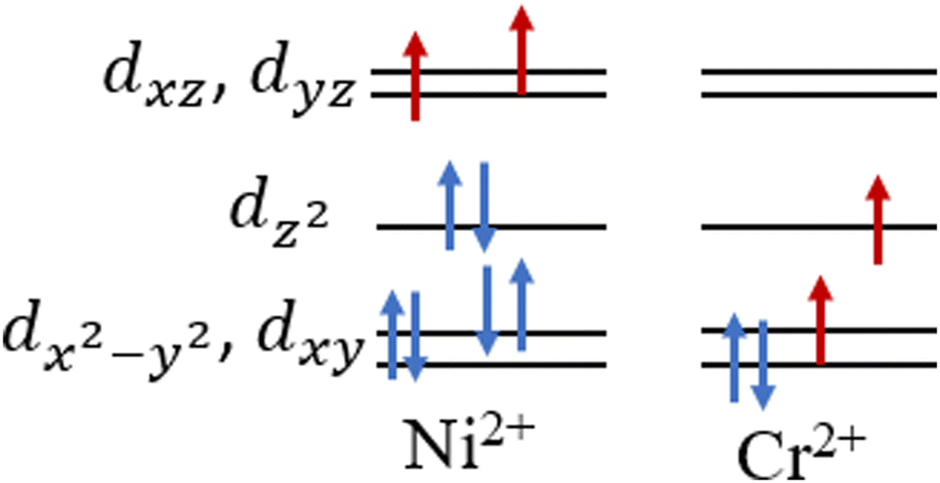 | ||
| Fig. 1 Electronic configurations and splitting of metal d orbitals in nickelocene and chromocene in their ground state. | ||
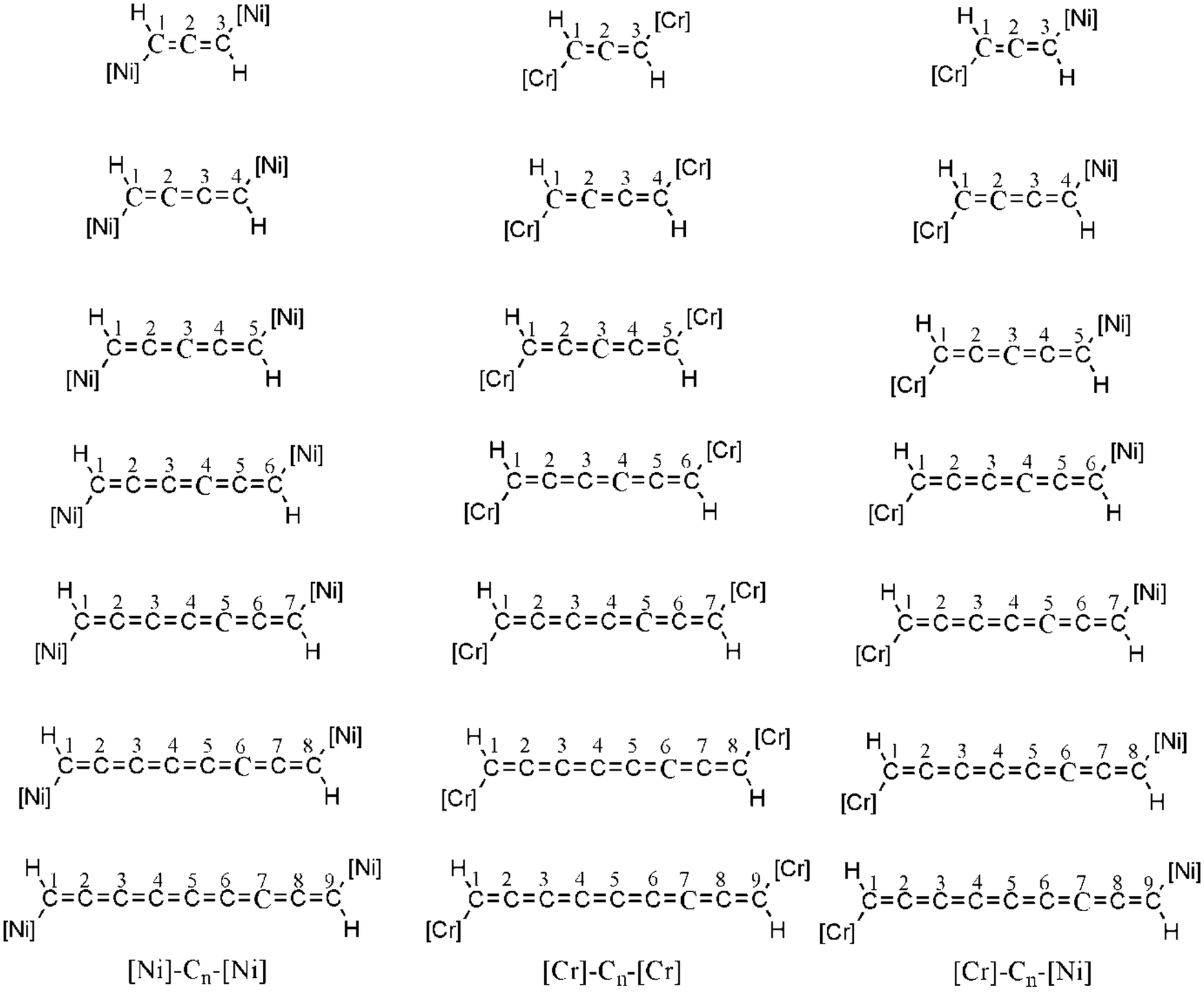 | ||
| Fig. 2 Designed [Ni]–Cn–[Ni], [Cr]–Cn–[Cr] and [Cr]–Cn–[Ni] systems, here n = 3 to 9. [Ni] and [Cr] represent nickelocene and chromocene respectively. | ||
Theoretical and computational methods
The magnetic interaction between two magnetic sites 1 and 2 can be expressed by the Heisenberg spin Hamiltonian as follows:| H = −2JŜ1·Ŝ2 | (1) |
Though pure spin states of a system can be described reliably by multiconfigurational approaches, they are computationally expensive in nature. Hence, we used a DFT-based cost-effective broken-symmetry approach given by Noodleman, which was found to describe magnetism in a reliable way.32,33 Among different available equations for the determination of the magnetic exchange coupling constant, we used the spin-projected formula given by Yamaguchi.34–37 This formula is applicable for a wide range of orbital overlap and appears as follows:
 | (2) |
 | ||
| Fig. 3 Spin–flip strategy used in this computational study for the generation of broken-symmetry solutions. | ||
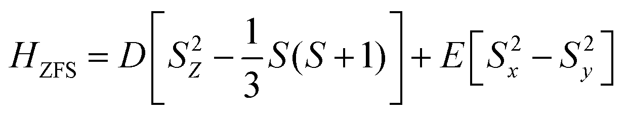
Magnetic anisotropy is one of the very important aspects for the suitable design of single-molecule magnets.38–40 The relations between the axial ZFS parameter D, the rhombic ZFS parameters E and the anisotropy tensor components (γxx, γyy, γzz) can be written as follows:
 | (3) |
All the calculations were done using unrestricted density functional theory (DFT). Two functionals (B3LYP and MN12SX) were used along with the 6-311++g(d,p) basis set, so that the results can be compared and validated. The viability of the optimized structures was confirmed from the wavefunction stability check and absence of any imaginary frequency. All the calculations were performed using the Gaussian 16W software.42 The zero-field splitting (D) parameter was calculated using the ORCA43 software.
Results and discussion
Magnetic exchange coupling constant
It is very important to understand the contribution of different factors such as geometry and spin-density distribution to the magnetic property of a system before synthesizing a suitable magnetic molecule. We calculated the intramolecular magnetic exchange coupling constant with two different functionals (B3LYP and MN12SX) using the same basis set, 6-311++g(d,p) to check the reliability and variation of the results. Both the functionals are known to produce reliable results on the magnetic property.44 Puhl et al. synthesized dicobaltocene complexes and evaluated the exchange coupling constant experimentally and computationally.45 There results indicated that the DFT-based methods are well verged with the experimental findings. The calculated values of the magnetic exchange coupling constant for the three types of systems ([Ni]–Cn–[Ni], [Cr]–Cn–[Cr] and [Cr]–Cn–[Ni]) are shown in a tabular form (Table 1). From Table 1, it is clear that both the functionals (B3LYP and MN12SX) produce consistent values of coupling constant. Four important observations can be drawn after analysing the coupling constant values (Table 1).| System | B3LYP | MN12SX | ||||
|---|---|---|---|---|---|---|
| [Ni]–Cn–[Ni] | [Cr]–Cn–[Cr] | [Cr]–Cn–[Ni] | [Ni]–Cn–[Ni] | [Cr]–Cn–[Cr] | [Cr]–Cn–[Ni] | |
| C3 | 4.55 | 0.35 | −0.27 | 3.40 | 0.11 | −0.11 |
| C5 | 12.64 | 3.29 | −6.36 | 11.94 | 1.92 | −4.45 |
| C7 | 27.55 | 13.13 | −19.09 | 23.83 | 6.50 | −11.53 |
| C9 | 53.20 | 37.46 | −44.50 | 41.17 | 14.52 | −23.26 |
| C4 | −108.49 | −11.07 | 90.15 | −90.14 | −8.01 | 33.12 |
| C6 | −148.43 | −45.43 | 204.60 | −116.37 | −18.78 | 81.62 |
| C8 | −194.05 | −112.25 | 380.20 | −148.18 | −44.62 | 148.64 |
(i) With the increase in sp carbon chain length (for even and odd number of chains), magnetic exchange coupling constant values increase for all three types of systems.
(ii) [Ni]–Cn–[Ni] and [Cr]–Cn–[Cr] complexes show ferromagnetic ground states for couplers with odd numbers of sp carbons and antiferromagnetic ground states for couplers with even numbers of sp carbon atoms, whereas [Cr]–Cn–[Ni] systems show ferromagnetic ground states for even numbers of sp carbon chain and antiferromagnetic ground states for odd numbers of sp carbon chain. These results of [Cr]–Cn–[Ni] complexes are clearly opposite to the results for [Ni]–Cn–[Ni] and [Cr]–Cn–[Cr] systems. It demands careful inspection of spin-density distributions of the designed systems, as spin-density distribution provides information about the mechanism and type of interaction between spin centers.
(iii) For [Ni]–Cn–[Ni] and [Cr]–Cn–[Cr] complexes, the absolute values of coupling constants for antiferromagnetic systems are higher than that of the ferromagnetic systems. However, for [Cr]–Cn–[Ni], the opposite trend is observed.
(iv) The coupling constant values for [Ni]–Cn–[Ni] complexes are greater than the corresponding J values for [Cr]–Cn–[Cr] systems in spite of having the same number of unpaired electrons in their ground states.
The observations found from Table 1 prompt us to examine different parameters of optimized geometry, spin-density distribution and frontier molecular orbital energies (SOMO4 (α)–LUMO (α) energy gap).
Molecular structure
Molecular geometry is an important factor as almost all properties including reactivity, stability, spin-density distribution, and magnetic property of any system depend on the geometry. The bond lengths of the coupler of all the optimized systems are given in Tables 2, 3 and 4. Bond angles are summarised in Tables S1, S2 and S3 (ESI‡).| System | C1–C2 | C2–C3 | C3–C4 | C4–C5 | C5–C6 | C6–C7 | C7–C8 | C8–C9 | Average bond length | C–L | C–R |
|---|---|---|---|---|---|---|---|---|---|---|---|
| C3 | 1.312 | 1.312 | 1.312 | 1.464 | 1.464 | ||||||
| C5 | 1.325 | 1.274 | 1.274 | 1.325 | 1.300 | 1.451 | 1.451 | ||||
| C7 | 1.332 | 1.267 | 1.283 | 1.283 | 1.267 | 1.332 | 1.294 | 1.443 | 1.443 | ||
| C9 | 1.337 | 1.263 | 1.289 | 1.276 | 1.276 | 1.289 | 1.263 | 1.337 | 1.291 | 1.438 | 1.438 |
| C4 | 1.334 | 1.256 | 1.334 | 1.308 | 1.447 | 1.447 | |||||
| C6 | 1.335 | 1.258 | 1.299 | 1.258 | 1.335 | 1.297 | 1.444 | 1.444 | |||
| C8 | 1.336 | 1.259 | 1.296 | 1.262 | 1.296 | 1.259 | 1.336 | 1.292 | 1.441 | 1.441 |
| System | C1–C2 | C2–C3 | C3–C4 | C4–C5 | C5–C6 | C6–C7 | C7–C8 | C8–C9 | Average bond length | C–L | C–R |
|---|---|---|---|---|---|---|---|---|---|---|---|
| C3 | 1.311 | 1.311 | 1.311 | 1.467 | 1.467 | ||||||
| C5 | 1.323 | 1.274 | 1.274 | 1.323 | 1.299 | 1.456 | 1.456 | ||||
| C7 | 1.330 | 1.268 | 1.283 | 1.283 | 1.268 | 1.330 | 1.294 | 1.449 | 1.449 | ||
| C9 | 1.336 | 1.263 | 1.289 | 1.276 | 1.276 | 1.289 | 1.263 | 1.336 | 1.291 | 1.444 | 1.444 |
| C4 | 1.333 | 1.256 | 1.333 | 1.307 | 1.451 | 1.451 | |||||
| C6 | 1.335 | 1.258 | 1.300 | 1.258 | 1.335 | 1.297 | 1.449 | 1.449 | |||
| C8 | 1.347 | 1.252 | 1.306 | 1.256 | 1.306 | 1.252 | 1.347 | 1.295 | 1.445 | 1.445 |
| System | C1–C2 | C2–C3 | C3–C4 | C4–C5 | C5–C6 | C6–C7 | C7–C8 | C8–C9 | Average bond length | C–L | C–R |
|---|---|---|---|---|---|---|---|---|---|---|---|
| C3 | 1.311 | 1.311 | 1.311 | 1.468 | 1.463 | ||||||
| C5 | 1.323 | 1.274 | 1.273 | 1.324 | 1.299 | 1.456 | 1.451 | ||||
| C7 | 1.330 | 1.268 | 1.282 | 1.283 | 1.267 | 1.330 | 1.293 | 1.450 | 1.445 | ||
| C9 | 1.334 | 1.264 | 1.288 | 1.277 | 1.276 | 1.288 | 1.264 | 1.334 | 1.290 | 1.445 | 1.441 |
| C4 | 1.339 | 1.252 | 1.340 | 1.310 | 1.444 | 1.439 | |||||
| C6 | 1.348 | 1.250 | 1.312 | 1.250 | 1.349 | 1.302 | 1.435 | 1.429 | |||
| C8 | 1.357 | 1.245 | 1.317 | 1.247 | 1.317 | 1.245 | 1.357 | 1.298 | 1.427 | 1.420 |
From Tables 2, 3 and 4, it is clear that individual bond lengths for all three types of systems vary from 1.24 Å to 1.31 Å, which is in between the C–C double bond (1.34 Å) and triple bond lengths (1.20 Å). The average bond distances for all the systems vary from 1.28 Å to 1.31 Å. These findings clearly indicate the allene-like electronic structure of the coupler for all the systems (both for even and odd numbers of carbon atom couplers). Another important observation is the decrease in the average bond length with the increase in the number of carbon atoms in the Cn chain (n = 3, 5, 7, and 9 and n = 4, 6, and 8) for all the designed systems. The C–L and C–R bond lengths also decrease with the increase in the number of carbon atoms. All the bond angles (Tables S1, S2 and S3, ESI‡) are nearly 180°, which is the signature property of the sp carbon atom. Similar results are obtained with the MN12SX functional (Tables S4, S5, S6, S7, S8 and S9, ESI‡). Hence, it can be concluded from the analysis of bond lengths and bond angles that the couplers (Cn chain) behave like allene and cumulene chains.
Spin-density analysis
Magnetic interaction between two magnetic sites largely depends upon the spin-density distribution. The analysis of spin-density distribution can provide important insights into the mechanism of interaction between two spin centers. The magnetic exchange coupling constant value depends on the distribution of π electron density between two magnetic sites. Greater distribution of electron density between magnetic centers indicates stronger interaction, resulting in a larger coupling constant value. Spin-density alternation rule is an effective tool for predicting the nature of magnetic interaction between two magnetic sites.30,46,47 When two spin centers are connected with even number of conjugated bonds, ferromagnetic interaction takes place, whereas antiferromagnetic interaction takes place if they are connected by odd number of conjugated bonds. According to the spin-density alternation rule, spin centers connected with Cn chains with odd numbers of carbon atoms (n = 3, 5, 7 and 9) would result in ferromagnetic interaction and one should expect antiferromagnetic interaction in case of Cn chains with even numbers of carbon atoms (n = 4, 6 and 8). From Table 1, we can see that [Ni]–Cn–[Ni] and [Cr]–Cn–[Cr] follow the spin-density alternation rulepredicted trend but the opposite tendency is observed for [Cr]–Cn–[Ni]. That is, metallocenes coupled with the Cn chains with n = 3, 5, 7 and 9 produces antiferromagnetic interaction, whereas n = 4, 6 and 8 show ferromagnetic interaction.From Tables 5, 6, 7 and Fig. 4, it is clearly observed that with the increase in Cn chain length (n = 3, 5, 7, and 9 and n = 4, 6, and 8), the average spin-density on each atom of the coupler increases for all the designed complexes. This trend is also observed by Hermann et al. for even cumulene systems.48,49 Sarbadhikary et al. have shown that for allene and cumulene couplers with even and odd numbers of sp carbon atoms, the spin-density on each atom increases with the increase in length, whereas, for conjugated couplers, it decreases.30,49 A linear Cn coupler contains two sp2 hybridized end carbon atoms with one π electron, but the middle carbon atoms are sp hybridized with two π electrons. The sp hybridized middle carbons have greater electronegativity and higher s character. These will lead to greater localization of spin on each atoms of the coupler. Conjugated couplers have only one π electron on each sp2 hybridized carbon atom with less s character and electronegativity. The combined effect of these above-mentioned factors will result in an increase in the spin-density on each atom for a linear Cn chain coupler. As the number of sp hybridized carbon atom increases with the increase in Cn chain length (n = 3, 5, 7, and 9 and n = 4, 6, and 8), the spin-density on the coupler also increases, resulting in a higher coupling constant value. These points clarify our first observation mentioned before.
| System | Ni1 | Ni2 | C1 | C2 | C3 | C4 | C5 | C6 | C7 | C8 | C9 | Average spin-density on each atom of coupler |
|---|---|---|---|---|---|---|---|---|---|---|---|---|
| C3 | 1.167 | 1.167 | −0.054 | 0.128 | −0.054 | 0.079 | ||||||
| C5 | 1.158 | 1.158 | −0.076 | 0.168 | −0.107 | 0.169 | −0.077 | 0.119 | ||||
| C7 | 1.151 | 1.151 | −0.131 | 0.221 | −0.139 | 0.211 | −0.139 | 0.221 | −0.131 | 0.170 | ||
| C9 | 1.141 | 1.141 | −0.171 | 0.261 | −0.203 | 0.285 | −0.170 | 0.284 | −0.203 | 0.261 | −0.172 | 0.223 |
| C4 | −1.147 | 1.147 | 0.181 | −0.146 | 0.146 | −0.181 | 0.164 | |||||
| C6 | −1.139 | 1.139 | 0.216 | −0.163 | 0.211 | −0.211 | 0.163 | −0.216 | 0.197 | |||
| C8 | −1.133 | 1.133 | 0.247 | −0.188 | 0.226 | −0.186 | 0.186 | −0.226 | 0.188 | −0.247 | 0.212 |
| System | Cr1 | Cr2 | C1 | C2 | C3 | C4 | C5 | C6 | C7 | C8 | C9 | Average spin-density on each atom of coupler |
|---|---|---|---|---|---|---|---|---|---|---|---|---|
| C3 | 2.135 | 2.135 | 0.034 | −0.028 | 0.034 | 0.032 | ||||||
| C5 | 2.220 | 2.221 | 0.047 | −0.066 | 0.055 | −0.064 | 0.047 | 0.056 | ||||
| C7 | 2.290 | 2.289 | 0.100 | −0.142 | 0.097 | −0.146 | 0.096 | −0.143 | 0.099 | 0.118 | ||
| C9 | 2.382 | 2.382 | 0.141 | −0.209 | 0.174 | −0.254 | 0.148 | −0.254 | 0.172 | −0.209 | 0.141 | 0.173 |
| C4 | 2.213 | −2.213 | 0.087 | −0.041 | 0.043 | −0.086 | 0.064 | |||||
| C6 | 2.331 | −2.330 | 0.164 | −0.105 | 0.159 | −0.160 | 0.105 | −0.165 | 0.143 | |||
| C8 | 2.343 | −2.341 | 0.240 | −0.151 | 0.189 | −0.176 | 0.176 | −0.189 | 0.149 | −0.240 | 0.189 |
| System | Cr1 | Ni2 | C1 | C2 | C3 | C4 | C5 | C6 | C7 | C8 | C9 | Average spin-density on each atom of coupler |
|---|---|---|---|---|---|---|---|---|---|---|---|---|
| C3 | 2.159 | −1.172 | 0.036 | −0.045 | 0.052 | 0.044 | ||||||
| C5 | −2.221 | 1.161 | −0.054 | 0.108 | −0.082 | 0.126 | −0.072 | 0.088 | ||||
| C7 | −2.298 | 1.152 | −0.103 | 0.170 | −0.112 | 0.177 | −0.122 | 0.192 | −0.125 | 0.143 | ||
| C9 | 2.390 | −1.144 | 0.138 | −0.210 | 0.173 | −0.258 | 0.154 | −0.264 | 0.192 | −0.245 | 0.163 | 0.200 |
| C4 | 2.320 | 1.141 | 0.184 | −0.122 | 0.150 | −0.185 | 0.160 | |||||
| C6 | 2.505 | 1.120 | 0.232 | −0.153 | 0.227 | −0.249 | 0.196 | −0.271 | 0.221 | |||
| C8 | 2.683 | 1.100 | 0.250 | −0.165 | 0.223 | −0.201 | 0.190 | −0.273 | 0.217 | −0.332 | 0.231 |
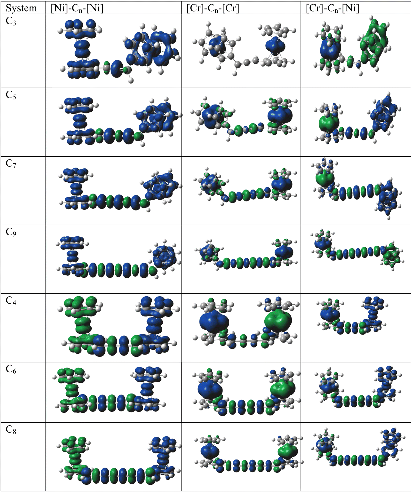 | ||
| Fig. 4 Spin-density distribution plot of high-spin states (quintet) for ferromagnetic and broken-symmetry states (open-shell singlet) for antiferromagnetic complexes calculated in the UB3LYP/6-311++g(d,p) level of theory. Blue and green surfaces represent different phases of spin density. | ||
In [Ni]–Cn–[Ni] and [Cr]–Cn–[Cr] complexes, the same spin is localized on metal atoms for couplers (linear Cn chain) with odd numbers of carbon atoms. However, opposite spin is localized when n is even (Fig. 4). Thus, both [Ni]–Cn–[Ni] and [Cr]–Cn–[Cr] complexes will show ferromagnetic ground state for n = odd and antiferromagnetic ground state for n = even. From Fig. 4, we can see that the same spin is delocalized over the two cyclopentadienyl anion moiety in case of the nickelocene unit. However, in case of chromocene, alpha spin on chromium atom induces beta spin on the two cyclopentadienyl anions and vice versa. That is, spin polarization which is absent in the nickelocene unit is present inside of the chromocene moiety. The mechanism of spin polarization is pictorially depicted in Fig. 5. This difference of spin polarization between chromocene and nickelocene results in the accumulation of the same spin on Cr and Ni atoms in [Cr]–Cn–[Ni] complexes when n is even, whereas the accumulation of opposite spins is observed when n is odd. This mechanism of spin polarization justifies our second observation (Fig. 5). Because of the difference of spin polarization between chromocene and nickelocene moieties, [Cr]–Cn–[Ni] complexes exhibit ferromagnetic ground states when n = even and antiferromagnetic ground states when n = odd.
 | ||
| Fig. 5 Mechanism of spin polarization in [Ni]–Cn–[Ni], [Cr]–Cn–[Cr] and [Cr]–Cn–[Ni]. Mechanism is shown only for n = 3 and 4. | ||
From Tables 5, 6 and 7 (and qualitatively from Fig. 4), we found that the average spin-density on each atom of the coupler is higher for [Ni]–Cn–[Ni], [Cr]–Cn–[Cr] and [Cr]–Cn–[Ni] complexes when n is even. When spin centers are connected with the linear Cn chain with an even number of carbon atoms, they are in the same plane and it results in higher delocalization of π electron density and, hence, higher average spin-density. Higher spin-density indicates stronger magnetic interaction between spin centers. Thus, the value of the coupling constant will be greater when n = even than when n = odd irrespective of the nature of magnetic interaction (ferromagnetic or antiferromagnetic).
Another interesting observation is that, with the increase in coupler length, the spin-density on Cr atom increases (for both n = even and odd), but the spin-density on the Ni atom decreases. That is, the Cr atom has a tendency to localize spin-density on it. As a result, the delocalization of spin-density in [Cr]–Cn–[Cr] complexes is lesser than that of the corresponding [Ni]–Cn–[Ni] systems. This clearly explains the lesser J values for [Cr]–Cn–[Cr] systems than for the corresponding [Ni]–Cn–[Ni] systems.
The above-mentioned conclusions can also be arrived from the analysis of the spin-density distributions obtained from UMN12SX/6-311++g(d,p) as well (Tables S10, S11 and S12, ESI‡).
Molecular orbitals
The energy of the frontier molecular orbitals have profound effects on the magnetic property of a system.26 With the increase in coupler length, the SOMO4 (α)–LUMO (α) gap of the diradicals decreases gradually for couplers with even and odd numbers of carbon atoms (Table 8). However, the magnetic exchange coupling constant increases with the increase in the coupler length. Therefore, the magnetic exchange coupling constant is inversely related to the SOMO4 (α)–LUMO (α) energy gap of the complexes. Therefore, there is a role of LUMO in the magnetic exchange coupling. Not only SOMO4 (α)–LUMO (α) energy gap, but also the occupation number of LUMO is important for stronger magnetic interaction between two spin centers.26 To confirm the effect of LUMO, we have computed the natural orbital occupation of LUMO. From Tables 8 and 9, it is clear that with the decrease in SOMO4 (α)–LUMO (α) energy gap, the occupation number of LUMO increases resulting in a stronger magnetic exchange coupling constant. Not only the energy of orbitals and occupation but also the position of orbitals is important to explain the magnetic interaction in molecular systems. If we look at Fig. 6 and Fig. S1, S2 in the ESI,‡ we can see that the LUMO always resides in between magnetic orbitals. Hence, we may conclude that the magnetic interaction occurs between SOMOs via LUMO. Similar trends of SOMO4 (α)–LUMO (α) energy gaps are found in the UB3LYP/6-31g(d,p) level of theory (Table S15, ESI‡).| System | B3LYP | MN12SX | ||||
|---|---|---|---|---|---|---|
| [Ni]–Cn–[Ni] | [Cr]–Cn–[Cr] | [Cr]–Cn–[Ni] | [Ni]–Cn–[Ni] | [Cr]–Cn–[Cr] | [Cr]–Cn–[Ni] | |
| C3 | 4.44 | 4.41 | 4.27 | 2.23 | 2.89 | 2.18 |
| C5 | 3.45 | 3.82 | 3.41 | 2.20 | 2.82 | 2.09 |
| C7 | 2.88 | 3.30 | 2.80 | 2.12 | 2.70 | 2.07 |
| C9 | 2.51 | 2.88 | 2.39 | 2.00 | 2.51 | 1.92 |
| C4 | 2.77 | 3.20 | 2.96 | 1.82 | 2.59 | 2.04 |
| C6 | 2.26 | 2.69 | 2.51 | 1.77 | 2.33 | 1.86 |
| C8 | 1.93 | 2.38 | 2.24 | 1.49 | 2.03 | 1.72 |
| System | [Ni]–Cn–[Ni] | [Cr]–Cn–[Cr] | [Cr]–Cn–[Ni] |
|---|---|---|---|
| C3 | 0.002 | 0.009 | 0.009 |
| C5 | 0.005 | 0.019 | 0.019 |
| C7 | 0.015 | 0.042 | 0.049 |
| C9 | 0.036 | 0.080 | 0.096 |
| C4 | 0.017 | 0.039 | 0.060 |
| C6 | 0.041 | 0.098 | 0.149 |
| C8 | 0.071 | 0.194 | 0.246 |
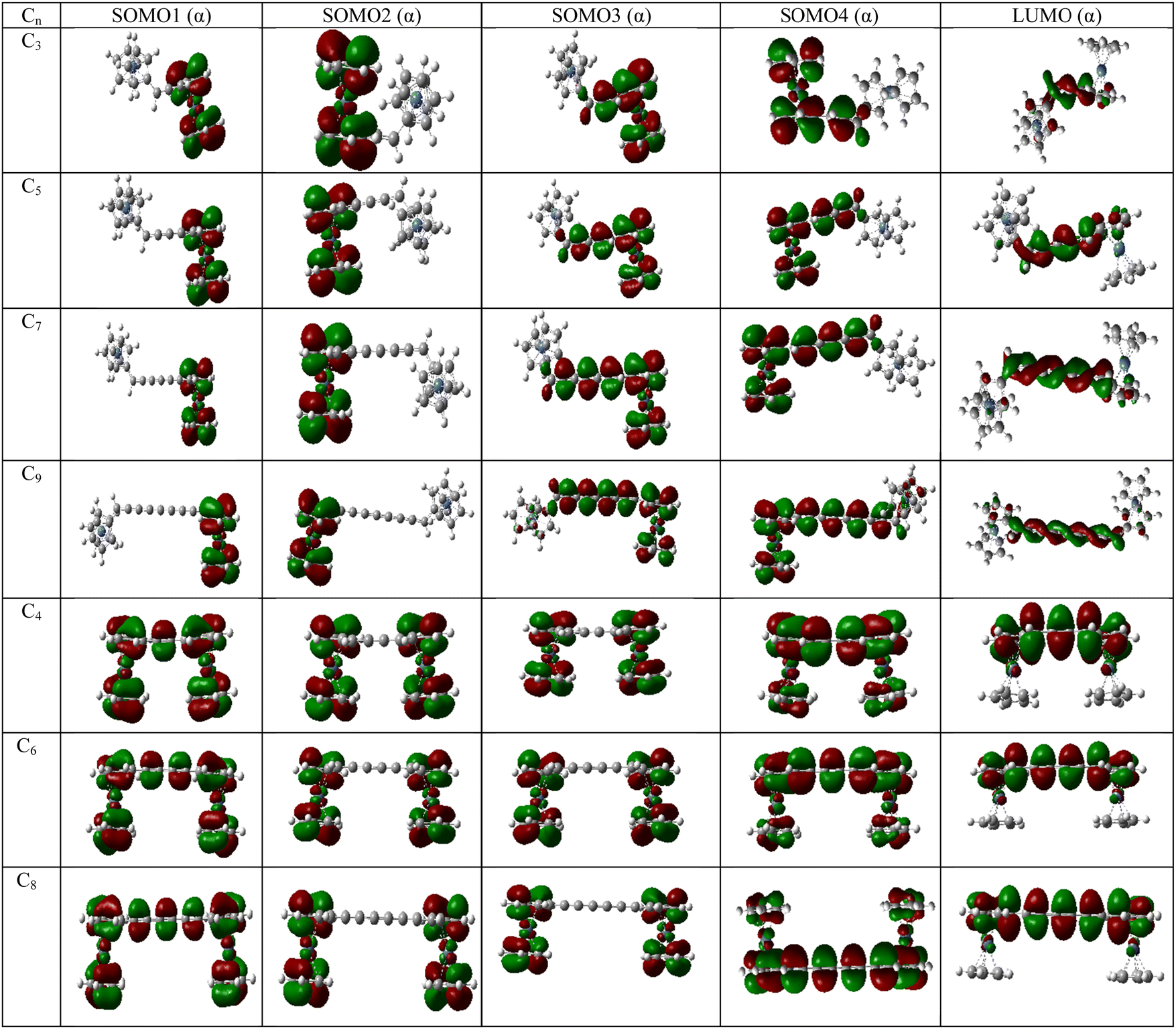 | ||
| Fig. 6 Frontier molecular orbitals of [Ni]–Cn–[Ni] complexes in their high-spin state (quintet) [UB3LYP/6-311++g(d,p)]. The order of energy of the MOs is ESOMO1 < ESOMO2 < ESOMO3 < ESOMO4 < ELUMO. | ||
Zero-field splitting parameter (ZFS)
The energy barrier (U) for the reversal of magnetization depends on zero-field splitting parameter (D) and the ground-state spin (S) of a system. Hence, the increase in ground state spin should result in an increase in energy barrier (U) for spin reorientation. However, with the increase in ground state spin, the ZFS parameter decreases which leads to a decrease in the U value.50 Therefore, the ZFS parameter is the determining factor for large U values. A significant negative value of ZFS (D) parameter of a high-spin (S) ground state causes the spin to point towards a preferred easy-axis, which results in the single-molecule magnet behaviour of a system, whereas systems with positive D values are not suitable candidates for SMMs and the type of anisotropy of these systems is known as easy-plane anisotropy. The calculated values of zero-field splitting parameter (D) for the systems with ferromagnetic ground state are given in Table 10.| System | D (cm−1) | |
|---|---|---|
| [Ni]–Cn–[Ni] | C3 | −2.758 |
| C5 | −2.712 | |
| C7 | −2.654 | |
| C9 | −2.550 | |
| [Cr]–Cn–[Cr] | C3 | 0.350 |
| C5 | 0.351 | |
| C7 | 0.373 | |
| C9 | 0.405 | |
| [Cr]–Cn–[Ni] | C4 | 2.158 |
| C6 | 1.922 | |
| C8 | 1.380 | |
From Table 10, we can see that [Ni]–Cn–[Ni] systems with ferromagnetic ground state have considerable negative D values, whereas [Cr]–Cn–[Cr] and [Cr]–Cn–[Ni] systems have positive D values. Furthermore, for [Ni]–Cn–[Ni] and [Cr]–Cn–[Ni], the absolute value of D decreases with the increase in coupler length. However, in case of [Cr]–Cn–[Cr], the D values increase with the increase in coupler length. To explain this, we have examined the individual excitation contribution to the D value (Table 11). As the chain length increases, it donates increasing density to Ni centers. As a result, this donation decreases the open-shell character on Ni locally. This leads to smaller spin–orbit couplings and smaller ZFS. For Cr, the opposite situation happens since Cr is more donating.
| Complexes | SOMO–VMO (α → α) | DOMO–SOMO (β → β) | SOMO–SOMO (α → β) | DOMO–VMO (β → α) | |
|---|---|---|---|---|---|
| [Ni]–Cn–[Ni] | C3 | −0.28504 | −1.59211 | −0.97555 | 0.47731 |
| C5 | −0.27790 | −1.57731 | −0.96742 | 0.48342 | |
| C7 | −0.26792 | −1.56192 | −0.95361 | 0.48962 | |
| C9 | −0.25322 | −1.52350 | −0.92813 | 0.49739 | |
| [Cr]–Cn–[Cr] | C3 | −0.12238 | 0.21049 | −0.00043 | 0.26703 |
| C5 | −0.11602 | 0.21259 | −0.00059 | 0.25844 | |
| C7 | −0.10273 | 0.21577 | −0.00152 | 0.26348 | |
| C9 | −0.08775 | 0.22284 | −0.00295 | 0.27220 | |
| [Cr]–Cn–[Ni] | C4 | 0.39807 | 1.25382 | 0.84693 | −0.70950 |
| C6 | 0.34578 | 1.15043 | 0.84530 | −0.76355 | |
| C8 | 0.26671 | 0.91243 | 0.71666 | −0.83939 | |
In Table 11, the contributions of different types of excitations towards ZFS (D) parameter are listed. SOMO, VMO and DOMO represent singly occupied, virtual and doubly occupied molecular orbital respectively. DOMO → SOMO excitations51,52 are found to be the main contributor to the zero-field splitting parameter for [Ni]–Cn–[Ni] and [Cr]–Cn–[Ni] complexes, and it has a similar trend of variation as the ZFS (D) parameter. However, for [Cr]–Cn–[Cr], no considerable trend of variation is observed. Thus, [Cr]–Cn–[Cr] and [Cr]–Cn–[Ni] complexes with ferromagnetic ground state will not behave as a single-molecule magnet because of the presence of easy-plane type of anisotropy. Hence, among all the three types of designed complexes, only [Ni]–Cn–[Ni] systems with ferromagnetic ground state can be considered as suitable candidates for single-molecule magnets.53
Conclusions
In a nutshell, we have chosen nickelocene and chromocene as spin sources for the design of three types of systems, namely, [Ni]–Cn–[Ni], [Cr]–Cn–[Cr] and [Cr]–Cn–[Ni] respectively in this work. A linear Cn chain shows the cumulene type of geometric parameters and, hence, the electronic structure. [Ni]–Cn–[Ni] and [Cr]–Cn–[Cr] systems manifest ferromagnetic interaction for Cn chains with odd numbers of carbon atoms and antiferromagnetic interaction for Cn chains with even numbers of carbon atoms, whereas [Cr]–Cn–[Ni] complexes show ferromagnetic ground state for Cn chains with even numbers of carbon atoms and antiferromagnetic ground state for couplers (Cn chain) with odd numbers of carbon atoms. The spin polarization inside the chromocene moiety was found to be the reason for the reversal of the trend observed for [Ni]–Cn–[Ni] and [Cr]–Cn–[Cr]. Greater accumulation of spin-density, lowered SOMO4 (α) – LUMO (α) gap and increased LUMO population with the increase in linear carbon chain length are the reasons for the increase of magnetic interaction with length. We found a negative zero-field splitting parameter (D) only for [Ni]–Cn–[Ni] complexes among the three types of designed systems and, hence, only [Ni]–Cn–[Ni] systems should be considered as potential candidates for the synthesis of single-molecule magnets.Author contributions:
S. Shil has planned and designed [Ni]–Cn–[Ni] systems and supervised the project. S. Das has planned, designed, and done all calculations for all the considered systems. S. Shil and S. Das have written up this paper. A. Misra has given scientific suggestions and read the manuscript.Conflicts of interest
There are no conflicts to declare.Acknowledgements
S. Shil is thankful to SERB, India for funding through grant no. SRG/2022/000822. A. Misra acknowledges financial assistance from SERB-DST (CRG/2019/000262). S. Das thanks UGC for a fellowship.References
- D. Gatteschi and R. Sessoli, Angew. Chem., Int. Ed., 2003, 42, 268–297 CrossRef CAS PubMed
.
-
D. Gatteschi, R. Sessoli and J. Villain, Molecular Nanomagnets, Oxford University Press, 2006 Search PubMed
- M. Evangelisti, F. Luis, L. J. De Jongh and M. Affronte, J. Mater. Chem., 2006, 16, 2534–2549 RSC
- R. Basler, C. Boskovic, G. Chaboussant, H. U. Güdel, M. Murrie, S. T. Ochsenbein and A. Sieber, Chem. Phys. Chem., 2003, 4, 910–926 CrossRef PubMed
- E. J. L. McInnes, Struct. Bonding, 2006, 122, 69–102 CrossRef CAS
- R. Bircher, G. Chaboussant, C. Dobe, H. U. Güdel, S. T. Ochsenbein, A. Sieber and O. Waldmann, Adv. Funct. Mater., 2006, 16, 209–220 CrossRef CAS
- D. Gatteschi, R. Sessoli and A. Cornia, Chem. Commun., 2000, 725–732 RSC
- G. Aromi and E. K. Brechin, Struct. Bonding, 2006, 122, 1–67 CrossRef CAS
- J. N. Rebilly and T. Mallah, Struct. Bonding, 2006, 122, 103–131 CrossRef CAS
- C. J. Milios, R. Inglis, R. Bagai, W. Wernsdorfer, A. Collins, S. Moggach, S. Parsons, S. P. Perlepes, G. Christou and E. K. Brechin, Chem. Commun., 2007, 3476–3478 RSC
- G. Christou, Polyhedron, 2005, 24, 2065–2075 CrossRef CAS
- G. Christou, D. Gatteschi, D. N. Hendrickson and R. Sessoli, MRS Bull., 2000, 25, 66–71 CrossRef CAS
- E. Coronado and D. Gatteschi, J. Mater. Chem., 2006, 16, 2513–2515 RSC
- J. Tejada, E. M. Chudnovsky, E. Del Barco, J. M. Hernandez and T. P. Spiller, Magnetic qubits as hardware for quantum computers, 2001, vol. 12.
-
A. Cornia, A. F. Costantino, L. Zobbi, A. Caneschi, D. Gatteschi, M. Mannini and R. Sessoli, Preparation of Novel Materials Using SMMs, Springer-Verlag, Berlin/Heidelberg, 2006, pp. 133–161 Search PubMed
- J. Gómez-Segura, J. Veciana and D. Ruiz-Molina, Chem. Commun., 2007, 3699 RSC
- B. Cage, S. E. Russek, R. Shoemaker, A. J. Barker, C. Stoldt, V. Ramachandaran and N. S. Dalal, Polyhedron, 2007, 26, 2413–2419 CrossRef CAS
- A. Caneschi, D. Gatteschi, R. Sessoli, A. L. Barra, L. C. Brunel and M. Guillot, J. Am. Chem. Soc., 1991, 113, 5873–5874 CrossRef CAS
- N. Ishikawa, M. Sugita, T. Ishikawa, S. Y. Koshihara and Y. Kaizu, J. Am. Chem. Soc., 2003, 125, 8694–8695 CrossRef CAS PubMed
- Y.-S. Ding, N. F. Chilton, R. E. P. Winpenny and Y.-Z. Zheng, Angew. Chem., 2016, 128, 16305–16308 CrossRef
- C. A. P. Goodwin, F. Ortu, D. Reta, N. F. Chilton and D. P. Mills, Nature, 2017, 548, 439–442 CrossRef CAS PubMed
- K. Kotrle and R. Herchel, Inorg. Chem., 2019, 58, 14046–14057 CrossRef CAS PubMed
- C. Train, L. Norel and M. Baumgarten, Coord. Chem. Rev., 2009, 253, 2342–2351 CrossRef CAS
- M. E. Ali and S. N. Datta, J. Phys. Chem. A, 2006, 110, 2776–2784 CrossRef CAS PubMed
- V. Polo, A. Alberola, J. Andres, J. Anthony and M. Pilkington, Phys. Chem. Chem. Phys., 2008, 10, 857–864 RSC
- S. Shil, M. Roy and A. Misra, RSC Adv., 2015, 5, 105574–105582 RSC
- C. H. Hendon, D. Tiana, A. T. Murray, D. R. Carbery and A. Walsh, Chem. Sci., 2013, 4, 4278–4284 RSC
- X. Gu, R. I. Kaiser and A. M. Mebel, ChemPhysChem., 2008, 9, 350–369 CrossRef CAS PubMed
- D. R. Taylor, Chem. Rev., 1967, 67, 317–359 CrossRef CAS
- P. Sarbadhikary, S. Shil, A. Panda and A. Misra, J. Org. Chem., 2016, 81, 5623–5630 CrossRef CAS PubMed
- S. Shil and S. Sen, Inorg. Chem., 2020, 59, 16905–16912 CrossRef CAS PubMed
- L. Noodleman, J. Chem. Phys., 1981, 74, 5737–5743 CrossRef CAS
- L. Noodleman and E. R. Davidson, Chem. phys., 1986, 109, 131–143 CrossRef
- K. Yamaguchi, H. Fukui and T. Fueno, Chem. Lett., 1986, 625–628 CrossRef CAS
- K. Yamaguchi, Y. Takahara, T. Fueno and K. Nasu, Jpn. J. Appl. Phys., 1987, 26, L1362–L1364 CrossRef CAS
- K. Yamaguchi, F. Jensen, A. Dorigo and K. N. Houk, Chem. Phys. Lett., 1988, 149, 537–542 CrossRef CAS
- K. Yamaguchi, Y. Takahara, T. Fueno and K. N. Houk, Theor. Chim. Acta, 1988, 73, 337–364 CrossRef CAS
- W. Wernsdorfer and R. Sessoli, Science, 1999, 284, 133–135 CrossRef CAS PubMed
- C. E. Dubé, R. Sessoli, M. P. Hendrich, D. Gatteschi and W. H. Armstrong, J. Am. Chem. Soc., 1999, 121, 3537–3538 CrossRef
- T. Goswami and A. Misra, Chem. – Eur. J., 2014, 20, 13951–13956 CrossRef CAS PubMed
- S. K. Singh and G. Rajaraman, Chem. – Eur. J., 2014, 20, 5214–5218 CrossRef CAS PubMed
-
M. J. Frisch, G. W. Trucks, H. B. Schlegel, G. E. Scuseria, M. A. Robb, J. R. Cheeseman, G. Scalmani, V. Barone, G. A. Petersson, H. Nakatsuji, X. Li, M. Caricato, A. V. Marenich, J. Bloino, B. G. Janesko, R. Gomperts, B. Mennucci, H. P. Hratchian, J. Ortiz, A. F. Izmaylov, J. L. Sonnenberg, D. Williams-Young, F. Ding, F. Lipparini, F. Egidi, J. Goings, B. Peng, A. Petrone, T. Henderson, D. Ranasinghe, V. G. Zakrzewski, J. Gao, N. Rega, G. Zheng, W. Liang, M. Hada, M. Ehara, K. Toyota, R. Fukuda, J. Hasegawa, M. Ishida, T. Nakajima, Y. Honda, O. Kitao, H. Nakai, T. Vreven, K. Throssell, J. A. Montgomery Jr., J. E. Peralta, F. Ogliaro, M. J. Bearpark, J. J. Heyd, E. N. Brothers, K. N. Kudin, V. N. Staroverov, T. A. Keith, R. Kobayashi, J. Normand, K. Raghavachari, A. P. Rendell, J. C. Burant, S. S. Iyengar, J. Tomasi, M. Cossi, J. M. Millam, M. Klene, C. Adamo, R. Cammi, J. W. Ochterski, R. L. Martin, K. Morokuma, O. Farkas, J. B. Foresman and D. J. Fox, Gaussian 16, Revision B.01, 2016 Search PubMed
- F. Neese, Wiley Interdiscip. Rev.: Comput. Mol. Sci., 2012, 2, 73–78 CAS
- S. Shil and C. Herrmann, J. Comput. Chem., 2018, 39, 780–787 CrossRef CAS PubMed
- S. Puhl, T. Steenbock, C. Herrmann and J. Heck, Angew. Chem., Int. Ed., 2020, 59, 2407–2413 CrossRef CAS PubMed
- C. Trindle and S. N. Datta, Int. J. Quantum Chem., 1996, 57, 781–799 CrossRef CAS
- C. Trindle, S. N. Datta and B. Mallik, J. Am. Chem. Soc., 1997, 119, 12947–12951 CrossRef CAS
- C. Herrmann, J. Neugebauer, J. A. Gladysz and M. Reiher, Inorg. Chem., 2005, 44, 6174–6182 CrossRef CAS PubMed
- P. Sarbadhikary, S. Shil and A. Misra, Phys. Chem. Chem. Phys., 2018, 20, 9364–9375 RSC
- O. Waldmann, Inorg. Chem., 2007, 46, 10035–10037 CrossRef CAS PubMed
- J. Cirera, E. Ruiz, S. Alvarez, F. Neese and J. Kortus, Chem. – Eur. J., 2009, 15, 4078–4087 CrossRef CAS PubMed
- F. Neese and E. I. Solomon, Inorg. Chem., 1998, 37, 6568–6582 CrossRef CAS PubMed
- C. E. Dubé, R. Sessoli, M. P. Hendrich, D. Gatteschi and W. H. Armstrong, J. Am. Chem. Soc., 1999, 121, 3537–3538 CrossRef
Footnotes |
| † This work is dedicated to Professor Douglas J Klein on the occasion of his 80th birthday. |
| ‡ Electronic supplementary information (ESI) available: Bond angles and optimized coordinates calculated in UB3LYP/6-311++g(d,p) methodology. Bond angles, bond lengths and spin density distributions calculated in MN12SX/6-311++g(d,p) level of theory. 〈S2〉BS and 〈S2〉HS values calculated in UB3LYP/6-311++g(d,p) and UMN12SX/6-311++g(d,p) methodologies are provided. Molecular orbital pictures are given. The HOMO-LUMO gap of the complexes at UB3LYP/6-31g(d,p) level of theory are given. See DOI: https://doi.org/10.1039/d3cp00194f |
| This journal is © the Owner Societies 2023 |