
Can graphene improve the thermal conductivity of copper nanofluids?†
Gabriel J.
Olguín-Orellana
 a,
Germán J.
Soldano
b,
Jans
Alzate-Morales
a,
María B.
Camarada
*cd and
Marcelo M.
Mariscal
*b
a,
Germán J.
Soldano
b,
Jans
Alzate-Morales
a,
María B.
Camarada
*cd and
Marcelo M.
Mariscal
*b
aCenter for Bioinformatics, Simulation and Modeling (CBSM), Faculty of Engineering, Universidad de Talca, 1 Poniente 1141, Talca, Chile
bINFIQC, CONICET, Departamento de Química Teórica y Computacional, Facultad de Ciencias Químicas, Universidad Nacional de Córdoba, Argentina. E-mail: marcelo.mariscal@unc.edu.ar
cLaboratorio de Materiales Funcionales, Departamento de Química Inorgánica, Facultad de Química y de Farmacia, Pontificia Universidad Católica de Chile, Chile
dCentro Investigación en Nanotecnología y Materiales Avanzados, CIEN-UC, Pontificia Universidad Católica de Chile, Santiago, Chile. E-mail: mbcamara@uc.cl
First published on 21st January 2023
Abstract
Copper (Cu) nanofluids (NFs) have attracted attention due to their high thermal conductivity, which has conferred a wide variety of applications. However, their high reactivity favors oxidation, corrosion and aggregation, leading them to lose their properties of interest. Copper capped by graphene (Cu@G) core@shell nanoparticles (NPs) have also attracted interest from the medical and industrial sectors because graphene can shield the Cu NPs from undesired phenomena. Additionally, they share some properties that expand the range of applications of Cu NFs. In this work, new Morse potentials are reported to reproduce the behavior of Cu@G NPs through molecular dynamics. Coordination-dependent Morse parameters were fitted for C, H, and Cu based on density functional theory calculations. Then, these parameters were implemented to evaluate the thermal conductivity of Cu@G NFs employing the Green–Kubo formalism, with NPs from 1.5 to 6.1 nm at 100 to 800 K, varying the size, the number of layers and the orientation of the graphene flakes. It was found that Cu@G NFs are stable and have an improved thermal conductivity compared to the Cu NFs, being 3.7 to 18.2 times higher at 300 K with only one graphene layer and above 26.2 times higher for the graphene-trilayered NPs. These values can be higher for temperatures below 300 K. Oppositely, the size, homogeneity and orientations of the graphene flakes did not affect the thermal conductivity of the Cu@G NFs.
1 Introduction
During the last few decades, nanofluids (NFs), which are colloidal suspensions of nanoparticles (NPs) that significantly optimize the applications of the base fluids, have attracted wide-spread attention due to their exceptionally high thermal conductivity (κ), thermal diffusivity and convective heat transfer coefficients at low NP volume fractions.1–5 Although solid particles of micrometer and millimeter sizes have been added to fluids to improve their properties, practical uses for these colloids have been limited because the particles settle rapidly, clogging flow channels, eroding and causing severe pressure drops.5–8In particular, copper (Cu) NFs have been studied for their potential applications in diverse medical and industrial activities, including chemical engineering, refrigeration, transportation, energy production and distribution, and electronics.4,9 In these applications, the κ of the cooling fluids plays a vital role in developing energy-efficient heat transfer equipment, but conventional one-phase fluids like ethylene glycol, propylene glycol, kerosene, oils, and water have poor heat transfer properties.5,10 These fluids possess a κ three to four orders of magnitude lower than metals such as silver and Cu or carbon-based materials such as graphene and carbon nanotubes.11,12 This reason has led researchers to focus on elucidating the factors affecting the thermophysical properties of the Cu NFs, where volume, concentration, temperature, size, and shape of the NPs have been suggested as the most important.5,11–15 However, investigations have not been conclusive due to the difficulty of measuring the κ of NPs and because the mechanisms influencing heat transfer in NFs have not been clarified. Other factors, such as the preparation technique, stabilizing agents, air-exposure time, flow characteristics and acidity of the NF have also been described as relevant.6,7,14–19
For example, Bhanushali et al. investigated how the shape of the NPs determines the κ of water-based Cu NFs using distinct filler particles: short nanowires (mean diameter (Dm) = 26 nm; mean length (Lm) = 7.8 μm), long nanowires (Dm = 26 nm; Lm = 96 μm), nanospheres (Dm = 48 nm), and nanocubes (Dm = 87 nm). The NPs were treated with the same dispersant and antioxidant to exclude the potential effects of the surface-capping ligands. In all cases, the results indicate an increment in the κ with the loading of the NPs, but going from 4.2% for the nanocubes to 40% for the long nanowires at 0.25 vol%.11 On the other hand, Qiang et al. investigated the convective heat transfer and flux characteristics of Cu NFs in a tube. The samples were prepared by mixing Cu NPs with diameters below 100 nm and deionized water and fatty acid salts as dispersants. The results show that the NPs remarkably increase the convective heat transfer of the base fluid as a function of the concentration of NPs, reaching an increment of about 60% at 2.0 vol% of Cu NPs.6 As was mentioned, little variation in the size and loading of the NPs can lead to great changes in the κ of the NFs.
Generally, NFs with small NPs have superior heat transfer properties than conventional fluids and those containing microscopic particles because the heat transfer occurs at the surface of the NPs.14,20 Additionally, the small size has been reported as a factor that increases the stability of suspensions.5,8,15 However, this cannot be expected for Cu NFs, because Cu NPs of small size are highly reactive and oxidized, corroded and aggregated quickly, leading to the NFs losing their improved thermophysical properties.17,21–25 This phenomenon was evidenced by Liu et al., who reported the κ of Cu–water NFs with NPs of different sizes and shapes, and concentrations. The greatest improvement concerning the pure water was 23.8%, obtained with spherical and cubic NPs of 50 to 100 nm at 0.1 vol%. No higher values of the κ were measured, even for higher concentrations or sizes of the NPs. Furthermore, as no surfactants and dispersants were used, the κ was time-dependent, decreasing to a value similar to the water after 10 minutes.14 According to this evidence, proper ways to prevent oxidation and aggregation of the Cu NPs and manage the events on their surface must be developed. Therefore, covering the NPs with another stabilizing material is one of the most promising alternatives.11,26
Recently, graphene-capped copper (Cu@G) NPs have attracted research and commercial interest because graphene can serve as a shield to protect the Cu NPs and enhance their thermal, optical, structural, catalytic, and conductive properties.22,27–33 Furthermore, carbon-derived materials are ideal candidates for coating compared with other materials: (i) they are stable in acidic and alkaline solutions; (ii) different types of functional groups can be attached to their surface by oxidation; (iii) the functional groups in the carbon shell can be used to induce further coating and to obtain ternary hybrid structures; and (iv) carbon is also an excellent electrical and thermal conductor.34,35
Carbon-based materials have been proposed as nanofillers due to their remarkable thermal properties.11 Different studies have suggested that the κ of graphene and carbon nanotubes are in the range of 1950–6500 W m−1 K−1 at room temperature, which are values among the highest known.36 As NFs, they present a κ even greater than those predicted by theories and models. In 2001, Choi et al. reported that for a nanotube loading of and below 0.3 volume fraction in oil, the κ ratio is similar to Cu NPs in the same fluid. However, the nanotubes have a higher enhancement at 0.5 vol%, with the κ ratio exceeding 1.5 and more than 2.5 at ∼1 vol%. This study demonstrated that the increment in κ is nonlinear with the nanotubes content, while all theoretical predictions exposed a linear relationship.13 In addition, graphene-water NFs were investigated as heat sinks, resulting in an increment in the convective heat transfer that reached ∼84%;37 in a heat pipe, graphene nanosheets were reported to enhance the κ of water by ∼28%;38 and even a greater improvement was quantified for ethylene glycol, where dispersed graphene increased the κ by up to 86% at 5.0 vol%.39
Although some studies have provided methods to produce Cu@G heterostructures,40–53 their diameter, size distribution, shape, and the number of graphene capping layers remain uncontrollable. These properties depend on many factors, which are hard to manipulate during the synthesis process. Furthermore, they can change during the usage of the NPs, especially if submitted to mechanical, heat, and pressure regimes.
These reasons have hindered the exploration of Cu@G NPs as a nanofiller and, to our knowledge, only one article has been reported regarding this topic.54 In that work, the thermal properties of Cu@G–water NFs were estimated when varying the loading fraction of NPs, at different temperatures under 45 °C. The addition of the NPs appears to positively affect the heat transfer of the NFs when the temperature increases, with an improvement in the κ going from 9% at 30 °C and a concentration of 0.1 w% to 15% at 40 °C and 0.05 w%. These results can be encouraging but limited because some factors could not be managed during the synthesis of the NPs, such as the size distribution and the number of layers of graphene covering the NPs. Then, more studies are necessary to advance to conclusive results.
To date, many efforts have been made to explain the mechanisms behind the κ enhancement in NFs, through various methodologies and assumptions.1,7,13,15,16,55 However, more studies are necessary to understand how each factor influences the structural, thermodynamic, reactive, and mechanical properties of the Cu@G NPs and to quantify their contribution to the improvement of the κ of Cu@G-based NFs. In addition to the experimental techniques, high-performance computing-assisted materials design has proved to be a powerful tool for gathering insight from different physical phenomena.2,7,19,30,56–65 It represents a powerful way to predict the feasibility and properties of a system that cannot be accessed by other means, saving preparation time, effort, and costs.
In this work, we studied the effect on κ caused by adding graphene layers to Cu NPs and by employing computer simulations with Morse potentials developed in our group. Equilibrium molecular dynamics (EMD) simulations based on the Green–Kubo formalism were employed to study the κ of Cu and Cu@G NPs in an Argon (Ar) fluid, a strategy already reported for pure Cu NFs.2,7,65–67 In our study, we considered six key factors to quantify the contribution to the enhancement of the κ: (i) the size of the Cu NPs; (ii) the presence of graphene flakes; (iii) the number and size of graphene flakes surrounding the Cu NPs; (iv) the number of layers covering the Cu NPs; (v) the initial orientation of the flakes towards the surface of the Cu NPs and; (vi) the temperature of the systems.
The results indicate that Cu@G NFs are stable and have an improved thermal conductivity compared to NFs with bare Cu NPs, a property that increases with the number of graphene layers covering the NPs and decreases with the temperature. On the other hand, the size, homogeneity and orientation of the graphene flakes at the Cu surface do not affect this property.
2 Methodology
2.1 Density functional theory calculations
Density functional theory (DFT) calculations were performed through the Quantum Espresso/PWSCF.68 The Perdew–Burke–Ernzerhof (PBE) generalized gradient approximation functional is the most popular exchange–correlation functional in DFT for materials science69,70 because of its reasonable accuracy over a wide range of systems and its low computational cost. It was adopted for the exchange–correlation term using the high-throughput GBRV pseudopotentials,71 with kinetic energy cut-offs of 40/200 Ry for the wave-function/charge density, respectively. A Gaussian spreading of 0.01 Ry was employed. The long-range van der Waals interactions were accounted for utilizing the DFT-D3 approach,72 which has shown to be remarkably accurate for similar systems such as graphene on Au (111) and Ag (111).73 Cell dimensions were chosen that were large enough so that the NPs were at least 10 Å from their periodic images. Geometry relaxations converged when forces acting on atoms were weaker than 0.01 eV Å−1. The gamma point was selected to sample the Brillouin zone. Spin polarization was considered for a few configurations showing neither magnetization nor energy difference concerning not polarized calculations. Therefore, the latter approach was used.2.2 Development of a coordination-dependent Morse potential
Morse potentials were developed to reproduce the Cu–C and Cu–H interactions according to the equation| E(r) = De(1 − e−α(r−re)) | (1) |
Performing DFT calculations for the whole Cu NPs and graphene flakes would be unfeasible in terms of computational costs. Instead, starting from a 1.5 nm Cu NP, we considered only the first three layers of a (100) and a (111) face. On top of each surface, we added a relaxed graphene flake large enough to cover the Cu NP completely, as shown in Fig. 1(a). Several single-point energies were calculated, corresponding to different heights and lateral displacements of the flakes to the surfaces, for both planar and curved flakes. The corresponding adsorption energies are plotted in Fig. 1(b), and the complete list of configurations considered is given in the ESI† (see DFT-scf-Configurations.xyz). These DFT values were employed to fit three Morse potentials: C–Culow, C–Cuhigh, and H–Cu (Table 1), where Culow are the Cu atoms with a coordination number ≤8 and Cuhigh are those with a coordination number ≥9 and ≤12. As was expected, the potential well depth for C–Culow is considerably more profound than for C–Cuhigh, since Cu atoms with coordination ≤8 are more reactive than those with higher coordination. The single point energies calculated with these Morse potentials are also plotted in Fig. 1(b), and are in good agreement with the DFT calculations.
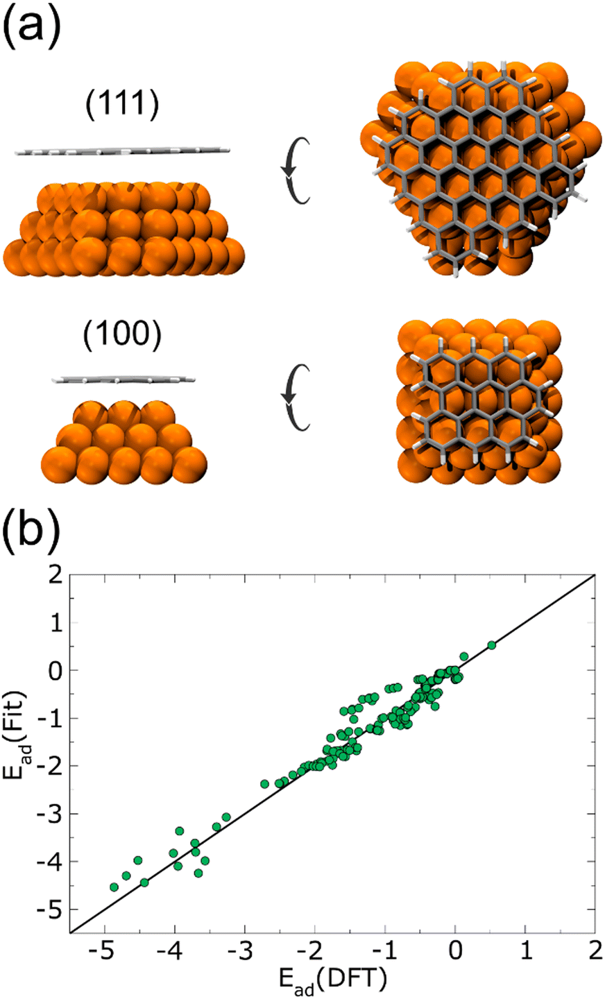 | ||
| Fig. 1 (a) Side and top views of 2 of 193 nanostructures on several sites, heights, and configurations on the surfaces used to model the flake-Cu NP interaction for the Morse potential fitting. The (111) and (100) faces of the Cu NP were considered, shown at the top and bottom, respectively. (b) Adsorption energies for each one of the 193 nanostructures. DFT and fitted Morse values are compared. | ||
| D e (eV) | α (Å−1) | r (Å) | |
|---|---|---|---|
| Culow–C | 3.56311053 × 10⁻² | 1.43902338 | 2.40244842 |
| Cuhigh–C | 8.99999961 × 10⁻³ | 1.09784114 | 4.11547661 |
| Cu–H | 3.5631105 × 10⁻² | 1.43902338 | 2.40244842 |
2.3 Starting configurations for thermal conductivity calculations
As initial configurations, five Cu NPs of 1.5, 2.3, 3.1, 4.0, and 6.1 nm diameter were built, following the Wulff construction for highly symmetric face-centered cubic (FCC) metals conforming a truncated octahedron, which is the most stable shape for Cu NPs in vacuum conditions.74 Next, five Cu@G NPs models were generated using the same Cu NPs surrounded by 14 zigzag square graphene flakes, considering that the sum of their areas was enough to cover the whole NP. These models were labeled according to their size, adding the suffix G14 to those capped by graphene. The uncapped and capped NP models (after relaxation) are shown in Fig. 2(a). In order to simulate the nanofluid, they were put into Ar with a box dimension of the NP diameter plus 20 Å in each direction of the three-dimensional space and an Ar density ρ = 1418 kg m−3, with periodic boundary conditions in all directions, following the configuration suggested by Sarkar & Selvam,7 and Kang et al.2 Finally, they were relaxed to reduce the steric hindrances and to obtain NF systems such as those exemplified in Fig. 2(b).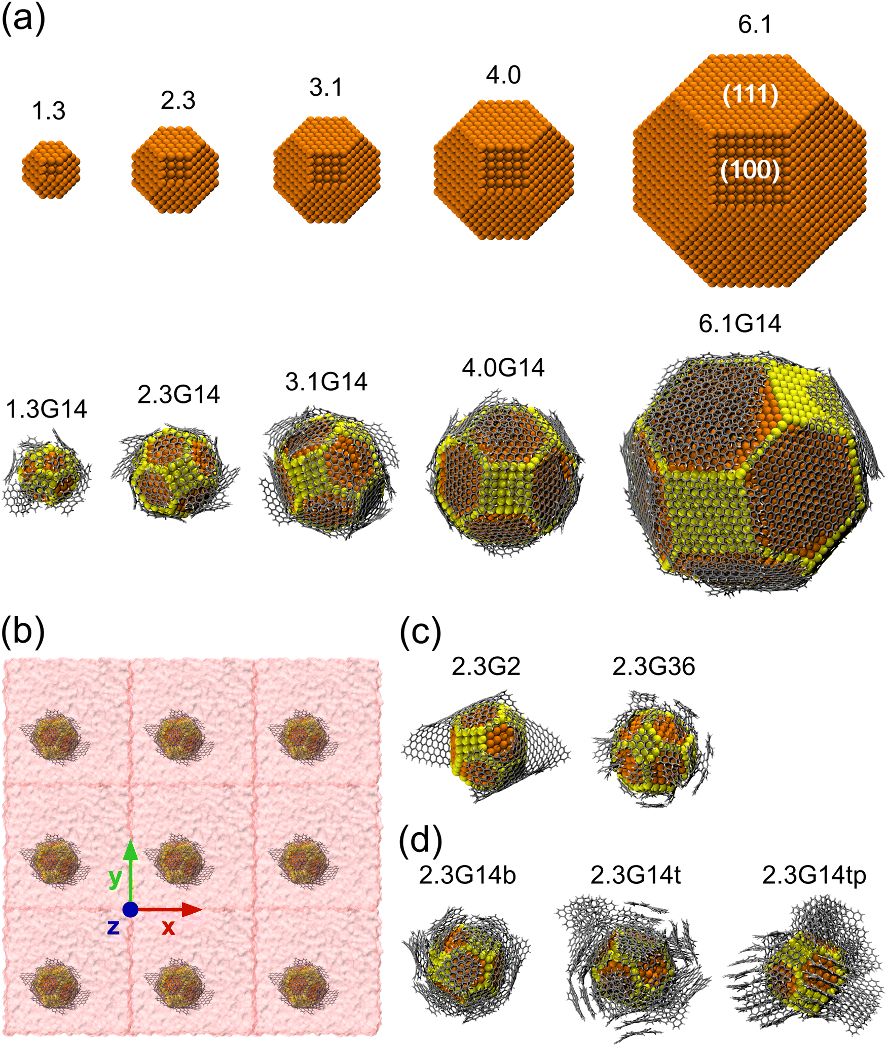 | ||
| Fig. 2 (a) Main capped and uncapped Cu NP models, named according to their diameters in nm and their number of graphene flakes. The (111) and (100) faces of the Cu NP are labeled in 6.1. The yellow spheres represent the Cu atoms with a coordination number ≤8 (Culow) and the orange ones with a coordination number ≥9 and ≤12 (Cuhigh). (b) Simplified model of the 2.3G14 NF with PBC. (c) Simulation models to evaluate the effect of the size of the flakes and (d) the number of graphene layers used in the estimation of κ for NFs. The Argon boxes were hidden to facilitate the visualization. | ||
Five new model systems were constructed from the Cu NP of 2.3 nm. Two of them, 2.3G2 and 2.3G36, which have 2 and 36 graphene flakes each (Fig. 2(c)), were used to explore the effect of changing the size of the flakes but with the same number of carbon atoms as 2.3G14. The other three (Fig. 2(d)), 2.3G14b (b = bilayer, 2.3G14t (t = trilayer), and 2.3G14tp (tp = trilayer perpendicular), were used to understand how the quantity of layers and their initial orientation does affect the κ of the NFs.
Three additional systems were built (Fig. S1, ESI†) to understand the contribution of each nanomaterial to the κ. In the first one, considering that the Ar box in 2.3G14 was bigger than in 2.3, to be able to compare the κ of 2.3 and 2.3G14, a new 2.3 NF model with an Ar box having the same size as 2.3G14 was generated. This model was named 2.3e. In the second one, 14 graphene flakes (like those in 2.3G14) were randomly distributed into an Ar box with equal dimensions to 2.3G14 and called G2.3 × 14. In the last one, a single graphene flake was simulated in a box with 1/14 of the volume and Ar atoms than G2.3 × 14. This last model was built to study the behavior of the graphene flakes avoiding the aggregation phenomena.
All these new NP models were relaxed and were placed into an Ar box following the same procedure mentioned above. This schema was also replicated for a mono-, bi- and trilayer infinite graphene, the κ of which has been measured and calculated through different techniques,36,75–79 to have the reported values as a reference to corroborate the accuracy of our methodology. Ar was added only in the plane perpendicular to the surface in this case. A summary of the dimensions of the systems and their atomic composition is exposed in Table S1 (ESI†).
2.4 Molecular dynamics
For the Cu NF systems, the embedded atom method (EAM) potentials developed by Foiles80 were used to reproduce the Cu–Cu interactions. At the same time, the Lv's19 and Fraenkel's81 Lennard-Jones (LJ) parameters were set out for the Cu–Ar and Ar–Ar interactions, respectively. In the case of the Cu@G NFs, Akiner et al. concluded82 that the potential parameters of the interface should be carefully optimized to correctly simulate heat transport for solid–liquid systems when using the Green–Kubo method. Therefore, Morse potentials were developed to calculate the Cu–C and Cu–H energies and forces. The procedure to generate these parameters from DFT calculations is described below. The Cu–Cu, Cu–Ar and Ar–Ar interactions were studied with the same parameters previously mentioned, and Stuart's adaptive intermolecular reactive bond order (AIREBO) force field83 was applied to consider the behavior of the graphene flakes. Two extra LJ parameters were used for the C–Ar and H–Ar interactions, taken from Fraenkel's study in which the Ar–Ar potential was developed.81Ar has been chosen as the base fluid in most MD simulation studies on NFs due to its well-defined LJ potentials and simplicity. These potentials employ a simple two-body form that requires much less calculation time than more complex potentials involving other terms.7 Previous studies that used MD to compute the properties of NFs have proved that the potential functions effectively indicate their intermolecular interactions.2,19,66,84–86 A summary of the used LJ parameters taken from the literature is shown in Table S2 (ESI†). In all the calculations, the cut-offs were 3.0 Å for the AIREBO potential and 13.0 Å for the LJ and Morse's interactions.
All MD simulations were performed in LAMMPS,87 using a canonical (NVT) ensemble and periodic boundary conditions (PBC) in all planes. The models were energetically minimized using the Polak-Ribiere version of the conjugate gradient algorithm88 with a tolerance for the energy of 1.0 × 10⁻⁹ and the force equal to 1.0 × 10⁻¹⁰ eV Å−1. Then, 50 ps of thermalization and 1 ns of production were done using a time step of 1 fs. Temperatures from 100 to 800 K in intervals of 100 K were sampled using the Nose–Hoover thermostat with a Tdamp of ten times the time step value, repeating each simulation six times to obtain averaged energies and structural properties.
2.5 Thermal conductivity calculations
The thermal conductivity (κ) is a measure of the propensity of a material to transmit heat energy in a diffusive manner. It is defined as a linear coefficient relating the macroscopic heat current vector to the temperature gradient as given by Fourier's law:
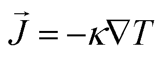 | (2) |
 is the heat flux in units of energy per area per time and ∇T is the spatial gradient of temperature.
The total thermal conductivity κ can be written as:
| κ = κe + κl | (3) |
κ l is estimated by means of the Green–Kubo formalism, meanwhile κe, which is very relevant for metals, can be estimated by using the Wiedemann–Franz (WF) equation for simple metals as:
| κe ≈ TL0σ | (4) |
For Cu NPs with an average size of 20 nm (a bit larger than ours), and based on its experimental value for electrical conductivity,89 the electronic contribution in thermal conductivity can be estimated as κe ≈ 300 K × 2.44 × 10−8 W Ω2 K−2 × 5 × 106 Ω−1 m−1 = 36.6 W m−1 K−1 that is expected to decrease for smaller sized NPs.
Recent studies confirmed a dramatic decrease in the electrical conductivity and κ when the dimension is comparable to or smaller than the electron mean free path. However, verifying the Wiedemann–Franz law in these nanostructures remains hotly debated.90
Non-equilibrium molecular dynamics (NEMD) and equilibrium molecular dynamics (EMD) can be used to calculate the heat transport properties computationally. In NEMD, a heat flux is imposed on the system and the κl is calculated based on the resulting temperature gradients. However, finite-size effects require careful considerations to obtain reliable temperature profiles. Additionally, EMD calculates κl from the time decay of heat flux fluctuations based on the fluctuation–dissipation theorem, through the fluctuations of the per-atom potentials and kinetic energies and the per-atom stress tensor in a steady-state equilibrated simulation. Despite requiring more computational power, this method does not suffer from the drawbacks of NEMD and is widely used in the literature.2,7,65,67,91,92 More details about how to calculate the κ of molecular systems via EMD through the Green–Kubo formalism can be found in Appendix A.
3 Results and discussion
The accuracy of the employed method was validated by comparing the κ of liquid Ar with previously reported theoretical and experimental data at its steady point T = 86 K and ρ = 1418 kg m−3.2,7,84,85 We varied the simulation time from 0.25 ns to 1 ns and the edges of the simulation box from 30 to 60 Å. The results (Table S3, ESI†) indicate that the κ for these models is in an acceptable margin compared to the experimental value of 0.132 W m−1 K−1![[thin space (1/6-em)]](https://www.rsc.org/images/entities/char_2009.gif) 93 and compared with theoretical calculations.94 Similar simulations were performed for infinite graphene of one, two and three layers. The results are presented in Fig. S2 (ESI†). They show that κ decreases exponentially with the temperature, going from 10410 W m−1 K−1 at 100 K to 1612 W m−1 K−1 at 800 K for the case of the monolayer of graphene. At 300 K, the average value was 3643 W m−1 K−1, which agrees with the reported experimental value ∼4000 W m−1 K−136,75–77 and the DFT calculations.78,79 Furthermore, it is suggested that the κ for the same amount of material decreases as the number of layers increases, a conclusion that other authors have also reported.95,96
93 and compared with theoretical calculations.94 Similar simulations were performed for infinite graphene of one, two and three layers. The results are presented in Fig. S2 (ESI†). They show that κ decreases exponentially with the temperature, going from 10410 W m−1 K−1 at 100 K to 1612 W m−1 K−1 at 800 K for the case of the monolayer of graphene. At 300 K, the average value was 3643 W m−1 K−1, which agrees with the reported experimental value ∼4000 W m−1 K−136,75–77 and the DFT calculations.78,79 Furthermore, it is suggested that the κ for the same amount of material decreases as the number of layers increases, a conclusion that other authors have also reported.95,96
The dependence of κ of the Cu and Cu@G NFs at different temperatures is shown in Fig. 3(a), together with that reported for bulk copper.97 These results indicate an improved heat transfer capacity for the Cu@G NFs compared to the uncapped ones, which are more remarkable at lower temperatures. As the temperature increases, the decrement of the κ occurs exponentially since, at higher temperatures, more phonons in each vibrational mode are excited, making the collisions between them more intense. In all cases, κ remains higher for the Cu@G compared to the bare NPs systems.
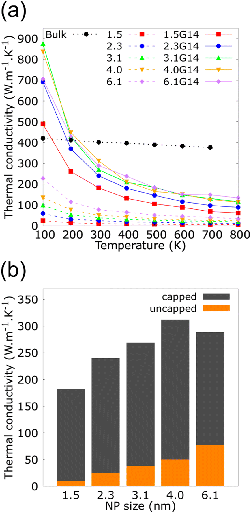 | ||
| Fig. 3 (a) Thermal conductivity (κ) as a function of the temperature for copper–argon nanofluids at different nanoparticle sizes and for copper-graphene-argon nanofluids when the nanoparticles are covered with 14 graphene flakes enough to cover the whole nanoparticle (structures shown in Fig. 2(a)). (b) κ of the same nanofluids at 300 K. | ||
Fig. 3(b) shows the results for the main systems at 300 K, which was the nearest to room temperature. In this case, the increment in the κ of the NFs with capped nanoparticles concerning the uncapped ones was 18.2 times for the 1.5 nm NP, 10 times for the 2.3 nm, 7.1 times for the 3.1 nm, 6.24 times for the 4.0 nm and 3.7 times for the 6.1 nm.
Regarding the structural stability of the NFs, no significant differences in the shape of the NPs and the adsorption mechanisms of the graphene flakes at temperatures under and equal to 500 K were observed. In these cases, the flakes preferably adsorb on the hexagonal (111) faces, probably due to their wider surface, which facilitates the planar interaction. When the (111) faces were covered, they migrated to the (100) (squares) faces or formed multi-layered flakes on the NPs. Shin et al. also reported a better matching between the graphene and Cu (111) surfaces because they have a lattice mismatch of only 3.8% versus 19.9% with respect to the Cu (100) surfaces.98 Then, our results support the proposition of stronger interactions between the graphene and Cu (111) surfaces, and a positive effect on the adsorption. For temperatures higher than 500 K, the NPs of 1.5, 2.3, and 3.1 nm experienced a desorption of some flakes, which form π-stacking interactions mediated by bi- and trilayer structures that remain on the Cu NPs surface but perpendicularly. This desorption phenomenon could be a factor that contributes to the fact that the flakes do not improve the thermal stability of the Cu NPs at higher temperatures (Fig. S3, ESI†), as could be expected for this hybrid nanomaterial due to the well-known high thermal stability of graphene.39,99,100
The consequence of changing the size of the graphene flakes that cover the Cu NP of 2.3 nm is summarized in Fig. 4. These results revealed no significant variations in the κ for the three different NFs containing Cu@G NPs: 2.3G2 (35.4 × 33.3 A2, 828 C atoms), 2.3G14 (14.2 × 13.5 A2, 812 C atoms) and 2.3G36 (9.9 × 8.6 A2, 792 C atoms). Although, the flakes do not homogeneously cover the Cu NPs as in the case of the 2.3G2 NF, or if they are not totally adsorbed on the NPs like in 2.3G36, where the high content of H atoms impedes the adsorption of the flakes. These results could result from maintaining a constant number of atoms in all systems, suggesting that this characteristic of the NPs is more critical for conserving the heat transfer property of the NFs than having a homogeneous coat on the Cu surface.
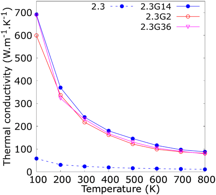 | ||
| Fig. 4 Thermal conductivity (κ) as a function of the temperature for copper–argon and copper-graphene-argon nanofluids (structures shown in Fig. 2(c)) when the copper nanoparticle has a diameter of 2.3 nm and is covered by 14, 2 and 36 graphene flakes enough to cover the whole nanoparticle surface. | ||
Since the synthesis methods of Cu@G NPs reported in the literature have produced multi-layer graphene shells for Cu NPs,41,46–48,53 the variation in the κ concerning the number of layers per flake was studied and reported in Fig. 5. The results indicate that the bi- and trilayered Cu@G NPs have an enhanced κ compared to the NFs with the single-layer Cu@G NP; however, no remarkable increment for the trilayer Cu@G NP model regarding the bilayered Cu@G NP was observed, as could be expected, considering its higher content of graphene.
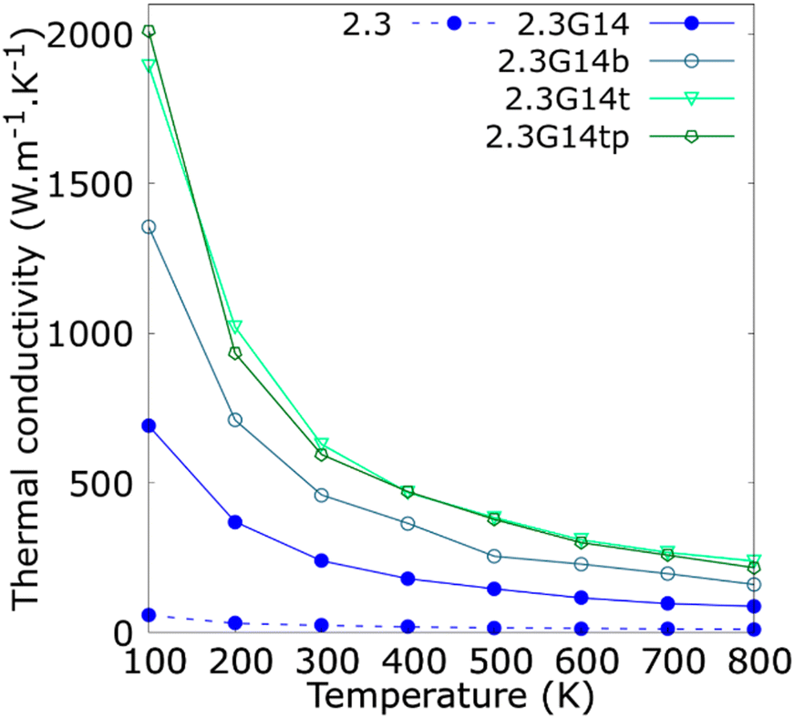 | ||
| Fig. 5 Thermal conductivity (κ) as a function of the temperature for copper–argon and copper-graphene-argon nanofluids (structures shown in Fig. 2(d)) when the copper nanoparticle has a diameter of 2.3 nm and is covered with 14 monolayer, bilayer, trilayer and trilayer perpendicular graphene flakes big enough to cover the whole nanoparticle surface. | ||
Fig. 5 also indicates that the adsorption orientation of the graphene flakes on the Cu surface does not affect the κ of the system. This exciting result suggests the possibility of developing new methods to produce Cu@G NPs. Until now, the reported protocols consist of depositing C atoms on Cu NPs, eventually forming a graphene cover.40,41,46–53 However, to our knowledge, no techniques have been proposed to produce Cu@G NPs in steps, i.e., generating the Cu NPs and graphene flakes separately and then putting them together in a single medium. Our results suggest that, in these cases, it would not matter if the adsorption of the flakes on the NPs occurs planar one by one or if they first form a stack and then adsorb perpendicularly. The κ values of the NFs would not be influenced.
Keblinski et al.101 reported the presence of a solid-like molecular-level layering of the liquid at the surface of the NPs, called the nanolayer, as one of the primary ways influencing the notable improvement of the κ in NFs. Due to the structure of the liquid at the interface remaining more ordered than the bulk fluid, there are possibilities of a larger κ and the ‘tunneling of heat-carrying phonons’ from one particle to another. Since this report was published, diverse experiments and theoretical analyses have been made to characterize the importance of this mechanism in heat transport phenomena. Some of them support this hypothesis, while others conclude that the structured interfacial fluid layer is limited to a few atomic distances from the surface of the NPs, which makes their influence on the thermal transport of the NFs negligible.
Fig. S4 (ESI†) shows the κ for 2.3e, 2.3G14, G2.3 and G2.3 × 14 models, the Ar boxes of which have the same size. The results indicate that the κ of 2.3G14 NF is markedly higher than that of 2.3, and is similar to that of G2.3 and G2.3 × 14. These results suggest that the graphene makes a greater contribution to the κ in these NFs. Meanwhile, the Cu NPs would help to prevent the staking of the flakes and the formation of graphitic structures, which would alter the heat transfer properties of the NF.
Fig. 6 shows the radial distribution functions (RDF) of the nanolayer in the interface of 2.3 (Fig. 6(a)) and 2.3G14 NFs (Fig. 6(b)) at 300 and 800 K. These calculations were performed from the most external Cu atoms of the NPs to the bulk fluid, distinguishing two layers of Ar in the interface: from 0 to 4.0 Å and from 4 to 6.5 Å in 2.3; and from 0 to 8 Å and from 8 to 10.5 Å in 23G14. In this last case, the higher distance for the calculation was set considering the presence of the graphene flakes in the model. For both systems, a higher structuration of the first layer of Ar is observed at 300 K, but it is much more evident on the surface of the uncapped NP. This could be because the uncovered Cu NP has a regular disposition of its external atoms, which eases the arrangement of the fluid at the solid/liquid interface (Fig. 6(c)). On the other hand, the graphene flakes in the 2.3G14 generate interstices in the structure of the NP, which hinders the organization of the Ar in contact with the NP (Fig. 6(d)). At 800 K, none of them reveal the formation of the nanolayer.
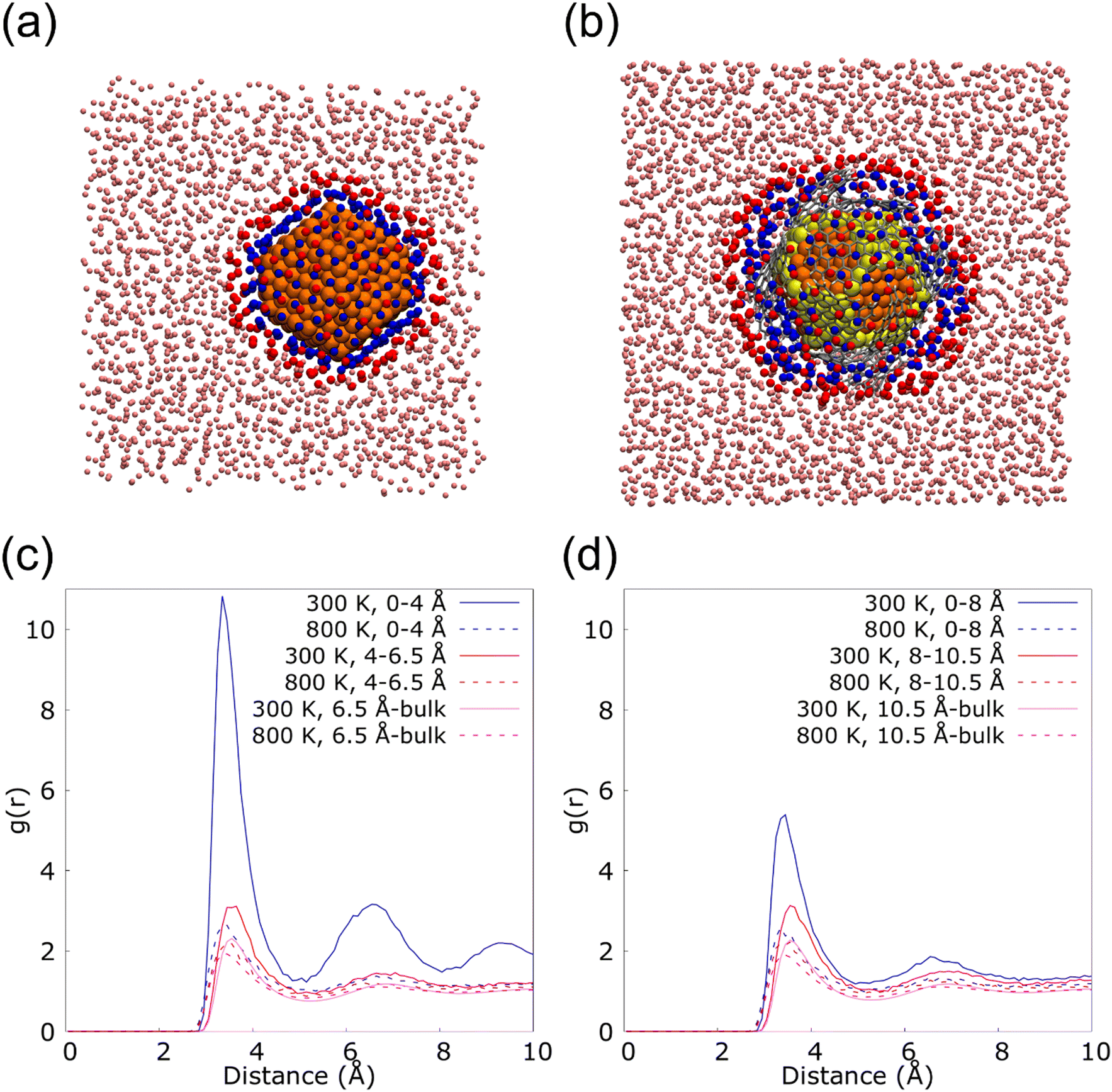 | ||
| Fig. 6 First (blue) and second (red) argon neighbors of the copper nanoparticle of d = 2.3 nm at 300 K when it is (a) uncapped and (b) capped by 14 graphene flakes big enough to cover the whole nanoparticle surface. Radial distribution function (RDF) calculated at 300 and 800 K for the nanofluids containing the (c) uncapped and (d) capped nanoparticles mentioned above. | ||
These results suggest that in the case of the NF with the bare NP, the presence of the nanolayer could be a critical factor in heat transport, together with the conservation of the crystalline structure. They both allow heat transport based on the contribution of the phonons, which mainly occurs at low temperatures when the atoms of the systems form a lattice. On the contrary, in the Cu@G NF, the increment in the κ seems to come mainly from adding the graphene flakes instead of the structuration of the fluid on the surface.
Various heat transfer mechanisms have been proposed in the past to explain the κ enhancement in nanofluids.102–105 One of the mechanisms proposed was the presence of a solid-like layer of fluid molecules around the nanoparticles. Depending on the interaction energies at the solid–liquid interface, the surface can either provide a thermal barrier or thermal enhancement. This phenomenon can be interpreted in terms of the Kapitza resistance, which is mainly an interfacial resistance due to the difference in phonon distributions between the two phases.
In this sense, when there is a strong interaction between the solid and fluid atoms at the interface, the Kapitza resistance is lower. Therefore, the solid-like layer scatters the incoming and the outgoing phonons, influences the interface characteristics, and increases the nanofluid κ. This strong interaction creates a dynamic interface around the nanoparticle that facilitates the exchange of energy between solid and fluid atoms.
To quantify this effect, the proportion of Ar atoms belonging to the nanolayer that permutes in each step of the MD was calculated. The analysis was done newly for the systems 23 and 23G14 at 300 and 800 K, repeating the calculation six times in each case to ensure statistical significance. We considered a permutation, the insertion or exit of an Ar atom from the closest to the NPs surface (in blue in Fig. 6(a) and (b)), as well as the exchange of an atom that is part of this region for another that did not belong. Thus, for system 23 at 300 K, an average permutation percentage of 4.98% was observed, versus 32.21% when the simulation was done at 800 K. In the case of 23G14 at 300 K the average percentage was 38.90%, while it was 59.84% at 800 K.
These values fit well with those obtained from the RDF analysis. Both indicate that for the case of 23 at 300 K, there is a higher degree of order at the solid–liquid interface, as well as a higher stability along the time. The result suggests that this system presents a lower Kapitza resistance, which means a higher contribution from the solid-like layer phenomenon to the κ of the NF. However, our previous analysis showed that the NFs with Cu@G NPs have a higher κ, which could be attributed to the presence of graphene rather than the ordering of the base fluid surrounding the NPs.
4 Conclusions
This work reports the thermal conductivity (κ) of Cu–Ar and copper capped by graphene (Cu@G)-Ar nanofluids (NFs) estimated through equilibrium molecular dynamics simulations. The Green–Kubo formalism was used with EAM and AIREBO potentials to reproduce the behavior of the Cu and graphene, respectively, and LJ potentials set their interactions with the Ar environment. Furthermore, three coordination-dependent Morse potentials were developed to understand how the Cu nanoparticles (NPs) and the graphene flakes interact to generate core@shell NPs, which seem to improve the κ of a fluid in a higher proportion of Cu NPs.In our results, the κ of the Cu NFs are in line with studies already reported, while the simulations of Cu@G NFs are consistent with the results obtained for the Cu NFs and graphene. For both, the κ of Cu and Cu@G NFs increases with the concentration of the nanofiller in the base fluid. Furthermore, it is higher for NFs with Cu@G NPs than for the NFs with bare Cu NPs, although this increment decreases with the size of the NPs. At 300 K, the κ of the NF with the 1.5 nm Cu NP was 18.2 times higher when capped by graphene. For the case of the NF with the 6.1 nm capped Cu NP, it was 3.7 times higher than the NF with the bare NP.
The κ of the NFs decreases with the temperature and it was observed that the higher the content of the Cu@G nanofiller, the faster the fall of the κ at temperatures below 500 K. Additionally, for all Cu@G NFs, the κ at 100 K was even higher than the bulk Cu, which can be a precedent for the material-saving field.
Regarding the other key structural factors considered, it can be evidenced that more graphene layers per flake improved the κ of the Cu@G NFs. However, the increment is less as more layers are added. On the other hand, the size, homogeneity, and orientation of the graphene on the surface did not affect the κ of the Cu@G NFs significantly.
The analysis of the nanolayer suggests that fluids that contain bare Cu NPs present a lower Kapitza resistance, which means a lesser difference in phonon distribution between the two phases and, in consequence, a higher contribution to the κ product of this phenomenon. However, due to the fact that the NFs with Cu@G NPs had a higher κ, the improvement could be attributed to the presence of graphene and its high κ, rather than to the ordering of the base fluid on the surface of the NPs.
Finally, following the same protocol, other metals capped by graphene systems can also be explored to compare how the size, shape and number of NPs and flakes impact the heat transfer capacity of NFs.
Conflicts of interest
There are no conflicts to declare.Appendix
Expressions for the thermal conductivity calculation through the Green–Kubo formalism
In this work, κl was calculated utilizing EMD based on the Green–Kubo formalism, which relates the ensemble average of the autocorrelation of the heat flux to κl as7,65–67
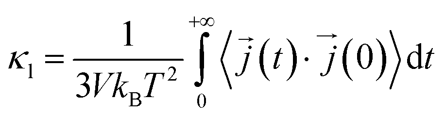 | (5) |
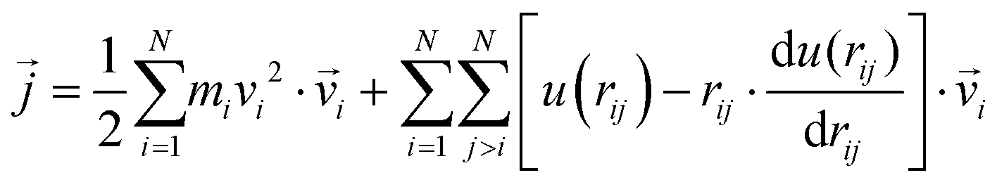
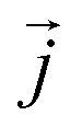 is the instantaneous microscopic heat current vector, defined by106
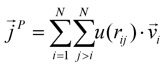
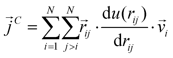
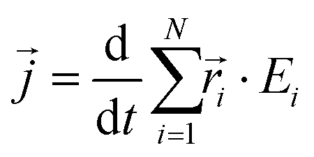 | (6) |
 is the position of atom i. For a pure body, the microscopic heat current
  is expressed as the sum of three fluctuations modes,
  ,
,  and
and  as107–109
 | (7) |
 | (8) |
 | (9) |
 | (10) |
 | (11) |
In a narrow sense, the third term emanates from the transfer of work done by the collision among the constituent atoms of the system.
Next, considering that in a computational simulation the time is not a continuous variable, in an MD the eqn (4) is discretized for Δt time steps as110,111
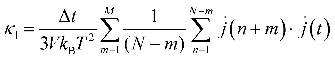 | (12) |
 is the heat current at the MD time step (n + m), N is the number of MD steps after the equilibration and M is the total number of steps over which the time average is calculated.
Acknowledgements
The authors thank the financial support from the Consejo Nacional deI Investigaciones en Ciencia y Tecnología (CONICET) through Grant PIP 11220200101385CO, FONCyT PICT-A-2020-2943, and the SeCyT-UNC Program PAGE#1. Computational resources were provided by the Centro de Cómputo de Alto Desempeño (CCAD-UNC), Universidad Nacional de Córdoba (https://ccad.unc.edu.ar/). M. B. C. thanks Fondecyt Regular Grant 1180023.References
- P. Keblinski, R. Prasher and J. Eapen, J. Nanopart. Res., 2008, 10, 1089–1097 CrossRef.
- H. Kang, Y. Zhang and M. Yang, Appl. Phys. A, 2011, 103, 1001–1008 CrossRef CAS.
- Y. Xuan and Q. Li, Int. J. Heat Fluid Flow, 2000, 21, 58–64 CrossRef CAS.
- K. V. Wong and O. De Leon, Adv. Mech. Eng., 2010, 2, 519659 CrossRef.
- S. R. Chitra and S. Sendhilnathan, Heat Transfer Asian Res., 2015, 44, 420–449 CrossRef.
- Y. Xuan and Q. Li, J. Heat Transfer, 2003, 125, 151–155 CrossRef CAS.
- S. Sarkar and R. Panneer Selvam, J. Appl. Phys., 2007, 102, 074302 CrossRef.
- S. Lee, S. U.-S. Choi, S. Li and J. A. Eastman, J. Heat Transfer, 1999, 121, 280–289 CrossRef CAS.
- J. Zhou, Z. Wu, Z. Zhang, W. Liu and Q. Xue, Tribol. Lett., 2000, 8, 213–218 CrossRef CAS.
- J. A. Eastman, S. U. S. Choi, S. Li, W. Yu and L. J. Thompson, Appl. Phys. Lett., 2001, 78, 718–720 CrossRef CAS.
- S. Bhanushali, N. N. Jason, P. Ghosh, A. Ganesh, G. P. Simon and W. Cheng, ACS Appl. Mater. Interfaces, 2017, 9, 18925–18935 CrossRef CAS PubMed.
- I. Khan, K. Saeed and I. Khan, Arabian J. Chem., 2019, 12, 908–931 CrossRef CAS.
- S. U. S. Choi, Z. G. Zhang, W. Yu, F. E. Lockwood and E. A. Grulke, Appl. Phys. Lett., 2001, 79, 2252–2254 CrossRef CAS.
- M.-S. Liu, M. C.-C. Lin, C. Y. Tsai and C.-C. Wang, Int. J. Heat Mass Transfer, 2006, 49, 3028–3033 CrossRef CAS.
- S. A. Angayarkanni and J. Philip, Adv. Colloid Interface Sci., 2015, 225, 146–176 CrossRef CAS PubMed.
- S. M. Mamand, Appl. Sci., 2021, 11, 1459 CrossRef CAS.
- R. K. Sahu, S. H. Somashekhar and P. V. Manivannan, Procedia Eng., 2013, 64, 946–955 CrossRef CAS.
- N. Jardón-Maximino, M. Pérez-Alvarez, R. Sierra-Ávila, C. A. Ávila-Orta, E. Jiménez-Regalado, A. M. Bello, P. González-Morones and G. Cadenas-Pliego, J. Nanomater., 2018, 2018, 1–8 CrossRef.
- J. Lv, M. Bai, W. Cui and X. Li, Nanoscale Res. Lett., 2011, 6, 200 CrossRef PubMed.
- K. Apmann, R. Fulmer, A. Soto and S. Vafaei, Materials, 2021, 14(5), 1291 CrossRef CAS.
- R. M. Tilaki, A. Iraji zad and S. M. Mahdavi, Appl. Phys. A, 2007, 88, 415–419 CrossRef CAS.
- M. B. Gawande, A. Goswami, F.-X. Felpin, T. Asefa, X. Huang, R. Silva, X. Zou, R. Zboril and R. S. Varma, Chem. Rev., 2016, 116, 3722–3811 CrossRef CAS PubMed.
- V. Abhinav, K. R. R. Venkata, P. S. Karthik and S. P. Singh, RSC Adv., 2015, 5, 63985–64030 RSC.
- G. Sánchez-Sanhueza, D. Fuentes-Rodríguez and H. Bello-Toledo, Int. J. Odontostomatology, 2016, 10, 547–554 CrossRef.
- M. I. Din and R. Rehan, Anal. Lett., 2017, 50, 50–62 CrossRef CAS.
- A. Tegenaw, G. A. Sorial, E. Sahle-Demessie and C. Han, Environ. Res., 2020, 187, 109700 CrossRef CAS PubMed.
- A. Kamyshny and S. Magdassi, Nanomaterials for 2D and 3D Printing, 2017, pp. 119–160 Search PubMed.
- W. Chang, P. Wang, Y. Zhao, C. Ren, B. N. Popov and C. Li, Surf. Coat. Technol., 2020, 398, 126077 CrossRef CAS.
- D. W. Boukhvalov, P. F. Bazylewski, A. I. Kukharenko, I. S. Zhidkov, Y. S. Ponosov, E. Z. Kurmaev, S. O. Cholakh, Y. H. Lee and G. S. Chang, Appl. Surf. Sci., 2017, 426, 1167–1172 CrossRef CAS.
- P. L. Ríos, P. Povea, C. Cerda-Cavieres, J. L. Arroyo, C. Morales-Verdejo, G. Abarca and M. B. Camarada, RSC Adv., 2019, 9, 8480–8489 RSC.
- J. Kwak, Y. Jo, S.-D. Park, N. Y. Kim, S.-Y. Kim, H.-J. Shin, Z. Lee, S. Y. Kim and S.-Y. Kwon, Nat. Commun., 2017, 8 Search PubMed.
- M. Scardamaglia, C. Struzzi, A. Zakharov, N. Reckinger, P. Zeller, M. Amati and L. Gregoratti, ACS Appl. Mater. Interfaces, 2019, 11, 29448–29457 CrossRef CAS PubMed.
- H. C. Lee, M. Jo, H. Lim, M. S. Yoo, E. Lee, N. N. Nguyen, S. Y. Han and K. Cho, Carbon, 2019, 149, 656–663 CrossRef CAS.
- H. Li, W. Kang, B. Xi, Y. Yan, H. Bi, Y. Zhu and Y. Qian, Carbon, 2010, 48, 464–469 CrossRef CAS.
- J. Wang, L.-N. Guo, W.-M. Lin, J. Chen, S. Zhang, S. Chen, T.-T. Zhen and Y.-Y. Zhang, Carbon, 2019, 150, 551 Search PubMed.
- A. Navidfar and L. Trabzon, Polym. Compos., 2021, 42, 944–954 CrossRef CAS.
- H. M. Ali and W. Arshad, Int. J. Heat Mass Transfer, 2017, 106, 465–472 CrossRef CAS.
- T. Tharayil, L. G. Asirvatham, V. Ravindran and S. Wongwises, Int. J. Heat Mass Transfer, 2016, 93, 957–968 CrossRef CAS.
- W. Yu, H. Xie, X. Wang and X. Wang, Phys. Lett. A, 2011, 375, 1323–1328 CrossRef CAS.
- Y.-F. Li, F.-X. Dong, Y. Chen, X.-L. Zhang, L. Wang, Y.-G. Bi, Z.-N. Tian, Y.-F. Liu, J. Feng and H.-B. Sun, Sci. Rep., 2016, 6, 37190 CrossRef CAS PubMed.
- P. Q. Phan, S. Chae, P. Pornaroontham, Y. Muta, K. Kim, X. Wang and N. Saito, RSC Adv., 2020, 10, 36627–36635 RSC.
- W. Leng, H. Michael Barnes, Q. Yan, Z. Cai and J. Zhang, Mater. Lett., 2016, 185, 131–134 CrossRef CAS.
- M. Son, J. Jang, Y. Lee, J. Nam, J. Y. Hwang, I. S. Kim, B. H. Lee, M.-H. Ham and S.-S. Chee, npj 2D Mater. Appl., 2021, 5 Search PubMed.
- R. Mehta, S. Chugh and Z. Chen, Nano Lett., 2015, 15, 2024–2030 CrossRef CAS.
- X. Glad, J. Gorry, M. S. Cha and A. Hamdan, Sci. Rep., 2021, 11 Search PubMed.
- S. Wang, X. Huang, Y. He, H. Huang, Y. Wu, L. Hou, X. Liu, T. Yang, J. Zou and B. Huang, Carbon, 2012, 50, 2119–2125 CrossRef CAS.
- S. Lee, J. Hong, J. H. Koo, H. Lee, S. Lee, T. Choi, H. Jung, B. Koo, J. Park, H. Kim, Y.-W. Kim and T. Lee, ACS Appl. Mater. Interfaces, 2013, 5, 2432–2437 CrossRef CAS PubMed.
- C.-A. Tseng, C.-C. Chen, R. K. Ulaganathan, C.-P. Lee, H.-C. Chiang, C.-F. Chang and Y.-T. Chen, ACS Appl. Mater. Interfaces, 2017, 9, 25067–25072 CrossRef CAS PubMed.
- S. Chen, A. Zehri, Q. Wang, G. Yuan, X. Liu, N. Wang and J. Liu, ChemistryOpen, 2019, 8, 58–63 CrossRef CAS PubMed.
- J. W. Lee, S. W. Kim, Y. L. Cho, H. Y. Jeong, Y. I. Song and S. J. Suh, J. Nanosci. Nanotechnol., 2016, 16, 11286–11291 CrossRef CAS.
- N. A. Luechinger, E. K. Athanassiou and W. J. Stark, Nanotechnology, 2008, 19, 445201 CrossRef PubMed.
- D. Choi, Y. Pyo, S.-B. Jung, Y. Kim, E. H. Yoon and C. S. Lee, Mater. Trans., 2016, 57, 1177–1182 CrossRef CAS.
- S. Xu, B. Man, S. Jiang, J. Wang, J. Wei, S. Xu, H. Liu, S. Gao, H. Liu, Z. Li, H. Li and H. Qiu, ACS Appl. Mater. Interfaces, 2015, 7, 10977–10987 CrossRef CAS PubMed.
- A. H. Zehri, A. Hafid Zehri, A. Nylander, L. Ye and J. Liu, 2019 22nd European Microelectronics and Packaging Conference & Exhibition (EMPC), 2019.
- T. T. Loong and H. Salleh, IOP Conf. Ser.: Mater. Sci. Eng., 2017, 226, 012146 Search PubMed.
- A. Rapallo, J. A. Olmos-Asar, O. A. Oviedo, M. Ludueña, R. Ferrando and M. M. Mariscal, J. Phys. Chem. C, 2012, 116, 17210–17218 CrossRef CAS.
- A. Spitale, M. A. Perez, S. Mejía-Rosales, M. J. Yacamán and M. M. Mariscal, Phys. Chem. Chem. Phys., 2015, 17, 28060–28067 RSC.
- S. Jalili, C. Mochani, M. Akhavan and J. Schofield, Mol. Phys., 2012, 110, 267–276 CrossRef CAS.
- X. Xu, D. Yi, Z. Wang, J. Yu, Z. Zhang, R. Qiao, Z. Sun, Z. Hu, P. Gao, H. Peng, Z. Liu, D. Yu, E. Wang, Y. Jiang, F. Ding and K. Liu, Adv. Mater., 2017, 1702944 Search PubMed.
- D. W. Boukhvalov, E. Z. Kurmaev, E. Urbańczyk, G. Dercz, A. Stolarczyk, W. Simka, A. I. Kukharenko, I. S. Zhidkov, A. I. Slesarev, A. F. Zatsepin and S. O. Cholakh, Thin Solid Films, 2018, 665, 99–108 CrossRef CAS.
- Q. Yi, J. Xu, Y. Liu, D. Zhai, K. Zhou and D. Pan, Chem. Phys. Lett., 2017, 669, 192–195 CrossRef CAS.
- L. Zhang, Y. Zhu, W. Teng, T. Xia, Y. Rong, N. Li and H. Ma, Comput. Mater. Sci., 2017, 130, 10–15 CrossRef CAS.
- T. P. C. Klaver, S.-E. Zhu, M. H. F. Sluiter and G. C. A. Janssen, Carbon, 2015, 82, 538–547 CrossRef CAS.
- Q. Li, Y. Yu, Y. Liu, C. Liu and L. Lin, Materials, 2017, 10, 38 CrossRef.
- H. Loulijat, H. Zerradi, S. Mizani, E. M. Achhal, A. Dezairi and S. Ouaskit, J. Mol. Liq., 2015, 211, 695–704 CrossRef CAS.
- W. Cui, Z. Shen, J. Yang, S. Wu and M. Bai, RSC Adv., 2014, 4, 55580–55589 RSC.
- H. Loulijat, H. Zerradi, A. Dezairi, S. Ouaskit, S. Mizani and F. Rhayt, Adv. Powder Technol., 2015, 26, 180–187 CrossRef CAS.
- P. Giannozzi, S. Baroni, N. Bonini, M. Calandra, R. Car, C. Cavazzoni, D. Ceresoli, G. L. Chiarotti, M. Cococcioni, I. Dabo, A. Dal Corso, S. de Gironcoli, S. Fabris, G. Fratesi, R. Gebauer, U. Gerstmann, C. Gougoussis, A. Kokalj, M. Lazzeri, L. Martin-Samos, N. Marzari, F. Mauri, R. Mazzarello, S. Paolini, A. Pasquarello, L. Paulatto, C. Sbraccia, S. Scandolo, G. Sclauzero, A. P. Seitsonen, A. Smogunov, P. Umari and R. M. Wentzcovitch, J. Phys.: Condens. Matter, 2009, 21, 395502 CrossRef PubMed.
- K. Burke, J. Chem. Phys., 2012, 136, 150901 CrossRef PubMed.
- P. Lai, J. Chem. Phys., 1995, 103, 5742–5755 CrossRef CAS.
- K. F. Garrity, J. W. Bennett, K. M. Rabe and D. Vanderbilt, Comput. Mater. Sci., 2014, 81, 446–452 CrossRef CAS.
- S. Grimme, J. Antony, S. Ehrlich and H. Krieg, J. Chem. Phys., 2010, 132, 154104 CrossRef PubMed.
- J. Tesch, P. Leicht, F. Blumenschein, L. Gragnaniello, M. Fonin, L. E. Marsoner Steinkasserer, B. Paulus, E. Voloshina and Y. Dedkov, Sci. Rep., 2016, 6, 23439 CrossRef CAS PubMed.
- J. L. Elechiguerra, J. Reyes-Gasga and M. J. Yacaman, J. Mater. Chem., 2006, 16, 3906–3919 RSC.
- S. Chen, A. L. Moore, W. Cai, J. W. Suk, J. An, C. Mishra, C. Amos, C. W. Magnuson, J. Kang, L. Shi and R. S. Ruoff, ACS Nano, 2011, 5, 321–328 CrossRef CAS PubMed.
- M. Sang, J. Shin, K. Kim and K. J. Yu, Nanomaterials, 2019, 9, 374 CrossRef CAS PubMed.
- X. Gu and R. Yang, Annu. Rev. Heat Transfer, 2016, 19, 1–65 CrossRef CAS.
- S. Kumar, S. Sharma, V. Babar and U. Schwingenschlögl, J. Mater. Chem. A, 2017, 5, 20407–20411 RSC.
- T. Ma, P. Chakraborty, X. Guo, L. Cao and Y. Wang, Int. J. Thermophys., 2020, 41 Search PubMed.
- S. M. Foiles, M. I. Baskes and M. S. Daw, Phys. Rev. B: Condens. Matter Mater. Phys., 1986, 33, 7983–7991 CrossRef CAS PubMed.
- R. Fraenkel, D. Schweke, Y. Haas, F. Molnár, D. Horinek and B. Dick, J. Phys. Chem. A, 2000, 104, 3786–3791 CrossRef CAS.
- T. Akiner, E. Kocer, J. K. Mason and H. Erturk, Mater. Today Commun., 2019, 20, 100533 CrossRef CAS.
- S. J. Stuart, A. B. Tutein and J. A. Harrison, J. Chem. Phys., 2000, 112, 6472–6486 CrossRef CAS.
- S. Sarkar and R. P. Selvam, MRS Online Proceedings Library (OPL), 2007, 1022, 108 Search PubMed.
- R. P. Selvam and S. Sarkar, ASME/JSME 2007 Thermal Engineering Heat Transfer Summer Conference, 2009, vol. 2, pp. 293–301 Search PubMed.
- S. Zeroual, H. Loulijat, E. Achehal, P. Estellé, A. Hasnaoui and S. Ouaskit, J. Mol. Liq., 2018, 268, 490–496 CrossRef CAS.
- A. P. Thompson, H. M. Aktulga, R. Berger, D. S. Bolintineanu, W. M. Brown, P. S. Crozier, P. J. in’t Veld, A. Kohlmeyer, S. G. Moore, T. D. Nguyen, R. Shan, M. J. Stevens, J. Tranchida, C. Trott and S. J. Plimpton, Comput. Phys. Commun., 2022, 271, 108171 CrossRef CAS.
- B. T. Polyak, USSR Comput. Math. Math. Phys., 1969, 9, 94–112 CrossRef.
- A. Yabuki and N. Arriffin, Thin Solid Films, 2010, 518, 7033–7037 CrossRef CAS.
- F. Taherkhani and A. Fortunelli, New J. Chem., 2022, 46, 19213–19229 RSC.
- S. Sharma, P. Kumar and R. Chandra, J. Compos. Mater., 2017, 51, 3299–3313 CrossRef CAS.
- S. Lee, D. Park and D.-B. Kang, Bull. Korean Chem. Soc., 2003, 24, 178–182 CrossRef CAS.
- F. Müller-Plathe, J. Chem. Phys., 1997, 106, 6082–6085 CrossRef.
- E. M. Achhal, H. Jabraoui, S. Zeroual, H. Loulijat, A. Hasnaoui and S. Ouaskit, Adv. Powder Technol., 2018, 29, 2434–2439 CrossRef CAS.
- L. Paulatto, F. Mauri and M. Lazzeri, Phys. Rev. B: Condens. Matter Mater. Phys., 2013, 87 Search PubMed.
- H.-Y. Cao, Z.-X. Guo, H. Xiang and X.-G. Gong, Phys. Lett. A, 2012, 376, 525–528 CrossRef CAS.
- L. Abadlia, F. Gasser, K. Khalouk, M. Mayoufi and J. G. Gasser, Rev. Sci. Instrum., 2014, 85, 095121 CrossRef CAS PubMed.
- H.-J. Shin, S.-M. Yoon, W. M. Choi, S. Park, D. Lee, I. Y. Song, Y. S. Woo and J.-Y. Choi, Appl. Phys. Lett., 2013, 102, 163102 CrossRef.
- S. K. Jaćimovski, M. Bukurov, J. P. Šetrajčić and D. I. Raković, Superlattices Microstruct., 2015, 88, 330–337 CrossRef.
- A. A. Balandin, S. Ghosh, W. Bao, I. Calizo, D. Teweldebrhan, F. Miao and C. N. Lau, Nano Lett., 2008, 8, 902–907 CrossRef CAS PubMed.
- P. Keblinski, S. R. Phillpot, S. U. S. Choi and J. A. Eastman, Int. J. Heat Mass Transf., 2002, 45, 855–863 CrossRef CAS.
- J. Eapen, J. Li and S. Yip, Phys. Rev. Lett., 2007, 98, 028302 CrossRef PubMed.
- L. Zhang, L. Tian, A. Zhang, Y. Jing and P. Qu, Int. J. Thermophys., 2021, 42, 44 CrossRef CAS.
- R. Lenin, P. A. Joy and C. Bera, J. Mol. Liq., 2021, 338, 116929 CrossRef CAS.
- X. Cui, J. Wang and G. Xia, Nanoscale, 2021, 14, 99–107 RSC.
- D. A. McQuarrie, Statistical Mechanics, University Science Books, 2000 Search PubMed.
- F. Sofos, T. Karakasidis and A. Liakopoulos, Int. J. Heat Mass Transfer, 2009, 52, 735–743 CrossRef CAS.
- S. Stackhouse and L. Stixrude, Rev. Mineral. Geochem., 2010, 71, 253–269 CrossRef.
- P. K. Schelling, S. R. Phillpot and P. Keblinski, Phys. Rev. B: Condens. Matter Mater. Phys., 2002, 65 Search PubMed.
- M. H. Khadem and A. P. Wemhoff, Chem. Phys. Lett., 2013, 574, 78–82 CrossRef CAS.
- K. V. Tretiakov and S. Scandolo, J. Chem. Phys., 2004, 120, 3765–3769 CrossRef CAS PubMed.
Footnote |
| † Electronic supplementary information (ESI) available. See DOI: https://doi.org/10.1039/d3cp00064h |
| This journal is © the Owner Societies 2023 |