Description of conformational ensembles of disordered proteins by residue-local probabilities

Abstract

The study of proteins with intrinsically disordered regions (IDRs) has emerged as an active field of research due to their intriguing nature. Although IDRs lack a well-defined folded structure, they play important functional roles in cells, following biological mechanisms different from those of the traditional structured proteins. Consequently, it has been necessary to re-design experimental and theoretical methods in order to face the challenges introduced by the dynamic nature of IDRs. In this work, we present an accurate and cost-effective method to study the conformational dynamics of IDRs based on the use of residue-local probabilistic expressions that characterize the conformational ensembles obtained from finite-temperature molecular dynamics (MD) simulations. It is shown that the good performance and the high convergence rates achieved with our method are independent of the IDR lengths, since the method takes advantage of the major influence of the identity and conformation of the nearest residue neighbors on the amino-acid conformational preferences to evaluate the IDR conformational ensembles. This allows us to characterize the conformational space of IDRs using a reduced number of probabilities which can be obtained from comparatively short MD simulations or experimental databases. To exemplify the usefulness of our approach, we present an application to directly detect Molecular Recognition Features (MoRFs) in an IDR domain of the protein p53, and to follow the time evolution of the thermodynamic magnitudes of this system during its exploration of the conformational space.

---

1. Introduction

During the last twenty years, the study of proteins with intrinsically disordered regions (IDRs) has emerged as an active research field,^1–6 since they do not obey the well-established paradigm that links protein function with a well-defined and folded three-dimensional structure of the polypeptide chain encoded in its amino acid sequence. In contrast, IDRs dynamically explore their conformational space while remaining functional⁴ and they are prevalent in eukaryotic genomes³ so they should be properly considered as a new class of proteins with biological mechanisms different from traditional structured proteins. Consequently, it has been necessary to adapt and/or elaborate new experimental⁷ and theoretical^8,9 methods able to face the subtleties and challenges introduced by the IDRs.

In this work, we focus in particular on what can be considered the most fundamental feature of any protein, its spatial structure. While ordered proteins show a folding free energy landscape with a deep absolute minimum, as visualized by the folding funnel picture, IDRs populate many different local minima, each of them corresponding to particular molecular conformations separated by free energy barriers that can be overpassed at room temperature.⁸ Therefore, IDRs have to be modeled structurally as dynamic conformational ensembles.^7,10–12 In practice resolving those conformational ensembles from either experiment or simulations is a difficult task with plenty of uncertainties. Although the number of experimental observables is substantially smaller than the number of IDRs configurational degrees of freedom, different valuable methods^13,14 have been recently developed for IDR ensemble reconstruction from experimental observables providing estimates of the extent of the conformational heterogeneity. From the computational side, Molecular Dynamics (MD) simulations are limited by the huge computational effort required to guarantee the complete exploration of the molecular conformational space,¹² along with the characterization of the huge number of conformational states. The two principal approaches that have been followed to try to overcome this computational issue are enhanced sampling¹⁵ and dimensionality reduction methods.¹⁶ Despite their partial success in describing the conformational thermodynamics of IDRs^17–20 and their ability to reproduce different experimental observables,^11,21,22 these methods still have some limitations that prevent their general use for the description of the IDR functional mechanisms, such as the risk of loss of information and representativeness,¹⁶ or in the enhanced sampling approach, the difficulties in the selection of suitable collective variables.¹⁵ Moreover, although the use of experimental data has been proven to be essential to validate observables generated from computational approaches and force fields in IDR systems, extending their use to the validation of conformational ensembles is more difficult because multiple ensembles can match the same experimental results within error after averaging.^7,10–13,23 More recently a promising alternative approach has been proposed²⁴ based on the exhaustive sample of small IDP fragments in MD simulations that are subsequently assembled into full-length IDPs.

Alternative ways to generate conformational ensembles of IDRs based on databases of pair residue (ϕ,ψ) dihedral angles have been proposed.^25–29 The idea of using conformational preferences of each amino acid depending on the nearest neighbor residues to elaborate molecular conformational ensembles has already been explored in structured proteins,^30,31 but its application to IDRs is particularly promising since their disordered character should facilitate a probabilistic description. However, the inspection of these methods reveals that they use different and incompatible approximations to evaluate the molecular conformational populations of the IDR ensemble in terms of the conformational probabilities of each residue in the molecular chain (see a more detailed discussion in Sections 2.1 and 3.1). Moreover, the resulting ensembles were in principle successfully validated by the doubtful method of averaging and comparing with experimental data, as previously noted.

In this work, we use extensive Molecular Dynamics simulations to show how the molecular conformational ensembles can be properly described through probabilistic expressions by using conformational preferences of each residue depending on the identity and conformation of the nearest neighbor residues. It is also shown that the probabilities required to generate the IDR conformational ensembles can be obtained with reasonable accuracy from short MD simulations. This approach allows us to directly detect Molecular Recognition Features (MoRFs) and to follow the time evolution of the thermodynamic magnitudes of the system as it explores the conformational space.

2. Methods

2.1 Probabilistic ensembles

We consider a general peptide chain R₁R₂…R_N composed by N residues in which the ith residue can adopt N_Ci different conformations (C_i). A molecular conformation is specified by a given set of conformations of the residues (C₁C₂…C_N). We are interested in the probability of finding the peptide in a given molecular conformation (P_mol). In probability theory the chain rule allows us to write P_mol accurately in terms of conditional probabilities as follows:³²

P_mol(C₁…C_N; R₁…R_N) = P₁(C₁|C₂…C_N;R₁…R_N)·P₂(C₂|C₃…C_N; R₁…R_N)⋯P_N−1(C_N−1|C_N; R₁…R_N)·P_N(C_N|R₁…R_N) (1a)

=P₁(C₁|R₁…R_N)·P₂(C₂|C₁;R₁…R_N)⋯P_N−1(C_N−1|C₁…C_N−2; R₁…R_N)·P_N(C_N|C₁…C_N−1; R₁…R_N) (1b)

where P_i(C_i|C_i+1…C_N; R₁…R_N) is the probability of finding the ith residue in the conformational region C_i assuming that the residues to the right of it are in the conformations C_i+1…C_N. An equivalent definition applies for the probability of finding the ith residue conditioned to the conformations of the residues placed to the left side of it. Of course, the terms right and left are used assuming the usual convention of numbering the residues from the N-terminal extreme into the C-terminal end. We find it convenient to explicitly indicate that the probabilities included in eqn (1a) and (1b) depend on the particular molecule considered.

While eqn (1a) and (1b) are equivalent and precise, they are not of practical use as they require knowledge of the conformational probability of any residue on the conformations of the remaining residues in the chain, no matter how far apart they are and, more importantly, they have to be evaluated for each molecule studied. However, eqn (1a) and (1b) are adequate starting points to introduce different approximations leading to probabilistic expressions that can provide reasonable and practical descriptions of the molecular conformational ensemble.

The simplest, and more drastic, approach is to assume that the conformational probability of any residue only depends on its identity and is independent of the identities and conformations of the remaining residues, that is

P_i(C_i|C_i+1…C_N; R₁…R_N) ⋍ P_i(C_i|R_i) (2)

P_i(C_i|C₁…C_i−1; R₁…R_N) ⋍ P_i(C_i|R_i) (3)

Substitution of these expressions into eqn (1a) or (1b) providesThis approximation is the so-called Flory's isolated-pair hypothesis, which is well-known^29,33–38 to provide a poor description of the molecular conformational ensemble, since interresidual interactions play an important role in the folding of a residue by modifying its accessible conformational space.

An improved approximation can be developed by assuming that the conformational probability of any residue depends on the identity of its nearest neighbor residues but not on their conformations. Thus, we write

P_i(C_i|C_i+1…C_N; R₁…R_N) ⋍ P_i(C_i|R_i−1R_iR_i+1) (5)

P_i(C_i|C₁…C_i−1; R₁…R_N) ⋍ P_i(C_i|R_i−1R_iR_i+1) (6)

and obtain the following expression for the molecular conformational probabilitiesP⁽¹⁾_mol establishes that the secondary structure of the peptide chain is the result of conformational preferences of amino acid triads,^34,39–54 instead of the isolated dynamic of each residue.

An even better approximation can be achieved by considering that the conformation of a given residue depends also on the conformation of its nearest neighbor residues

P_i(C_i|C_i+1…C_N; R₁…R_N) ⋍ P_i(C_i|C_i+1; R_i−1R_iR_i+1) (8)

P_i(C_i|C₁…C_i−1; R₁…R_N) ⋍ P_i(C_i|C_i−1; R_i−1R_iR_i+1) (9)

which leads to the expressionThe equivalence between eqn (10a) and (10b) is provided by the fundamental law of conditional probabilities P(A|B)P(B) = P(B|A)P(A).

The above procedure can be systematically extended by including the dependencies of the conformational preferences of residues on the identity and conformation of more distant residues. Formally, the resulting molecular conformational probabilities will be closer to the accurate result of eqn (1a) and (1b) in each step. However, the more dependencies that are included in the probability expressions, the more questionable their practical use will be since the conditional probabilities have to be calculated from limited sets of data provided by MD simulations or structure-encoding coil databases.²⁹ Each time an additional dependency is included, the available data needed for the calculation of the conditional probabilities are further fractionated compromising their accuracy. Nevertheless, P⁽¹⁾_mol and P⁽²⁾_mol provide good descriptions of the molecular conformational ensemble of peptides with IDRs as shown below.

We note that previous works^29,30 have proposed the use of probability terms depending simultaneously on the conformations of both nearest neighbor residues, that is P_i(C_i|C_i−1C_i+1, R_i−1R_iR_i+1), to build conformational ensembles of IDRs. These kinds of terms are absent in P⁽⁰⁾_mol and P⁽²⁾_mol because of the structure of the original accurate probabilistic expression given in eqn (1) where the individual probabilities of every residue only depend on the conformations of its neighbors placed on its left or right side.

In addition, some works have proposed the use of probability terms based on dimers.^28,30,31 In particular Cukier²⁸ has proposed evaluating the molecular conformational probabilities through the following expression

where it is certainly assumed that the conformational probabilities of a residue depends on the identity of the nearest neighbor residue placed to the left, but is completely independent on the right-side residue identity. Therefore, Cukier's equation differs from eqn (7) where the dependence on the identity of both nearest neighbour residues is taken into account. Although this contradicts the experimental findings³⁰ that the conformational preferences of a residue depend on the identity of its two nearest neighbor residues, we discuss this issue in our numerical tests for the sake of completeness.

2.2 MD simulations

MD simulations of peptides with sequences taken from the C-terminal (CT) and the proline rich (PR) IDR domains of p53⁵⁵ were carried out in order to test the reliability of the molecular conformational ensembles provided by the different approximations described in the previous section (see Table 1). Since the number of molecular conformations increases quickly with the number of residues, a first set of calculations was performed with peptides including only six residues for which the converged results could be extracted for the molecular conformational populations. These six-residue peptides are heterogeneous in their sequences, thus providing a good test set. Additionally, two peptides with 20 residues were included in our study. They have been chosen for their different characters. Peptide 20a is heterogeneous in its sequence while peptide 20b is rich in proline and alanine, so that similar amino acid triads appear along its chain allowing us to directly test some of the approaches proposed.

Table 1 Peptides analyzed in the present work

Label	Sequence^a	p53 domain	Residue numbers	N conf.
a All peptides were blocked using acetyl and N-methyl groups. b Number of molecular conformations.
6a	AHSSHL	CT	364–369	729
6b	KSKKGQ	CT	370–375	729
6c	STSRHK	CT	376–381	729
6d	KLMFKT	CT	382–387	729
6e	EGPDSD	CT	388–393	486
20a	AHSSHLKSKKGQSTSRHKKL	CT	364–383	∼3.5 × 10^9
20b	RVAPAPAAPTPAAPAPAPSW	PR	72–91	∼2 × 10^8

---

MD simulations were carried out with the molecules dissolved in water using the GROMACS package v2021.2.^56,57 Each solute molecule was surrounded by a number of water molecules ranging from 1400 to 12 000 (depending on the length of the peptide) and placed in a cubic box of a size chosen to reproduce the experimental density of the liquid at room temperature. All the molecules were described using the CHARMM36m⁵⁸ force field and the flexible TIP3P model was used for the solvent water molecules. This force field has been shown^59,60 to provide a good representation of proteins with IDRs. In any case the conformational preferences of the nearest neighbor residues are driven by geometric and steric constraints which are taken into account in all of the force fields commonly used to describe IDRs so that the main conclusions of this work are not compromised by the choice of the force field. Periodic boundary conditions were imposed in the simulations using the Particle–Mesh Ewald method to treat the long-range electrostatic interactions. The equations of motion were integrated using a time step of 0.5 fs. All simulations were carried out in a NVT ensemble at 298 K by coupling to a thermal bath.

Every system was equilibrated following a two-step process. In the first step, the system was propagated during 2 ns at 500 K to allow an extensive exploration of the molecular conformational space. In the second step, the system was equilibrated at 298 K over 5 ns. This procedure was repeated 300 times for every molecule. Each of these 300 initial configurations were propagated during 10 ns generating the same number of trajectories. During these production runs, the values of the dihedral angles were written every 5 fs. This computational strategy based on the use of many different starting conformations in short runs instead of a single starting structure in a long run²⁴ allowed us to obtain thermally and conformationally equilibrated systems for the six-residue peptides as tested by the convergence study of the conformational ensembles (see Section 3). In the case of the 20aa peptides, we performed further analysis of the conformational distribution of the starting structures by evaluating the end-to-end distance and the radius of gyration (see Fig. S1, ESI†). The statistical distribution of these collective variables confirms that the conformational ensemble of the starting structures is broadly distributed. We should note that even if some conformations at 500 K might not be representative of the room temperature ensemble, the lack of kinetic traps in IDRs due to their dynamic nature guarantees a fast transition towards room temperature conformations during the second equilibration step.

2.3 Conformational regions

In order to keep the number of molecular conformations tractable we follow Estaña et al.⁶¹ and simplify the structural classification of the conformational space of each residue by dividing it into three regions H, E and γ according to the values of the dihedral angles (ϕ,ψ). The only exceptions were glycine and proline that show characteristic behaviours.⁶² In the case of glycine, three different conformational regions were considered but different from the other residues and only two for proline. Details of the definition of the conformational regions are given in Fig. 1 and Table S1 (ESI†).

Fig. 1 Definition of the conformational regions in the Ramachandran plot for residues (a) glycine, (b) proline, and (c) all others. Region γ comprises all the remaining dihedral angle values excluded by the previously defined regions. Region H (helical) includes α_R and α' conformations. Region E (extended) includes pPII and β conformations. Probabilities have been calculated by dividing the (ϕ,ψ) conformational space into a 1° × 1° grid.

2.4 Comparison between ensembles

A conformational ensemble is characterized by the values of the probabilities of each molecular conformation , where [Doublestruck C]_j = (C₁C₂…C_N) is a given molecular conformation and N_conf is the total number of molecular conformations. In this work, we consider three different conformational ensembles. The first one is simply obtained from the MD simulations by counting how many times a given molecular conformation appears and it is represented as {P^sim_mol([Doublestruck C]_j)}. The probabilistic ensembles {P⁽¹⁾_mol([Doublestruck C]_j)} and {P⁽²⁾_mol([Doublestruck C]_j)} are generated using eqn (7) and (10a) and (10b) respectively, where the probabilities for each residue are again evaluated from the MD simulation data by counting. Let us recall that we use in this paper the terms probability and population of a molecular conformation as equivalent, with the only difference being that the probabilities are normalized and the populations are given in percentages.

In order to measure the similarity between two conformational ensembles {P_mol} and {} we use different scores.⁶³ The simplest one is the Pearson correlation coefficient (PCC or r) using x_j = P_mol([Doublestruck C]_j} and y_j = ([Doublestruck C]_j} as variables. However, the use of PCC may be compromised when the set of values include results of very different magnitude, as is the case for the conformational populations, leading us to underestimate the contribution of the smallest values. Therefore, we also include the Jensen–Shannon divergence⁶³ (JSD) a symmetrized and smoothed version of the Kullback–Leibler divergence (KLD) given by

whereJSD is well-defined even when one molecular probability is zero in one ensemble and nonzero in the other.

In order to evaluate the performance of the probabilistic conformational ensembles {P⁽¹⁾_mol([Doublestruck C]_j)} and {P⁽²⁾_mol([Doublestruck C]_j)} to reproduce the results of the simulations {P^sim_mol([Doublestruck C]_j)} two studies are required. Firstly, we need to establish the degree of convergence of any conformational ensemble with respect to the accumulated time of the trajectories used to calculate it. For instance, let us assume that we have run a total of 300 trajectories and want to measure the reliability of the conformational ensembles obtained by using only 5 trajectories. We divide the 300 trajectories in 60 groups of 5 trajectories and evaluate the average similarity score (PCC or JSD) by taking a high enough number of couples of groups (for instance 1–2, 3–4, 4–5, …,59–60). By considering groups of increasing size, we can fix the accumulated time required for a given conformational ensemble to be converged. Thus we established that a total of 3 μs of accumulated time is required to reach convergence in the {P^sim_mol([Doublestruck C]_j)} conformational ensembles of the molecules with 6 residues.

Secondly, we need to evaluate the ability of the probabilistic conformational ensembles calculated using only a fraction of the total accumulated time, to reproduce the converged {P^sim_mol([Doublestruck C]_j)} results. We will follow a similar procedure to that described above by dividing the trajectories into groups and evaluating the average similarity score between each group and the converged {P^sim_mol([Doublestruck C]_j)} results. By considering groups of increasing size, we determine the accumulated time required to obtain {P⁽¹⁾_mol([Doublestruck C]_j)} and {P⁽²⁾_mol([Doublestruck C]_j)} ensembles in agreement with the {P^sim_mol([Doublestruck C]_j)} converged results.

In the case of the polypeptides with 20 residues, it is computationally impossible to reach convergence in the {P^sim_mol([Doublestruck C]_j)} conformational ensembles due to the huge number of different molecular conformations. We then adopt a strategy based on considering all of the hexads of consecutive residues present in the molecule (1–6, 2–7,…, 14–19, 15–20). The convergence tests previously described are applied to each hexad and the average value of their similarity scores are considered as a measure of the resemblance between conformational ensembles. We note that this analysis is related to the hierarchical chain-growth approach recently proposed^24,64 in which the full-length molecule is split into overlapping fragments which can be sampled extremely in MD simulations.

Overall, our analysis revealed that the use of JSD or PCC scores did not alter at all the trends and conclusions. Accordingly, we carry out the convergence analysis using the JSD scores and use the PCC score to describe the representativity of the probabilistic conformational ensembles.

3 Results and discussion

3.1 First insights into the influence of neighbor residues

The particular amino acid sequence of the N-terminal p53 (p53-PR) domain, rich in proline (Pro) and alanine (Ala) residues, gives us the opportunity to explore the potential influence of the neighbor residues in the conformational population of IDR amino acids. The evaluation of seven Pro, four of them in APA triads and three of them changing one of the Ala neighbors by Serine (Ser) or Threonine (Thr) were selected for the analysis (see Fig. 2a). The conformational ensemble of p53-PR residues was obtained from MD simulations (see Methods 2.2) and the populations of the different conformational regions for Pro were evaluated. The results in Fig. 2a first indicate that Pro residues in the APA triads have similar conformational populations. In addition, changing the right Ala neighbor by Ser barely modifies the conformational ensemble of Pro. However, including a Thr as a neighbor, either on the left or right side, significantly modifies the conformational ensemble populations of Pro.

Fig. 2 Conformational probabilities of proline and alanine residues that have one or two similar neighbour residues in the N-terminal disordered region of p53 (72–91). (a) Population of the conformational regions of 7 different Pro residues and 2 different Ala residues. (b) Jensen–Shannon divergence evaluation between the Ramachandran diagrams of the seven Pro residues. (c) Conformational Ramachandran maps of Pro in AP⁷⁷A and AP⁸⁰T triads. Inset: Graphical representation of the p53-PR region.

The conformational ensembles of two Ala residues in PAA triads (see Fig. 2a) were also analyzed, and it was found that they have a similar population distribution. Regretfully, other Ala residues in the p53-PR domain that have Pro as a right neighbor, such as PAP, AAP, or VAP triads, are not suitable for comparison, since residues preceding Pro have a particularly restricted Ramachandran plot.⁶²

The 364–383 sequence of the C-terminal p53 domain (p53-CT) has two additional examples of residues with similar neighbors: (i) two Lysine (Lys) residues in the SK³⁷²K and HK³⁸¹K triads having both Lys on the right and Ser or Histidine (His) on the left, and (ii) two Ser residues in the HS³⁶⁶S and SS³⁶⁷H triads that swap the neighboring Ser and His on the left and right side. A similar evaluation of the conformational probabilities shows that these differences in the neighbor identities or their left/right position significantly modify the population distribution in these residues (see Fig. S2a and b, ESI†). Moreover, the population distribution of Ser in the HS³⁶⁶S triads was evaluated for different neighbor conformations on the right and left sides, just to confirm their influence (see Fig. S2c, ESI†), as already noted in previous studies.²⁹

In order to avoid the selection of the conformational regions being a factor that influences the analysis, the full conformational Ramachandran diagrams of p53-PR prolines were evaluated and compared. Following the approach of previous works,^63,65 a Jensen–Shannon divergence test (see the Methods section) between the Ramachandran diagrams of each Pro couple was performed (see Fig. 2b) to measure the similarity between them. The higher divergence values that are obtained between Pro having Thr or Ala neighbors just confirm numerically the differences observed in the Ramachandran diagrams in Fig. 2c. The Ramachandran diagrams of the other p53-PR Pro are collected in Fig. S3 (ESI†).

Overall, this comparison analysis is a simple and straightforward way to visualize the influence of the identity and the conformation of the neighbor residues on the conformational distribution of a certain amino acid. To confirm the general statement that the identity of the amino acid triads rules the conformational ensemble of the central residue of the triad, the previous analysis should be obviously extended to all amino acid combinations. Nevertheless, we have indeed shown that the identity of neighbour residues, their position on the left/right side and their conformation may significantly affect the conformational populations of the central residue. Moreover, our results align with previous computational evidence that highlights the influence of the nature and conformation of the nearest neighbour residues in the conformation probability distribution of the central amino acid.^36–38 Accordingly, previous approaches that ignore, even partially, these considerations include a systematic error in the evaluation of the conformational populations.^28,30

3.2 Using short peptides for an accurate evaluation of the probabilistic conformational ensembles

The number of molecular conformations defined by all the possible combinations of residue conformations grows exponentially with the number of residues (see Table 1), and so do the computational cost required to generate by MD simulations converged {P^sim_mol([Doublestruck C]_j)} conformational ensembles that can be used as patterns to measure the quality of the approximate {P⁽¹⁾_mol([Doublestruck C]_j)} and {P⁽²⁾_mol([Doublestruck C]_j)} probabilistic ensembles. In practice, it is impossible to reach convergence in the populations of the molecular conformations of the polypeptide with 20 residues included in this study. Nevertheless, one can mitigate the computational cost by studying short peptides that still conserve their intrinsic disorder nature. Thus, the CT domain of p53 was split in 5 peptides of 6 amino acids in length and each of their conformational ensembles generated by MD was evaluated. To compare the performance of the approximations made in other peptides that preferentially populate a certain conformation, the 6-aa poly-Alanine peptide was also included in our study.

The region 376–381 of the p53-CT domain (see Fig. 3a) was selected as a representative example among all the analyzed peptides. The first analysis focuses on the convergence of the conformational ensembles obtained in the simulations and those derived from probabilistic expressions. This was evaluated by using the Jensen–Shannon divergence (JSD) protocol as proposed by Tiberti et al.⁶⁵ This descriptor shows how similar the probabilities ensembles are that are obtained from two different sets of trajectories at equal accumulated simulation times (see the Methods section 2.4 for a more detailed description). While the JSD scores have a difficult simple geometric interpretation, as previously indicated by Lindorff-Larsen et al.,⁶³ the analysis of the evolution of the JSD scores along the simulation until they achieve the lowest asymptotic value is a good convergence predictor. Fig. 3b shows that the conformational probabilities obtained from the {P⁽¹⁾_mol([Doublestruck C]_j)} and {P⁽²⁾_mol([Doublestruck C]_j)} probabilistic conformational ensembles achieve convergence at times of around 0.7–1 μs, while the JSD score from the {P^sim_mol([Doublestruck C]_j)} ensemble is still decreasing at 1.5 μs.

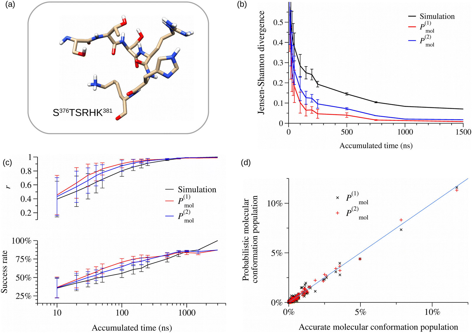Fig. 3 Comparison of different conformational probability evaluation methods in the region 376–381 of CT p53 domain. (a) Graphical representation of the 6-aa peptide S³⁷⁶TSRHK³⁸¹ of p53-CT. (b) Convergence evaluation of the conformational probabilities by computing the Jensen–Shannon divergence as a function of the accumulated time of the trajectories. (c) Accuracy evaluation of the probabilistic methods by using the Pearson coefficient (top) and the success rate of the most populated conformations accounting for the 75% of the total population of the peptide (bottom). (d) Comparison between the accurate conformational populations obtained from the simulations and those obtained from the approximate expressions P⁽¹⁾_mol and P⁽²⁾_mol.

The accuracy of the probabilistic methods was checked by employing the Pearson coefficient and the populations of the {P^sim_mol([Doublestruck C]_j)} conformational ensembles obtained from the 3 μs MD simulations were used as the reference. The results plotted in Fig. 3c show that at short simulation times, i.e. 100 ns, the probabilistic {P⁽¹⁾_mol([Doublestruck C]_j)} and {P⁽²⁾_mol([Doublestruck C]_j)} conformational ensembles give better predictions than those obtained with {P^sim_mol([Doublestruck C]_j)}. Only at longer times of 1 μs, do the {P^sim_mol([Doublestruck C]_j)} results outperform those obtained using the probabilistic expressions. It is noticeable that the convergence of the accuracy of the probabilistic conformational ensembles calculated using the probabilities in the P⁽¹⁾_mol and P⁽²⁾_mol expressions is faster than the results of the direct counting method ({P^sim_mol([Doublestruck C]_j)}) although they use the same set of data. It is also worth noticing that the results obtained with P⁽¹⁾_mol have a slightly better performance than the P⁽²⁾_mol ones before achieving simulation times of ∼500 ns. This is due to the fact that the number of probabilities by residue to be converged in the calculation of P⁽¹⁾_mol is substantially smaller than that of P⁽²⁾_mol due to the use in this last case of probabilities that depend on the conformation of the neighbor residues. At the temporal region of 1–1.5 μs, in which all conformational probabilities achieved convergence, the {P^sim_mol([Doublestruck C]_j)} results are obviously the most accurate. Nevertheless, the results obtained with both approximate expressions can be considered very good predictions, as shown by the Pearson correlation coefficient values close to 1 and the high success rates of prediction of above 85%. The JSD descriptor was additionally employed to evaluate the quality of the approximations, obtaining similar results (Fig. S4, ESI†). Moreover, a direct comparison between the conformational populations of the accurate {P^sim_mol([Doublestruck C]_j)} ensemble and the probabilistic ensembles at 3 μs (see Fig. 3d) confirms the linear correlation and the correct predictions of the most populated conformation ensembles. The same good performance has been obtained for the other peptide 6-aa stretches of CT-p53 (Fig. S5–S8, ESI†).

A similar conformational analysis performed with the Ala peptide (Fig. S9, ESI†) shows that the P⁽¹⁾_mol approach underestimates the values of the most populated conformation, which corresponds to the all-extended conformation, while the same population calculated using the P⁽²⁾_mol expression is correctly predicted. This can be explained by considering the cooperative effect along the poly-Ala peptide chain that favors the extended conformation of a residue if the neighbors are already in the extended conformation.⁶⁶ This effect may be characteristic of protein sequences that preferentially populate a certain structural conformation, such as the poly-Ala peptide. Considering then the influence of the neighbor conformations must be essential for an accurate prediction of the conformational probabilities, while for intrinsic disordered fragments, in which the distribution of conformational populations is substantially wider, the cooperative effect is minor and the P⁽¹⁾_mol probabilities are indeed a good approximation.

In a nutshell, short peptides from IDRs have allowed us to examine the performance of two probabilistic approximations by direct comparison with the accurate computational results. We consider that this is a more appropriate method to evaluate in detail the accuracy of probabilistic predictors than the comparison of different magnitudes (J couplings, RDCs, …) obtained as averaged data of the probabilistic ensembles with the experimental data. Indeed, the proposed probabilistic approximations could be applied with any other force fields and MD simulation approaches, as all of them use similar potential functions to evaluate the intra- and inter-molecular non-bonded interactions responsible of the conformational distribution of proteins. The use of the probabilistic approximated expressions P⁽¹⁾_mol and P⁽²⁾_mol to build the conformational ensembles using the data from MD simulations shows huge potential, since the computed probabilities achieve convergence at a high rate (even 100 ns could be enough) while maintaining accurate results.

3.3 Conformational probabilities of intrinsic disordered regions: CT and PR p53 domains

To study the performance of the probabilistic approaches in standard IDRs that contain tens of residues, MD simulations of the p53 IDRs proline-rich and C-Terminal regions were performed (see Table 1 and Fig. 4). Following the analysis protocol (see Section 2.4), a convergence study was first performed. The results in Fig. 4a and b clearly show that the conformational populations calculated directly from the simulations are far from achieving convergence at the considered simulation times. In contrast, populations obtained with the P⁽¹⁾_mol and P⁽²⁾_mol approximations are already converged within a few hundreds of nanoseconds. This result can be explained by considering the expressions P⁽¹⁾_mol and P⁽²⁾_mol in eqn (7) and (10a) and (10b), respectively, which are calculated as the product of the conformational probabilities of each residue conditioned by its first neighbors (either considering only their identity or both their identity and conformation). Thus, the convergence of the probabilistic conformational ensembles of the whole peptide is achieved in these approximations if the conformational probabilities of each residue are correctly converged, and the convergence of these probabilities by residue is basically independent of the peptide length. This result emphasizes a fundamental advantage of the use of the probabilistic ensembles, that is, molecular conformations which might not be present in the MD trajectories can be properly predicted.

Fig. 4 Comparison of the different conformational probability evaluation methods in the regions 72–91 (p53-PR) and 362–383 (p53-CT) of p53. Convergence evaluation of the conformational probabilities by computing the Jensen–Shannon divergence as a function of the accumulated time of the trajectories for (a) p53-PR and (b) p53-CT peptides. Accuracy evaluation of the probabilistic methods by using the Pearson coefficient for (c) p53-PR and (d) p53-CT peptides. Inset: Graphical representation of the p53 protein model obtained from AlphaFold⁶⁷ with regions p53-PR and p53-CT highlighted in yellow and cyan, respectively.

The lack of convergence of the P^sim_mol probabilities in the 20-aa peptides prevents the use of the direct comparison method to evaluate the prediction accuracy of the probabilistic approximations. We then used the protocol detailed in Section 2.4, in which the conformational populations of any 6-aa segment within the peptides p53-PR and p53-CT are evaluated and the analysis considers the convergence of the populations for these short segments. In that case, the comparison of the performance of the probabilistic approximations can be performed by considering the average of all 6-aa segments contained in the p53-PR and p53-CT domains. The Pearson coefficient values in Fig. 4c and d show that the approximations P⁽¹⁾_mol and P⁽²⁾_mol predict with a high accuracy the probabilities of the conformational population ensembles for both p53 IDRs. As for the previous results obtained for short peptides, high prediction accuracies are already achieved by the probabilistic approximations at simulation times of a few hundreds of nanoseconds. Moreover, the JSD descriptor was also employed for the comparison, obtaining the same conclusions (see Fig. S10, ESI†).

Although the comparison between the probabilistic methods of the population distributions of the whole 20-aa IDRs is unapproachable, as already discussed, the strategy of evaluating the accuracy in 6-aa stretches belonging the IDRs confirms the excellent performance of the P⁽¹⁾_mol and P⁽²⁾_mol approximations in IDRs. According to our results, IDRs residue neighbors farther away in sequence than the first neighbors have a lower influence on the conformation probability distribution of each residue. This seems reasonable, since long-range interactions between amino acids are intimately related with the folding stability of polypeptides,^68,69 and IDRs lack a well-defined folded structure. What makes IDRs difficult to study through direct analysis with MD simulations, at the same time facilitates their study through probabilistic conformational ensembles, thus opening the door to different applications.

3.4 Applications: MoRFs and free energy evaluation

It is discussed^61,70 that a possible mechanism of binding between IDRs adopting a certain secondary structure and their protein target could occur through Molecular Recognition Features (MoRFs). MoRFs are structural motifs transiently stable in solution that could already interact with the protein target, acting as nucleation sites for completing the IDR folding by inducing fit. The first application deals with the evaluation of the conformational probabilities of this type of structural signatures, as previously suggested by Estaña et al.⁶¹ For example, 11 residues of the 22a p53-CT domain folds into an alpha-helix secondary structure during the binding of S100B(ββ) dimer (PDB 1dt7, see Fig. 5a). The conformational probability of the MoRF composed by the 3-aa signature {ααα} from the 3-μs MD conformational ensemble was evaluated by using the P⁽²⁾_mol expression (see Fig. 5b). According to these results, the ααα-MoRF located in K³⁸²LM³⁸⁴ shows the highest probability value inside the α-helix region. Interestingly, other MoRFs at the N-terminal end also show high probability values, although their role in the binding mechanism should be thoroughly investigated. In short, this example shows the great advantage of employing the probability approximate expressions, since the relative low computational cost allows the exhaustive explorations of MoRFs (much more than in the simple example). The converged probability of each MoRF is therefore guaranteed, in contrast with standard evaluations, which require an extraordinary computational effort, as in the work of Fadda et al.⁷⁰

Fig. 5 Evaluation of MoRFs probabilities in p53-CT. (a) Graphical representation of the p53-CT domain (367–388) bound to the S100B(ββ) dimer (PDB 1dt7). (b) Probabilities of MoRFs {ααα} along the CT-p53 domain in the 3-μs trajectory.

The second application is related with the exploration of the conformational free energy surface of the IDRs. To do so, the conformational space of the peptide is evaluated in more detail, by defining a grid of size 10 × 10 in the dihedral angle Ramachandran map of each residue providing 360 × 360 microstates per residue. The probability of each molecular conformation is expressed in terms of the microstates of every residue using the expression of P⁽¹⁾_mol in eqn (7). Then, the free energy of each molecular conformation can be calculated as follows

In other words, the free energy of the peptide is expressed as the sum of the free energies of the microstates of each residue. As the dihedral angles of each residue evolve along the MD trajectory, they will visit the different cells in the Ramachandran grid and therefore, F⁽¹⁾_mol will evolve.

As an example, in Fig. 6a the time evolution of the molecular free energy of the domain p53-CT 382–393, expressed with respect to the molecular free energy average in all trajectories, is displayed. The evolution of F⁽¹⁾_mol goes through different local maxima and minima. If we define a conformational change in a residue as the dihedral angle transition between two broad conformational regions defined in Table 1, the different conformational changes along the trajectories can also be located (blue circles in Fig. 6a). Interestingly, we observed that the conformational changes occur mostly at high values of F⁽¹⁾_mol.

Fig. 6 Free energy analysis in the p53-CT region (382–393) evaluation in the conformational changes. (a) Evolution of the conformational free energy in the MD trajectory. Residue conformational changes are highlighted as blue circles. (b) Average values of the conformational change free energies in each residue. Conformational regions are defined according to Table 1.

To analyze quantitatively this behavior, we computed the average values of F⁽¹⁾_mol during all possible conformational changes that take place in each residue of the p53-CT domain. The results in Fig. 6b just confirm that the average values of the peptide free energy in the conformational transition of any residue are always higher than the free energy average value. The main contribution to each molecular free energy value corresponds to the residue that performs the conformational change, while the other contributions of the remaining amino acids are usually negligible (data available in the ESI†). Moreover, certain conformational changes are shown to be energetically more favored than others, depending on the residues and the type of conformational change.

4. Conclusions

In this work, we have shown that P⁽¹⁾_mol and P⁽²⁾_mol expressions describe properly the conformational ensembles of IDRs and that they can be extracted from reasonable short MD simulations. Indeed, one of the greatest advantages of the probabilistic expressions is that their convergence rates are independent of the IDR protein length, as they are calculated considering only the identity and conformation of the residue neighbours. Therefore, the gain in MD computational time of the proposed approach will grow with the length of the considered IDRs. Consequently, they can be used to evaluate the probabilities of molecular conformations that are rarely visited, namely rare events, without carrying out computationally expensive MD simulations. While our study is based on a coarse grain analysis of the conformational space of each residue in order to obtain converged molecular conformational ensembles the probabilistic expressions can be straightforwardly extended to a fine grain analysis providing a rigorous framework to build conformational ensembles from the data included in structure-encoding coil databases using previously developed methodologies.^29,71 The remarkably fast convergence and the good accuracy of the probabilistic conformational ensembles may allow us to explore thoroughly the mechanisms of binding of IDRs, as well as the impact of mutations in their functionality. As shown in recent works,^50,72 there is still room for improvement in the accuracy of most of current force fields to represent accurately the conformational populations of IDRs. Nevertheless, the improvement towards more realistic force fields for IDRs is a work-in-progress in the community.⁵⁹ Moreover, the results obtained in this work encourage future works to develop MD-based conformational ensemble libraries of amino acid triads, which will help to improve the performance of new machine learning predictors. The same approach should be equivalently useful for the study of the conformational ensembles of unfolded peptides and proteins.

Conflicts of interest

There are no conflicts to declare.

Acknowledgements

This work was partially supported by the Fundación Séneca under Project 20789/PI/18. We thank Prof. J. Cortés (LAAS-CNRS) for some helpful discussions and the computational assistance provided by J. F. Hidalgo of the Servicio de Infraestructuras TIC de ATICA. We thank Prof. Federico Fogolari (University of Udine, Italy) for his fruitful discussions.

References

1. V. Uversky, Introduction to intrinsically disordered proteins (IDPs), Chem. Rev., 2014, 114, 6557–6560.
2. V. Uversky, Intrinsically disordered proteins and their “Mysterious” (meta)physics, Front. Phys., 2019, 7, 10.
3. R. Van Der Lee, M. Buljan, B. Lang, R. Weatheritt, G. Daughdrill, A. Dunker, M. Fuxreiter, J. Gough, J. Gsponer and D. Jones, et al., Classification of intrinsically disordered regions and proteins, Chem. Rev., 2014, 114, 6589–6631.
4. P. Wright and H. Dyson, Intrinsically disordered proteins in cellular signalling and regulation, Nat. Rev. Mol. Cell Biol., 2015, 16, 18–29.
5. H. Dyson, Making Sense of Intrinsically Disordered Proteins, Biophys. J., 2016, 110, 1013–1016.
6. A. Dishman and B. Volkman, Unfolding the Mysteries of Protein Metamorphosis, ACS Chem. Biol., 2018, 13, 1438–1446.
7. N. Salvi, in Intrinsically disordered proteins: Dynamics, binding, and function, ed. N. Salvi, 2019, pp. 37–64.
8. S.-H. Chong and S. Ham, Folding Free Energy Landscape of Ordered and Intrinsically Disordered Proteins, Sci. Rep., 2019, 9, 14927.
9. P. Robustelli, S. Piana, D. Shaw and D. Shaw, Mechanism of Coupled Folding-upon-Binding of an Intrinsically Disordered Protein, J. Am. Chem. Soc., 2020, 142, 11092–11101.
10. D. Boehr, R. Nussinov and P. Wright, The role of dynamic conformational ensembles in biomolecular recognition, Nat. Chem. Biol., 2009, 5, 789–796 , cited By 1182.
11. J. Mittal, T. H. Yoo, G. Georgiou and T. M. Truskett, Structural Ensemble of an Intrinsically Disordered Polypeptide, J. Phys. Chem. B, 2013, 117, 118–124.
12. U. R. Shrestha, J. C. Smith and L. Petridis, Full structural ensembles of intrinsically disordered proteins from unbiased molecular dynamics simulations, Comm. Biol., 2021, 4, 243.
13. E. Ravera, L. Sgheri, G. Parigi and C. Luchinat, A critical assessment of methods to recover information from averaged data, Phys. Chem. Chem. Phys., 2016, 18, 5686–5701.
14. A. Carlon, L. Gigli, E. Ravera, G. Parigi, A. M. Gronenborn and C. Luchinat, Assessing Structural Preferences of Unstructured Protein Regions by NMR, Biophys. J., 2019, 117, 1948–1953.
15. G. Bussi and A. Laio, Using metadynamics to explore complex free-energy landscapes, Nat. Rev. Phys., 2020, 2, 200–212.
16. F. Sittel and G. Stock, Perspective: Identification of collective variables and metastable states of protein dynamics, J. Chem. Phys., 2018, 149, 150901.
17. T. N. Do, W.-Y. Choy and M. Karttunen, Accelerating the Conformational Sampling of Intrinsically Disordered Proteins, J. Chem. Theory Comput., 2014, 10, 5081–5094.
18. D. Granata, F. Baftizadeh, J. Habchi, C. Galvagnion, A. De Simone, C. Camilloni, A. Laio and M. Vendruscolo, The inverted free energy landscape of an intrinsically disordered peptide by simulations and experiments, Sci. Rep., 2015, 5, 15449.
19. O. Kukharenko, K. Sawade, J. Steuer and C. Peter, Using Dimensionality Reduction to Systematically Expand Conformational Sampling of Intrinsically Disordered Peptides, J. Chem. Theory Comput., 2016, 12, 4726–4734.
20. P. Herrera-Nieto, A. Pérez and G. De Fabritiis, Characterization of partially ordered states in the intrinsically disordered N-terminal domain of p53 using millisecond molecular dynamics simulations, Sci. Rep., 2020, 10, 12402.
21. F. Sziegat, R. Silvers, M. Haehnke, M. R. Jensen, M. Blackledge, J. Wirmer-Bartoschek and H. Schwalbe, Disentangling the Coil: Modulation of Conformational and Dynamic Properties by Site-Directed Mutation in the Non-Native State of Hen Egg White Lysozyme, Biochemistry, 2012, 51, 3361–3372.
22. M. R. Jensen, M. Zweckstetter, J.-R. Huang and M. Blackledge, Exploring Free-Energy Landscapes of Intrinsically Disordered Proteins at Atomic Resolution Using NMR Spectroscopy, Chem. Rev., 2014, 114, 6632–6660.
23. T. Lazar, E. Martinez-Perez, F. Quaglia, A. Hatos, L. B. Chemes, J. A. Iserte, N. A. Mendez, N. A. Garrone, T. E. Saldano and J. Marchetti, et al., PED in 2021: a major update of the protein ensemble database for intrinsically disordered proteins, Nucleic Acids Res., 2021, 49, D404–D411.
24. L. M. Pietrek, L. S. Stelzl and G. Hummer, Hierarchical Ensembles of Intrinsically Disordered Proteins at Atomic Resolution in Molecular Dynamics Simulations, J. Chem. Theor. Comp., 2020, 16, 725–737.
25. P. Bernado, C. Bertoncini, C. Griesinger, M. Zweckstetter and M. Blackledge, Defining long-range order and local disorder in native alpha-synuclein using residual dipolar couplings, JACS, 2005, 127, 17968–17969.
26. P. Bernado, L. Blanchard, P. Timmins, D. Marion, R. Ruigrok and M. Blackledge, A structural model for unfolded proteins from residual dipolar couplings and small-angle x-ray scattering, Proc. Natl. Acad. Sci. U. S. A., 2005, 102, 17002–17007.
27. F. Fogolari, A. Corazza, P. Viglino and G. Esposito, Fast structure similarity searches among protein models: efficient clustering of protein fragments, Algorithms Mol. Biol., 2012, 7, 16.
28. R. Cukier, I Generating Intrinsically Disordered Protein Conformational Ensembles from a Database of Ramachandran Space Pair Residue Probabilities Using a Markov Chain, J. Phys. Chem. B, 2018, 122, 9087–9101.
29. A. Estaña, N. Sibille, E. Delaforge, M. Vaisset, J. Cortés and P. Bernadó, Realistic Ensemble Models of Intrinsically Disordered Proteins Using a Structure-Encoding Coil Database, Structure, 2019, 27, 381–391.
30. D. Ting, G. Wang, M. Shapovalov, R. Mitra, M. I. Jordan and R. L. Dunbrack Jr, Neighbor-Dependent Ramachandran Probability Distributions of Amino Acids Developed from a Hierarchical Dirichlet Process Model, PLoS Comput. Biol., 2010, 6, 1–21.
31. A. Jha, A. Colubri, K. Freed and T. Sosnick, Statistical coil model of the unfolded state: Resolving the reconciliation problem, Proc. Natl. Acad. Sci. U. S. A., 2005, 102, 13099–13104.
32. D. Schum, The Evidential Foundations of Probabilistic Reasoning, Northwestern University Press, 1994.
33. R. Pappu, R. Srinivasan and G. Rose, The Flory isolated-pair hypothesis is not valid for polypeptide chains: Implications for protein folding, Proc. Natl. Acad. Sci. U. S. A., 2000, 97, 12565–12570.
34. M. Zaman, M. Shen, R. Berry, K. Freed and T. Sosnick, Investigations into sequence and conformational dependence of backbone entropy, inter-basin dynamics and the flory isolated-pair hypothesis for peptides, J. Mol. Biol., 2003, 331, 693–711.
35. M. R. Betancourt and J. Skolnick, Local Propensities and Statistical Potentials of Backbone Dihedral Angles in Proteins, J. Mol. Biol., 2004, 342, 635–649.
36. O. Keskin, D. Yuret, A. Gursoy, M. Turkay and B. Erman, Relationships between amino acid sequence and backbone torsion angle preferences, Proteins: Struct., Funct., Bioinf., 2004, 55, 992–998.
37. A. K. Jha, A. Colubri, M. H. Zaman, S. Koide, T. R. Sosnick and K. F. Freed, Helix, Sheet, and Polyproline II Frequencies and Strong Nearest Neighbor Effects in a Restricted Coil Library, Biochemistry, 2005, 44, 9691–9702.
38. I. E. Chemmama, P. P. Chapagain and B. S. Gerstman, Pairwise amino acid secondary structural propensities, Phys. Rev. E, 2015, 91, 042709.
39. C. Penkett, C. Redfield, I. Dodd, J. Hubbard, D. McBay, D. Mossakowska, R. Smith, C. Dobson and L. Smith, NMR analysis of main-chain conformational preferences in an unfolded fibronectin-binding protein, J. Mol. Bio., 1997, 274, 152–159.
40. K. Chen, Z. Liu, C. Zhou, Z. Shi and N. Kallenbach, Neighbor effect on PPII conformation in alanine peptides, JACS, 2005, 127, 10146–10147.
41. F. Avbelj and R. Baldwin, Limited Validity of Group Additivity for the Folding Energetics of the Peptide Group, Proteins, 2006, 63, 283–289.
42. A. Baruah, P. Rani and P. Biswas, Conformational Entropy of Intrinsically Disordered Proteins from Amino Acid Triads, Sci. Rep., 2015, 5, 11740.
43. S. E. Toal, N. Kubatova, C. Richter, V. Linhard, H. Schwalbe and R. Schweitzer-Stenner, Randomizing the Unfolded State of Peptides (and Proteins) by Nearest Neighbor Interactions between Unlike Residues, Chemistry AEJ, 2015, 21, 5173–5192.
44. R. Schweitzer-Stenner and S. E. Toal, Construction and comparison of the statistical coil states of unfolded and intrinsically disordered proteins from nearest-neighbor corrected conformational propensities of short peptides, Mol. Biosys., 2016, 12, 3294–3306.
45. A. Bastida, J. Zúũiga, A. Requena and J. Cerezo, Energetic Self-Folding Mechanism in alpha-Helices, J. Phys. Chem. B, 2019, 123, 8186–8194.
46. A. Bastida, J. Carmona-García, J. Zúũiga, A. Requena and J. Cerezo, Intraresidual Correlated Motions in Peptide Chains, J. Chem. Inf. Model., 2019, 59, 4524–4527.
47. J. González-Delgado, P. Bernadó, P. Neuvial and J. Cortés, Statistical proofs of the interdependence between nearest neighbor effects on polypeptide backbone conformations, J. Struct. Biol., 2022, 214, 107907.
48. F. Avbelj and R. Baldwin, Origin of the neighboring residue effect on peptide backbone conformation, Proc. Natl. Acad. Sci. U. S. A., 2004, 101, 10967–10972.
49. B. Milorey, H. Schwalbe, N. O'Neill and R. Schweitzer-Stenner, Repeating Aspartic Acid Residues Prefer Turn-like Conformations in the Unfolded State: Implications for Early Protein Folding, J. Phys. Chem. B, 2021, 125, 11392–11407.
50. B. Milorey, R. Schweitzer-Stenner, B. Andrews, H. Schwalbe and B. Urbanc, Short peptides as predictors for the structure of polyarginine sequences in disordered proteins, Biophys. J., 2021, 120, 662–676.
51. K. M. Saravanan and S. Selvaraj, Dihedral angle preferences of amino acid residues forming various non-local interactions in proteins, J. Biol. Phys., 2017, 43, 265–278.
52. H. Tran, X. Wang and R. Pappu, Reconciling observations of sequence-specific conformational propensities with the generic polymeric behavior of denatured proteins, Biochemistry, 2005, 44, 11369–11380.
53. M. Baxa, E. Haddadian, A. Jha, K. Freed and T. Sosnick, Context and Force Field Dependence of the Loss of Protein Backbone Entropy upon Folding Using Realistic Denatured and Native State Ensembles, JACS, 2012, 134, 15929–15936.
54. J. DeBartolo, A. Colubri, A. K. Jha, J. E. Fitzgerald, K. F. Freed and T. R. Sosnick, Mimicking the folding pathway to improve homology-free protein structure prediction, Proc. Natl. Acad. Sci. U. S. A., 2009, 106, 3734–3739.
55. O. Laptenko, D. R. Tong, J. Manfredi and C. Prives, The Tail That Wags the Dog: How the Disordered C-Terminal Domain Controls the Transcriptional Activities of the p53 Tumor-Suppressor Protein, Trends Biochem. Sci., 2016, 41, 1022–1034.
56. B. Hess, C. Kutzner, D. van der Spoel and E. Lindahl, GROMACS 4: Algorithms for Highly Efficient, Load-Balanced, and Scalable Molecular Simulation, J. Chem. Theor. Comp., 2008, 4, 435–447.
57. S. Pronk, S. Páll, R. Schulz, P. Larsson, P. Bjelkmar, R. Apostolov, M. R. Shirts, J. C. Smith, P. M. Kasson and D. van der Spoel, et al., GROMACS 4.5: A High-Throughput and Highly Parallel Open Source Molecular Simulation Toolkit, Bioinformatics, 2013, 29, 845–854.
58. J. Huang, S. Rauscher, G. Nawrocki, T. Ran, M. Feig, B. L. de Groot, H. Grubmueller and A. D. MacKerell Jr., CHARMM36m: an improved force field for folded and intrinsically disordered proteins, Nat. Methods, 2017, 14, 71–73.
59. J. Huang and A. D. MacKerell Jr., Force field development and simulations of intrinsically disordered proteins, Curr. Opin. Struct. Biol., 2018, 48, 40–48.
60. P. Robustelli, S. Piana and D. Shaw, Developing a molecular dynamics force field for both folded and disordered protein states, Proc. Natl. Acad. Sci. U. S. A., 2018, 115, E4758–E4766.
61. A. Estaña, A. Barozet, A. Mouhand, M. Vaisset, C. Zanon, P. Fauret, N. Sibille, P. Bernadó and J. Cortés, Predicting Secondary Structure Propensities in IDPs Using Simple Statistics from Three-Residue Fragments, J. Mol. Biol., 2020, 432, 5447–5459.
62. B. Ho and R. Brasseur, The Ramachandran plots of glycine and pre-proline, BMC Struct. Biol., 2005, 5, 14.
63. K. Lindorff-Larsen and J. Ferkinghoff-Borg, Similarity Measures for Protein Ensembles, PLoS One, 2009, 4, 1–13.
64. L. S. Stelzl, L. M. Pietrek, A. Holla, J. Oroz, M. Sikora, J. Koefinger, B. Schuler, M. Zweckstetter and G. Hummer, Global Structure of the Intrinsically Disordered Protein Tau Emerges from Its Local Structure, JACS AU, 2022, 2, 673–686.
65. M. Tiberti, E. Papaleo, T. Bengtsen, W. Boomsma and K. Lindorff-Larsen, ENCORE: Software for Quantitative Ensemble Comparison, PLoS Comput. Biol., 2015, 11, 1–16.
66. A. Bastida, J. Zúũiga, A. Requena, B. Miguel and J. Cerezo, On the Role of Entropy in the Stabilization of alpha-Helices, J. Chem. Inf. and Model, 2020, 60, 6523–6531.
67. J. Jumper, R. Evans, A. Pritzel, T. Green, M. Figurnov, O. Ronneberger, K. Tunyasuvunakool, R. Bates, A. Žídek and A. Potapenko, et al., Highly accurate protein structure prediction with AlphaFold, Nature, 2021, 596, 583–589.
68. N. Go and H. Taketomi, Respective roles of short- and long-range interactions in protein folding, Proc. Natl. Acad. Sci. U. S. A., 1978, 75, 559–563.
69. M. Gromiha and S. Selvaraj, Importance of long-range interactions in protein folding, Biophys. Chem., 1999, 77, 49–68.
70. E. Fadda and M. G. Nixon, The transient manifold structure of the p53 extreme C-terminal domain: insight into disorder, recognition, and binding promiscuity by molecular dynamics simulations, Phys. Chem. Chem. Phys., 2017, 19, 21287–21296.
71. Z. Harmat, D. Dudola and Z. Gaspari, DIPEND: An Open-Source Pipeline to Generate Ensembles of Disordered Segments Using Neighbor-Dependent Backbone Preferences, Biomolecules, 2021, 11, 1505.
72. B. Andrews, J. Guerra, R. Schweitzer-Stenner and B. Urbanc, Do molecular dynamics force fields accurately model Ramachandran distributions of amino acid residues in water?, Phys. Chem. Chem. Phys., 2022, 24, 3259–3279.

---

Footnote

† Electronic supplementary information (ESI) available: Free energy values during the conformational change in each residue of the p53-CT domain and the respective energetic contributions of each residue (XLSX). Supplementary tables: Definition of the conformational regions of the residues. Supplementary figures: population of the conformational regions of different residues in the p53-CT domain; conformational Ramachandran maps of different Pro residues in the p53-PR domain; Jensen–Shannon divergence evaluation of the probabilistic methods for 376–381 p53-CT peptides; comparison of the probabilistic methods in different peptides from the p53-CT domain and poly-Ala peptide; and Jensen–Shannon divergence evaluation of the probabilistic methods for p53-CT and p53-PR domains (PDF). See DOI: https://doi.org/10.1039/d2cp05970c

---