
 Open Access Article
 This Open Access Article is licensed under a
 Creative Commons Attribution 3.0 Unported Licence
Protein solutions close to liquid–liquid phase separation exhibit a universal osmotic equation of state and dynamical behavior
Jan
Hansen
 ,
Stefan U.
Egelhaaf
and
Florian
Platten
*
,
Stefan U.
Egelhaaf
and
Florian
Platten
*
Condensed Matter Physics Laboratory, Heinrich Heine University, Universitätsstraße 1, 40225 Düsseldorf, Germany. E-mail: florian.platten@hhu.de
First published on 26th December 2022
Abstract
Liquid–liquid phase separation (LLPS) of protein solutions is governed by highly complex protein–protein interactions. Nevertheless, it has been suggested that based on the extended law of corresponding states (ELCS), as proposed for colloids with short-range attractions, one can rationalize not only the thermodynamics, but also the structure and dynamics of such systems. This claim is systematically and comprehensively tested here by static and dynamic light scattering experiments. Spinodal lines, the isothermal osmotic compressibility κT and the relaxation rate of concentration fluctuations Γ are determined for protein solutions in the vicinity of LLPS. All these quantities are found to exhibit a corresponding-states behavior. This means that, for different solution conditions, these quantities are essentially the same if considered at similar reduced temperature or second virial coefficient. For moderately concentrated solutions, the volume fraction ϕ dependence of κT and Γ can be consistently described by Baxter's model of adhesive hard spheres. The off-critical, asymptotic T behavior of κT and Γ close to LLPS is consistent with the scaling laws predicted by mean-field theory. Thus, the present work aims at a comprehensive experimental test of the applicability of the ELCS to structural and dynamical properties of concentrated protein solutions.
1 Introduction
The interactions between protein molecules in solution, in general, comprise repulsive and attractive contributions. If short-range attractions prevail, protein condensation is favorable.1–6 If the attractions are strong, proteins are likely to form amorphous aggregates. If they are moderate, proteins are prone to crystallize or phase separate. Protein solutions can form two coexisting liquid phases, one depleted and one enriched in proteins; this process is called liquid–liquid phase separation (LLPS).7,8 It has recently attracted considerable attention due to its relevance in cell biology, medicine, pharmaceutical industry, and protein crystallography, as illustrated by the following examples. Membraneless organelles formed via LLPS in the cytosol represent a way of intracellular organization and can regulate biochemical reactions.9,10In vivo, LLPS can induce pathological protein aggregation, e.g., in the context of amyloid diseases, cataract and sickle-cell anemia.11–13 In biopharmaceuticals, LLPS is likely to increase solution viscosity and might raise immunogenicity.14,15 Hence, conditions favoring LLPS should be avoided in formulation development. However, X-ray crystallographers can exploit conditions close to LLPS, as they might favor the growth of high-quality crystals needed for diffraction experiments.16–19The protein–protein interactions that govern the phase separation processes are highly complex. They are determined by the specific amino acid composition of the proteins, their internal molecular organization, their overall molecular shape with a heterogeneous distribution of functionally different moieties on their surfaces as well as on the physicochemical solution conditions. It is therefore challenging to decipher a physical rationale of protein phase behavior and the underlying interactions.
Nevertheless, coarse-grained approaches inspired by soft-matter physics have been applied to the highly complex interactions between protein molecules and have proven helpful in understanding the observed phase behavior.6 For example, the DLVO theory has been applied to describe the effects of salts, solvents and pH on the interactions of protein solutions under conditions relevant for crystallization and LLPS.20–25 Colloid models have also been applied to describe the experimentally obtained structure factor of protein solutions.26–32
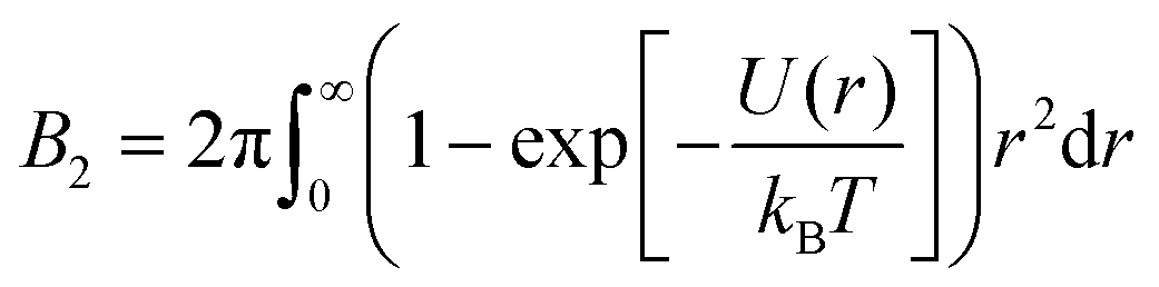
The state diagram of globular protein solutions exhibits striking similarities with the state diagram of colloids with short-range attractions, including a gas–crystal coexistence line below which a metastable gas–liquid binodal is submerged.6,33,34 With respect to LLPS of protein solutions, it would be appealing to adopt a colloid physics perspective and hence reduce the complexity of the situation. In this context, the application of the law of corresponding states (LCS) could provide a rationalization. It implies that simple fluids obey the same reduced equation of state.35 For monatomic systems, the LCS can be proven given pairwise additive and conformal interactions.36 As a consequence, many physical quantities, like the vapor pressure of the liquid or the Boyle point, fall onto a master curve when temperature and density are expressed relative to their values at the critical point, as demonstrated for some molecular systems.37 However, only few real substances can be described based on the original form of the LCS, but many fluids follow an extended form, the extended law of corresponding states (ELCS), which involves an additional parameter to describe the equation of state.38 For several systems with short-range attractions, molecular simulations suggest that the second virial coefficient at the critical temperature is fairly constant16 and that it can be used as an additional parameter to describe the equation of state.39 The second virial coefficient B2 can be considered as a measure of the strength and range of the interactions. For a spherosymmetric potential U(r) with center-to-center distance r, its definition reads
 | (1) |
Inspired by the ELCS as proposed for colloidal model systems, it has been found that also the LLPS binodals of protein solutions collapse onto a master curve if plotted in the b2vs. volume fraction ϕ plane and the repulsions of the different systems are alike or their differences are accounted for in terms of an effective σ.34,47–50 Nevertheless, despite the importance of LLPS and the possibility to rationalize the underlying interactions by the ELCS, systematic and comprehensive studies on the applicability of the ELCS to protein solutions are scarce, especially with respect to the structural and dynamical properties of concentrated solutions.
Here, the osmotic equation of state and the collective dynamics of protein solutions under conditions close to LLPS are systematically investigated. Static and dynamic light scattering experiments (SLS and DLS) are used to determine the isothermal osmotic compressibility κT and the relaxation rate of concentration fluctuations Γ, respectively. Lysozyme in brine is used as a model system for proteins with short-range attractions,51 whose strength can be modulated by additives.52 We thus exploit that, for this system, state diagrams (LLPS binodals) and interactions parameters (b2) have been reported previously.50 The spinodal lines, as inferred from SLS, as well as κT and Γ are found to exhibit a corresponding-states behavior. For moderately concentrated solutions, the ϕ dependence of κT and Γ can be consistently described by Baxter's model of adhesive hard spheres. The off-critical, asymptotic T behavior of κT and Γ close to LLPS is consistent with the scaling laws predicted by mean-field theory. Thus, the present work aims at a comprehensive experimental test of the applicability of the ELCS to structural and dynamical properties of concentrated protein solutions.
2 Experimental methods
2.1 Sample preparation
Purified, salt-free hen egg-white lysozyme powder (Worthington Biochemicals, cat. no. LS002933)), sodium chloride (NaCl; Fisher Chemicals), guanidine hydrochloride (GuHCl; Sigma, prod. no. G4505) and sodium acetate (NaAc; Merck, prod. no. 1.06268) were used without further purification.Ultrapure water with a minimum resistivity of 18 MΩ cm was used to prepare buffer and salt stock solutions. They were filtered several times meticulously (nylon membrane, pore size 0.2 m) in order to remove dust particles. The concentration of salt stock solutions, prepared in buffer, was determined from the excess refractive index. The protein powder was dissolved in a 50 mM NaAc buffer solution. The solution pH was adjusted to pH 4.5 by adding small amounts of hydrochloric acid. At this pH value, lysozyme carries a positive net charge Q = +11.4 e,53 where e is the elementary charge. Solutions with an initial protein concentration c ≈ 40–70 mg mL−1 were passed several times through an Acrodisc syringe filter with low protein binding (pore size 0.1 m; Pall, prod. no. 4611) in order to remove impurities and undissolved proteins. Then, the protein solution was concentrated by a factor of 4–7 using a stirred ultrafiltration cell (Amicon, Millipore, prod. no. 5121) with an Omega 10 k membrane disc filter (Pall, prod. no. OM010025). The retentate was used as concentrated protein stock solution. Its protein concentration was determined by UV absorption spectroscopy or refractometry.54 Protein concentrations c are related to the protein volume fraction ϕ = cvp, where vp = 0.740 mL g−1 is the specific volume of lysozyme, as inferred from densitometry.54 Sample preparation was performed at room temperature (21 ± 2) °C. Samples were prepared by mixing appropriate amounts of buffer, protein and salt stock solutions. Samples with cloud-points close to or above room temperature were slightly preheated to avoid (partial) phase separation upon mixing. Samples were analyzed or processed further (e.g., centrifuged) immediately after preparation in order to perform the measurements before crystallization sets in. In addition, equilibrium clusters55 are not expected to form as the repulsive interactions are largely screened.
2.2 Static light scattering (SLS) experiments
Light scattering experiments56 were performed with a 3D light scattering apparatus (LS Instruments AG) with a wavelength λ = 632.8 nm.Samples with 10 mg mL−1 ≤ c ≤ 160 mg mL−1 (0.007 ≤ ϕ ≤ 0.12) were investigated at selected temperatures 12.0 °C ≤ T ≤ 43.0 °C. As the samples are metastable with respect to crystallization, samples are analyzed directly after preparation. Samples investigated at different T were prepared separately. In order to minimize spurious effects of any residual dust or undissolved aggregates that were not removed by filtration, the samples were filled into thoroughly cleaned cylindrical glass cuvettes (diameter 10 mm) and centrifuged (Hettich Rotofix 32A) 30 min at typically 2500 g prior to the measurements. They were then very carefully placed into the temperature-controlled vat of the instrument filled with decalin.
The time-averaged scattered intensity was recorded. In order to check sample quality, also DLS experiments (see below) were performed on the same samples. Samples with indications of aggregates or dust particles were discarded. The meticulous filtration and centrifugation procedure was essential to obtain reproducible light scattering data. However, this protocol did not work for samples with c > 160 mg mL−1, possibly due to aggregation or crystallization.51,57
The absolute scattering intensity, i.e. the excess Rayleigh ratio R, varies with protein concentration c and temperature T. It was determined using toluene as a reference according to
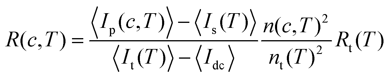 | (2) |
The refractive index of a sample solution, n, was measured with a temperature-controlled Abbe refractometer (Model 60L/R, Bellingham & Stanley) operated with a HeNe laser (λ = 632.8 nm) and at the temperature of the SLS experiment. Refractive index increments, dn/dc, were obtained from linear fits to the dependence of n on c.
In one-component solutions, the excess scattering typically contains information on the shape and size of the particles as well as the particle arrangement. Their contributions are reflected in the form factor P(Q) and the structure factor S(Q), respectively, where Q = (4πn/λ)sin(θ/2) is the magnitude of the scattering vector with the scattering angle θ. Then, the excess Rayleigh ratio R reads:
R(Q) = K![[thin space (1/6-em)]](https://www.rsc.org/images/entities/char_2009.gif) cMP(Q)S(Q) cMP(Q)S(Q) | (3) |
320 g mol−1 for lysozyme) and an optical constant K given by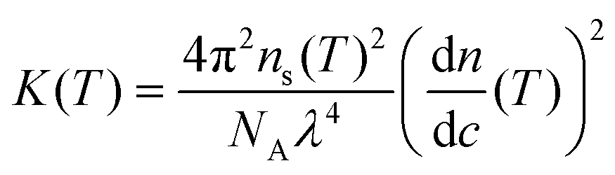 | (4) |
The effective protein diameter σ = 3.4 nm is small compared to λ, implying σQ ≪ 1. Nevertheless, for selected samples, experiments were performed at 30° ≤ θ ≤ 150° and R was indeed found to be independent of θ and hence of Q. In most of our experiments thus only one angle θ = 90° and hence Q ≈ 0.018 nm−1 was investigated. In addition to the DLS experiments, the independence of R on θ also suggested that large particles, such as impurities or aggregates, were absent.
Moreover, in the low-Q limit,
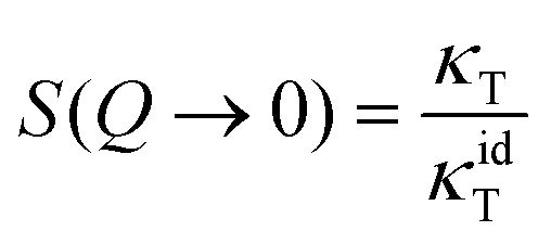 | (5) |
2.3 Dynamic light scattering (DLS) experiments
The samples investigated by SLS were also studied by DLS. In the vicinity of the LLPS spinodal or critical point, multiple scattering is expected to be important. In order to suppress these contributions, the 3D cross-correlation technique64 is applied here. The measured cross-correlation function g2(Δt) depends on lag time Δt and is defined as | (6) |
| g2(Δt) = B + β|f(Δt)|2 | (7) |
 | (8) |
 is a measure of the departure from a single exponential decay; here, in many cases
  and in some larger (typically 0.3). As the ISFs show a single-exponential decay and hence indicate diffusive behavior, the relaxation rate can be related to the collective diffusion coefficient Dc of the local concentration fluctuations via Γ = DcQ2.
2.4 Optical microscopy
For selected samples, the microscopic morphologies of the condensed protein states as well as the phase separation kinetics (nucleation, domain formation or coarsening) were monitored by conventional optical microscopy. Sample solutions were prepared at a temperature above the cloud-point, typically at 30 °C, and filled into a capillary.69 The capillary was mounted onto a home-built temperature-controlled microscope stage equipped with a thermoelectric cooler. The samples were quenched with about 0.5 K s−1 to specific temperatures and observed using an inverted brightfield microscope (Nikon Eclipse Ti-2) equipped with a 10× plan-fluor objective (Nikon) and a CMOS camera (Allied Vision, Mako U-130B, 512 × 512 px2) for at least 2 h. The pixel pitch was 0.485 μm px−1.3 Results and discussion
LLPS can occur when the protein–protein interactions are sufficiently attractive. Lysozyme in brine represents a model system dominated by short-range attractions and thus prone to crystallization or phase separation.51 The interactions can be tuned by additives.52 For this system, the LLPS binodals and the underlying protein–protein interactions in terms of b2 have been determined previously.50 The binodals are shifted by the additives (Fig. 1(A)), but they collapse onto a master curve if the temperature axis is replaced by the second virial coefficient (Fig. 1(B)).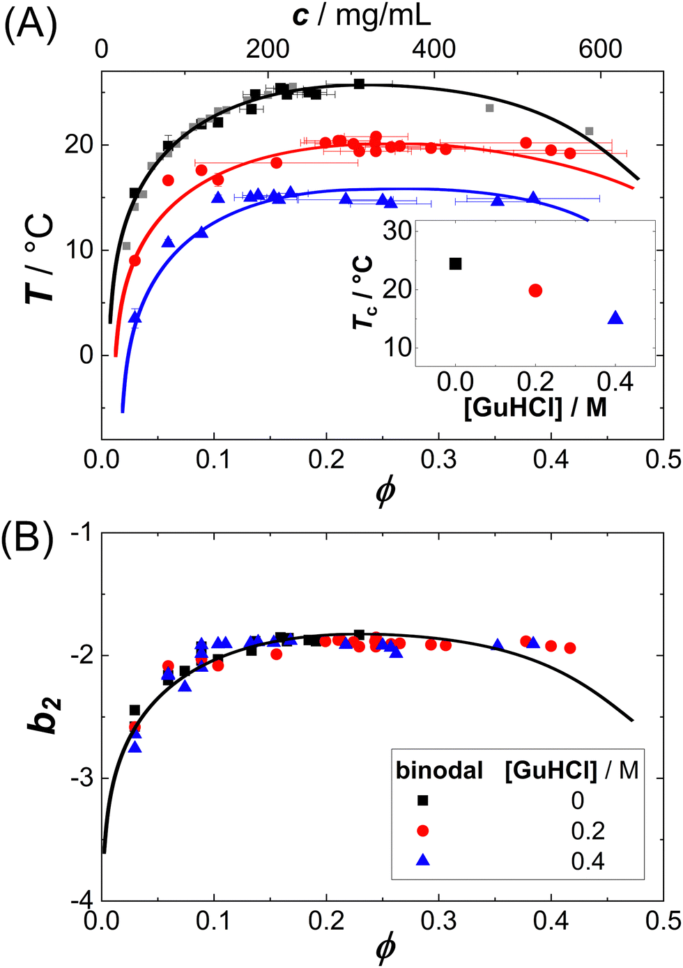 | ||
| Fig. 1 Liquid–liquid phase separation of protein solutions: (A) binodals of lysozyme solutions (pH 4.5, 0.9 M NaCl) in the temperature T vs. volume fraction ϕ (or protein concentration c) plane. Symbols denote different amounts of GuHCl, as specified in the legend. Lines are a guide to the eye. Inset: Critical temperature Tc for three different additive concentrations, which can be estimated based on a critical scaling ansatz, as detailed previously.7,8,25,34 (B) The same binodals as in (A), but in the normalized second virial coefficient b2vs. volume fraction ϕ plane. Data of (A) and (B) are replotted from ref. 50. | ||
In order to explore the applicability of the ELCS to static and dynamic properties of concentrated protein solutions, in the present work, this model system is investigated comprehensively by SLS and DLS experiments. The system is studied as a function of protein concentration, temperature and additive content in the vicinity of the LLPS binodal. However, an extremely close proximity as well as highly concentrated samples are avoided; therefore, it can be expected that simple, analytical models are applicable to the ϕ dependence of structural and dynamical data and mean-field values of the critical exponents describe the asymptotic T dependence of the data.
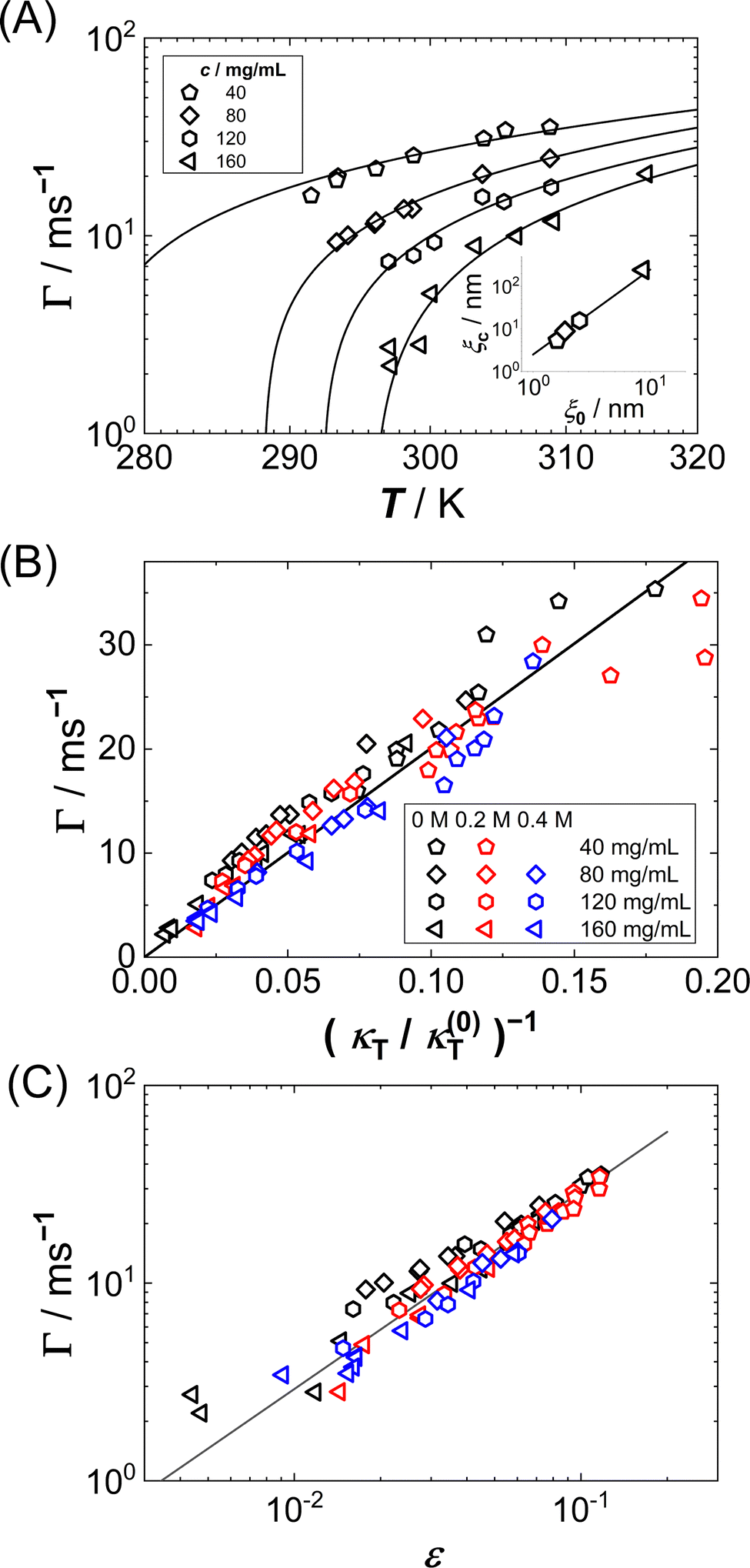
First, spinodal temperatures are inferred from the T dependence of the SLS data and added to the b2vs. ϕ plane (Fig. 1(A)). Then, the ϕ dependence of the isothermal compressibility κT is analyzed and a corresponding-states behavior is observed. Third, the relaxation rate Γ of the concentration fluctuations is determined and its T dependence is analyzed. Fourth, the ϕ dependence of the collective diffusion coefficient Dc is analyzed and a corresponding-states behavior is found.
3.1 Temperature dependence of the isothermal compressibility: corresponding-states behavior of the spinodal
The spinodal line is defined as the limit of thermodynamic stability. SLS has previously been used to determine the spinodal line of protein solutions.70–74 Upon approaching the spinodal by lowering T, κT is expected to increase according to an asymptotic power law behavior:| κT = κ0ε−γ | (9) |
 | (10) |
Fig. 2(A) shows exemplary data (symbols) of κT−1(T) for various protein concentrations c as indicated. As expected, the data can be described by linear fits (lines), yielding estimates of Ts as intercepts of the abscissa. Note that the spinodal line is submerged below the binodal and hence the κT−1(T) data have to be extrapolated by the fits. Moreover, at fixed T, κT−1(T) decreases with c, and hence larger intercepts of the abscissa and, correspondingly, Ts are observed, similar to the c dependence of the cloud-point temperatures shown in Fig. 1(A).
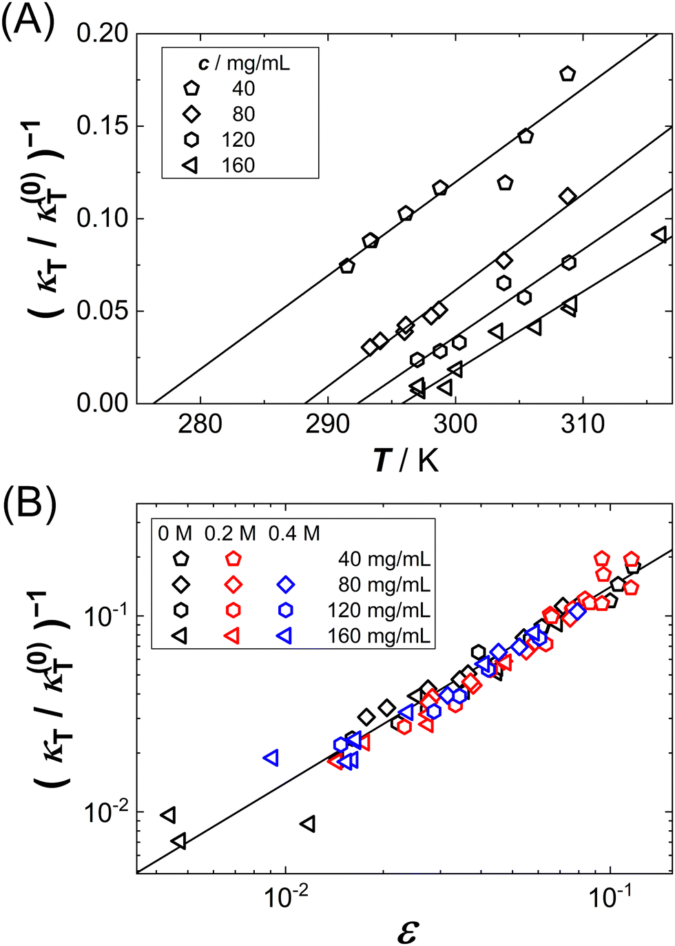 | ||
| Fig. 2 (A) Temperature T dependence of the inverse isothermal compressibility κT, normalized by κ(0)T = 1 (N m−2) (mg mL−1)−1, for different protein concentrations as indicated: experimental data (symbols) and linear fits (lines). (B) Dependence of the inverse isothermal compressibility κT, normalized by κ(0)T = 1 (N m−2) (mg mL−1)−1, on the reduced spinodal temperature ε = T/Ts − 1 where Ts is the spinodal temperature. Data (symbols), used to determine Ts shown in (A), i.e. for different GuHCl contents and protein concentrations (columns and rows in the legend, respectively). The solid line has a slope of 1. | ||
Fig. 2(B) shows all κT−1 data as a function of the reduced spinodal temperature ε together with a solid line of slope 1 on a double logarithmic representation. As expected from eqn (9), the different data sets collapse onto a single curve which shows a power-law behavior with the mean-field value γ = 1. The observed scaling behavior further supports the appropriateness of our approach to estimate Ts values. Eqn (9) was also fitted globally to the κT−1 data with a free, but global value of γ (not shown). This procedure yields γ = 0.97, further supporting the appropriateness of the mean-field value.
In addition to the data obtained in Fig. 2(A), similar experiments have been performed for the two other solution conditions (red circles and blue triangles in Fig. 1(A)). Fig. 3(A) shows the resulting Ts data (open symbols) and replots the binodals (full symbols). Indeed, for each of the three conditions, the spinodal is hidden below the binodal and thus also narrower than the binodal. With increasing ϕ, the spinodal approaches the binodal, as they are expected to coincide at the critical point. With increasing guanidine content, the spinodal shifts to lower T, similar to the decrease of the binodal. The inset shows the guanidine dependence of Ts for different protein concentrations together with a common linear fit. The slope of −26 K/M agrees with the previously observed value for the binodals.54 (For one particular solution condition, c = 40 mg mL−1 and 0.4 M GuHCl, the κT(T) are extrapolated over more than 30 K, resulting in a very low value of Ts with large uncertainty. This data point is omitted from further analysis.)
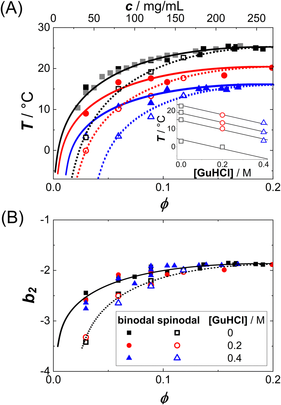 | ||
| Fig. 3 (A) Binodals (data as full symbols and guides to the eye as solid lines, replotted from Fig. 1, and spinodals (data (open symbols) and eye guides (dotted lines) of lysozyme solutions (0.9 M NaCl) with various amounts of GuHCl as in Fig. 1. Inset: Dependence of the spinodal temperatures on the guanidine concentration for different protein concentrations (increasing from bottom to top): data (open symbols) and global linear fits (lines). (B) The same binodals as in (A), but in the normalized second virial coefficient b2vs. volume fraction ϕ plane. Lines are guides to the eye. | ||
Since b2(T) data are available for our system (cf. circles in Fig. 5(B)),50 the spinodal lines of Fig. 3(A) can also be represented in the b2vs. ϕ plane. Fig. 3(B) shows both the binodal and spinodal lines in this representation. Again, similar to the binodals, the different spinodal lines collapse onto one another, indicating that the corresponding-states behavior previously observed for the binodals34,50 also holds for the spinodals.
Some solution conditions (marked by stars in Fig. 4(A)) have been examined by optical microscopy in order to study the phase separation kinetics in the metastable region between spinodal and binodal line as well as in the unstable region below the spinodal.
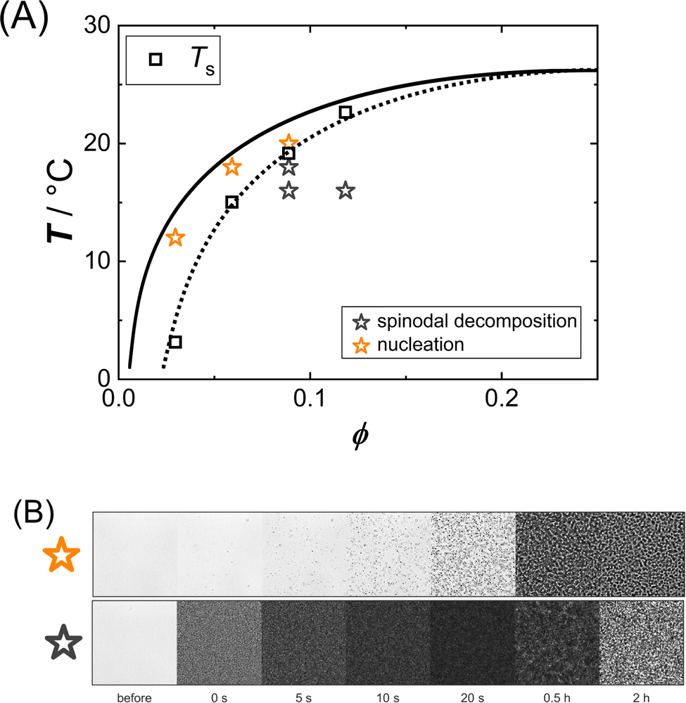 | ||
| Fig. 4 (A) Interpolated binodal (solid line), replotted from Fig. 1; spinodal temperatures (open squares) as inferred from the intercept of the abscissa in Fig. 2(A) connected by a dotted line as a guide to the eye; the solution conditions probed by optical microscopy are indicated by stars. (B) Optical micrographs (image size 248 × 248 μm2) illustrating the phase transition kinetics of samples phase separating via nucleation (top) and spinodal decomposition (bottom); in this case, ϕ = 0.06 (top) and ϕ = 0.09 (bottom) both at T = 18 °C, respectively. | ||
Exemplary time series of micrographs are shown in Fig. 4(B). In the metastable region, the microscopy data show the successive formation and growth of droplets, whereas in the unstable region the micrographs reveal a rapid initial darkening as the sample becomes turbid and at later stages the micrographs indicate domain formation and coarsening. The micrographs thus show qualitatively different phase separation kinetics depending on the location of the state. In the metastable region between binodal and spinodal, phase separation proceeds via droplet nucleation, while in the unstable region below the spinodal, spinodal decomposition is observed.
3.2 Volume fraction dependence of the isothermal compressibility: corresponding-states behavior of κT
Fig. 5(A) presents exemplarily data on the ϕ dependence of κT, normalized by the respective value of an ideal solution κ(id)T. This normalization corresponds to the low-Q limit of the static structure factor or to a normalized derivative of the osmotic pressure and is thus directly related to the osmotic equation of state (EOS). Data for different additive concentrations [GuHCl] and temperatures T, where the temperature is given relative to the critical temperature, T/Tc, and displayed as symbols in the same color. Remarkably, though obtained under different solution conditions (i.e., different guanidine concentrations and different absolute temperatures), normalized κT data cluster together on a single curve for a given T/Tc. This collapse indicates a universal osmotic EOS close to Tc and thus provides an experimental validation of the ELCS.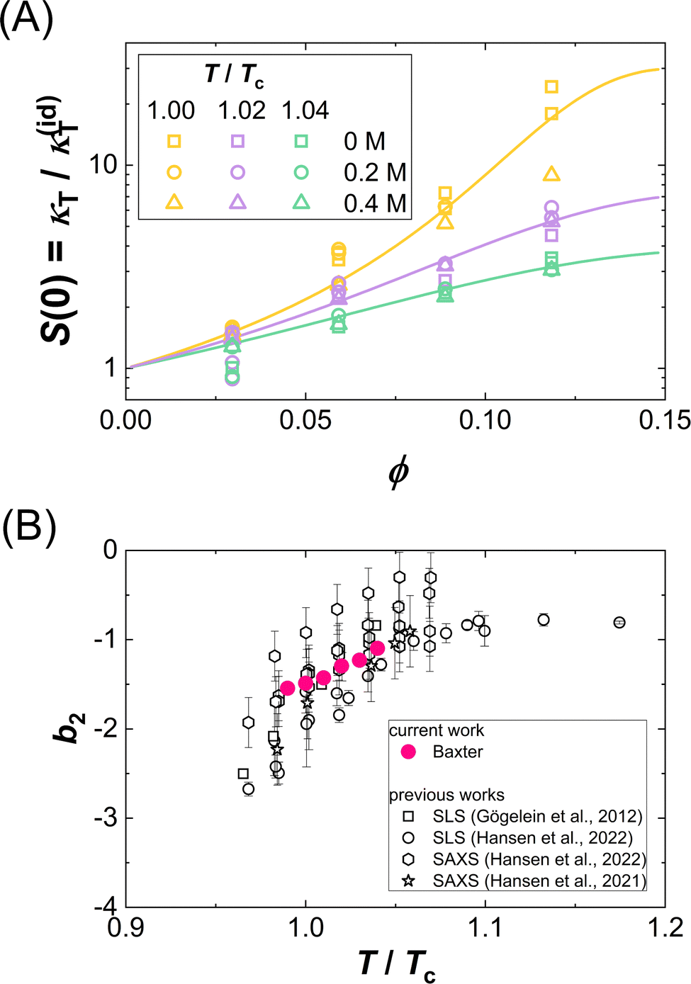 | ||
| Fig. 5 (A) Volume fraction ϕ dependence of the isothermal compressibility κT normalized by the isothermal compressibility κ(id)T of an ideal solution: Experimental data (symbols) for different temperatures normalized by the critical temperature, T/Tc, and guanidine concentrations are marked by symbol color and type, respectively. Lines are one-parameter fits to eqn (11). (B) Normalized second virial coefficient b2 as a function of the reduced temperature T/Tc: data retrieved from the fits in (A) and literature data23,25,50,82 are shown as full and open symbols, respectively. | ||
The ϕ dependence of the isothermal compressibility for low salt content,75i.e., far away from LLPS, has been successfully described by an analytical expression for the compressibility of the adhesive hard-sphere model in the Percus–Yevick approximation:76–81
 | (11) |
 | (12) |
 | (13) |
Fig. 5(B) shows the resulting values (full symbols), as retrieved from model fits to all κT data of the present work. The magnitude of b2 is found to increase with T/Tc, i.e., attractions are weakened for temperatures further away from the binodal. The value observed for T/Tc ≈ 1 is close to b2 = −1.5, as proposed by Vliegenthart and Lekkerkerker.16 Moreover, the figure contains literature data23,25,50,82 on b2(T/Tc) for the present system obtained by light scattering from dilute solutions and from the analysis of small-angle X-ray scattering experiments. The present data and the independent literature data agree with each other, supporting the significance of the obtained model parameter (τ) as well as the appropriateness of the model. Further support stems from independent SAXS measurements, whose Q dependent structure factor contribution was accurately described by approximate, analytical expression of the Baxter model.82
3.3 Temperature dependence of the relaxation rate of concentration fluctuations: off-critical slowing down correlated with divergence of the compressibility
In the preceding Sections 3.1 and 3.2, structural properties of protein solutions are analyzed, whereas dynamical properties are investigated in this and the following section. κT quantifies the amplitude of concentration fluctuations83 and shows an asymptotic power-law behavior when T becomes closer to Ts. Correspondingly, the relaxation time (or the inverse relaxation rate Γ−1) as well as the correlation length of the fluctuations ξ are also expected to diverge.83 In addition to κT, Γ was determined by DLS experiments on the same solutions.Fig. 6 shows exemplary intensity cross-correlation functions g2(Δt) as symbols (A) at fixed T = 26 °C for different c and (B) at fixed c = 80 mg mL−1 for different T (as indicated). All ISFs exhibit a single exponential decay as characteristic for ergodic liquids. The ISFs can hence be accurately described by the second-order cumulant ansatz in eqn (8). The corresponding fits (lines) agree with the data. Moreover, the single exponential decay further indicates the absence of aggregates or large impurities and hence also validates the analysis of the SLS experiments.
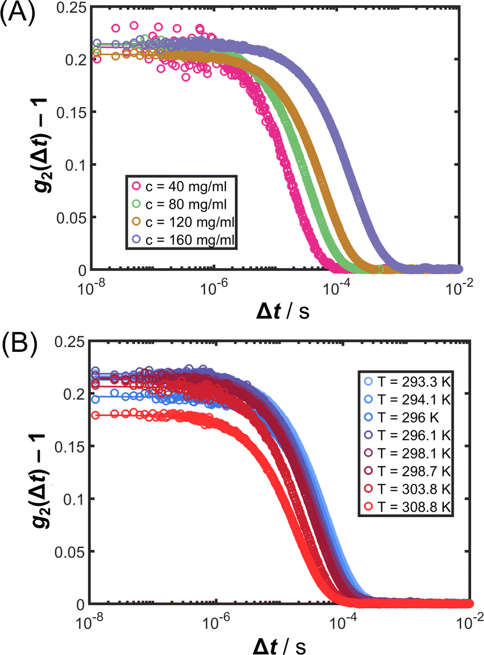 | ||
| Fig. 6 Intensity cross-correlation functions g2(Δt) as a function of the lag time Δt (A) for different protein concentrations (as indicated) at T = 26 °C and (B) for different T (as indicated) at c = 80 mg mL−1: data (symbols) and second-order cumulant fits (lines). | ||
It is important to note that most previous DLS studies on the relaxation rate of concentration fluctuations of proteins close to LLPS72,73,84,85 did not take into account possible effects of multiple scattering; some works86,87 reported non-exponential correlation functions. In the present work, contributions from multiple scattering are suppressed by the 3D cross-correlation set-up and typical single exponential decays of the ISF are observed. In arrested systems, stretched, non-exponential decays are expected,88,89 whereas the (off-)critical slowing down rather results in exponential decays.73,74
Fig. 7(A) shows the T dependence of Γ for different c, as retrieved from fits of eqn (7) and (8) to ISFs. As expected from the inspection of the ISFs in Fig. 6, Γ decreases with increasing c or decreasing T, i.e. the concentration fluctuations exhibit a slowing down upon approaching Ts.
 | ||
| Fig. 7 (A) T dependence of the relaxation rate Γ of lysozyme solutions (0.9 M NaCl, no GuHCl added) with protein concentrations as indicated: experimental data (symbols) and fits to eqn (15) (lines). Inset: Dependence of the correlation length ξc on the correlation length ξ0. Both parameters (symbols) are retrieved from the fits. The line has a slope of 2. (B) Dependence of the relaxation rate Γ on the inverse isothermal compressibility κT, normalized by κ(0)T = 1 (N m−2) (mg mL−1)−1, for various guanidine and protein concentrations indicated as columns and rows in the caption. (C) Dependence of the relaxation rate Γ on the reduced spinodal temperature ε = T/Ts − 1 with the spinodal temperature Ts. Symbols as in (B). The solid line has a slope of 1. | ||
In order to quantitatively understand the observed slowing down, Γ is plotted as a function of κT−1 in Fig. 7(B). A remarkably linear correlation is observed. As in almost all of our experiments, ε is not very small (ε > 0.01) and hence a mean-field picture might be applicable. Then, the relaxation rate Γ and the compressibility κT can be related via:56,90
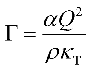 | (14) |
In a more general mode-coupling framework,91–93 the relaxation rate can be described as the sum of a critical and a background contribution in the vicinity of the critical point (or the spinodal). If the correlation length is small compared to Q−1, as for most of our data, the relaxation rate has a simple form:94
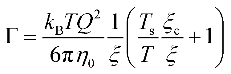 | (15) |
| ξ = ξ0ε−ν | (16) |
3.4 Volume fraction dependence of the relaxation rate of concentration fluctuations: corresponding-states behavior of the collective diffusion coefficient
In order to relate the dynamics to the underlying interactions, it is more convenient to express the relaxation rate of concentration fluctuations in terms of the collective diffusion coefficient Dc. When comparing various solution conditions (additive compositions and temperatures) with each other, it is moreover useful to normalize Dc by the diffusion coefficient of non-interacting single particles, D0. Its value can be obtained from the low c limit of Dc or it can be estimated based on the Stokes–Einstein relation: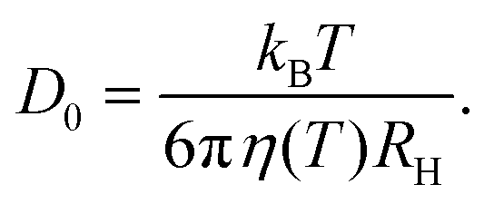 | (17) |
Fig. 8 shows exemplarily data on the ϕ dependence of Dc/D0. As in Fig. 5(A), data for different additive compositions, but the same temperature relative to the critical temperature, T/Tc, are displayed as symbols in the same color. Again, as for κT/κ(id)T, though obtained under different solution conditions, the Dc/D0 data collapse onto a single curve for fixed T/Tc. This indicates a corresponding-states behavior of the collective diffusion coefficient close to Tc. Hence, our data provide further experimental support of the ELCS, also for dynamical properties.
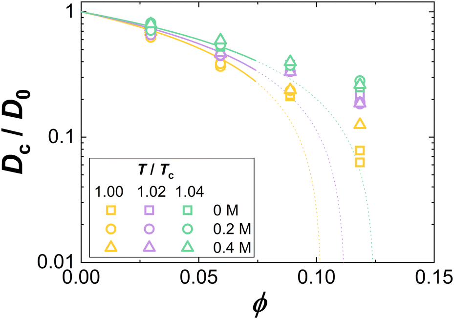 | ||
| Fig. 8 Volume fraction ϕ dependence of the collective diffusion coefficient of concentration fluctuations Dc normalized by the diffusion coefficient at infinite dilution D0. Experimental data for various reduced temperatures T/Tc and guanidine concentrations are marked by symbol color and type, respectively. Lines are computed based on eqn (18) using τ as retrieved from the fits shown in Fig. 5. | ||
As for compressibility data, the simple Baxter model can be applied to analyze the collective diffusion. An approximate equation for Dc(ϕ)/D0, to first order in ϕ,98 is available:
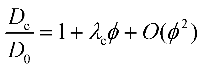 | (18) |
 | (19) |
3.5 Discussion
In this section, the relevance of our findings and their applicability to other solution conditions and other protein systems is commented on with respect to the applicability of the ELCS and the use of coarse-grained colloidal models.The data presented in Fig. 5(A) and 8 indicate that, close to LLPS, the osmotic compressibility and the collective diffusion coefficient is only determined by the volume fraction and the temperature relative to the critical temperature or, equivalently, by the second virial coefficient, as shown in Fig. 5(B). Thus, for our system, the ELCS applies and rationalizes static and dynamical properties of concentrated solutions. It is conceivable that this argument, due to its coarse-grained nature, can be generalized to other globular protein systems. Note that, for the solution conditions investigated here, the repulsive interactions are largely screened and very similar for the various conditions. However, if one considers systems in which repulsion is more important, it is conceivable that this has to be accounted for in an effective particle size.34,39 Nevertheless, the present data as well as previous studies34,47,49,50,82 suggest that the ELCS applies to a broad range of proteins and solution conditions.
The adhesive hard-sphere model proposed by Baxter99 represents one of the simplest systems with short-range attractions. It is therefore astonishing that an approximate theoretical description for this model is suitable to quantitatively describe the complex interactions between protein molecules even in the vicinity of LLPS. While the ELCS suggests that the detailed shape of the interactions does not matter, this does not guarantee that the approximate theoretical description can also be reasonably applied to describe the experimental conditions. It is conjectured that the success of the description might also be related to the globular shape of lysozyme, the moderate concentrations considered as well as the not-to-close proximity to the spinodal. It is conceivable that models accounting for the directionality of the interactions100–102 might be more appropriate to describe the structural and dynamical properties of concentrated solutions of proteins of more complex shape. However, as implied by the ELCS, for the conditions analyzed here, similar results are expected.
4 Conclusion
The extended law of corresponding states suggests that, close to LLPS, thermodynamical properties of protein solutions are not sensitive to the details of the underlying interactions. The present work aims at a comprehensive experimental test of the ELCS. For solution conditions with different protein concentrations, temperatures and additive contents, static and dynamic light scattering experiments were performed. The isothermal osmotic compressibility of the solutions was determined based on the scattered light intensity. From the T dependence of κT, spinodal temperatures Ts were estimated and found to collapse onto a master curve if temperatures are expressed in terms of the second virial coefficient as for the binodals. The intensity cross-correlation function was characterized by a single exponential decay for the conditions studied. The relaxation rate of the concentration fluctuations was found to be correlated with κT. If considered at the same temperature normalized by the critical temperature, values of κT collapse onto a master curve, providing an experimental validation of the ELCS. In addition, a similar collapse is observed for the collective diffusion coefficient. The ϕ dependence of κT and Dc is accurately reproduced by the approximate, analytical expressions for adhesive hard-spheres with interaction parameters that agree with independent data. Our results hence support and broaden the applicability of the ELCS to the static and dynamical properties of protein solutions. They also rationalize and justify the use of coarse-grained colloidal models for protein solutions close to LLPS.Conflicts of interest
There are no conflicts to declare.Acknowledgements
We thank Gerhard Nägele (FZ Jülich, Germany) and Ramón Castañeda-Priego (Leon, Mexico) for stimulating and very helpful discussions. F. P. acknowledges financial support by the German Research Foundation (PL 869/2-1).Notes and references
- J. D. Gunton, A. Shiryayev and D. L. Pagan, Protein condensation. Kinetic pathways to crystallization and disease, Cambridge University Press, 2007 Search PubMed.
- R. Piazza, Curr. Opin. Coll. Interf. Sci., 2004, 8, 515–522 CrossRef CAS.
- P. G. Vekilov, Soft Matter, 2010, 6, 5254–5272 RSC.
- F. Zhang, F. Roosen-Runge, A. Sauter, M. Wolf, R. M. J. Jacobs and F. Schreiber, Pure Appl. Chem., 2014, 86, 191–202 CrossRef CAS.
- J. J. McManus, P. Charbonneau, E. Zaccarelli and N. Asherie, Curr. Opin. Colloid Interface Sci., 2016, 22, 73–79 CrossRef CAS.
- A. Stradner and P. Schurtenberger, Soft Matter, 2020, 16, 307–323 RSC.
- M. Muschol and F. Rosenberger, J. Chem. Phys., 1997, 107, 1953–1962 CrossRef CAS.
- M. L. Broide, T. M. Tominc and M. D. Saxowsky, Phys. Rev. E: Stat. Phys., Plasmas, Fluids, Relat. Interdiscip. Top., 1996, 53, 6325–6335 CrossRef CAS PubMed.
- C. P. Brangwynne, P. Tompa and R. V. Pappu, Nat. Phys., 2015, 11, 899–904 Search PubMed.
- S. Alberti and A. A. Hyman, Nat. Rev. Mol. Cell Biol., 2021, 22, 196–213 CrossRef CAS PubMed.
- A. Pande, J. Pande, N. Asherie, A. Lomakin, O. Ogun, J. King and G. B. Benedek, Proc. Natl. Acad. Sci. U. S. A., 2001, 98, 6116–6120 CrossRef CAS PubMed.
- O. Galkin, K. Chen, R. L. Nagel, R. E. Hirsch and P. G. Vekilov, Proc. Natl. Acad. Sci. U. S. A., 2002, 99, 8479–8483 CrossRef CAS PubMed.
- W. M. Babinchak and W. K. Surewicz, J. Mol. Biol., 2020, 432, 1910–1925 CrossRef CAS PubMed.
- B. A. Salinas, H. A. Sathish, S. M. Bishop, N. Harn, J. F. Carpenter and T. W. Randolph, J. Pharm. Sci., 2010, 99, 82–93 CrossRef CAS PubMed.
- A. S. Raut and D. S. Kalonia, Mol. Pharmaceutics, 2016, 13, 1431–1444 CrossRef CAS PubMed.
- G. A. Vliegenthart and H. N. W. Lekkerkerker, J. Chem. Phys., 2000, 112, 5364–5369 CrossRef CAS.
- O. Galkin and P. G. Vekilov, Proc. Natl. Acad. Sci. U. S. A., 2000, 97, 6277–6281 CrossRef CAS PubMed.
- F. Zhang, F. Roosen-Runge, A. Sauter, R. Roth, M. W. A. Skoda, R. M. J. Jacobs, M. Sztucki and F. Schreiber, Faraday Discuss., 2012, 159, 313–325 RSC.
- F. Zhang, R. Roth, M. Wolf, F. Roosen-Runge, M. W. A. Skoda, R. M. J. Jacobs, M. Stzucki and F. Schreiber, Soft Matter, 2012, 8, 1313–1316 RSC.
- W. C. K. Poon, S. U. Egelhaaf, P. A. Beales, A. Salonen and L. Sawyer, J. Phys.: Condens. Matter, 2000, 12, L569 CrossRef CAS.
- H. Sedgwick, J. E. Cameron, W. C. K. Poon and S. U. Egelhaaf, J. Chem. Phys., 2007, 127, 125102 CrossRef CAS PubMed.
- G. Pellicane, J. Phys. Chem. B, 2012, 116, 2114–2120 CrossRef CAS PubMed.
- C. Gögelein, D. Wagner, F. Cardinaux, G. Nägele and S. U. Egelhaaf, J. Chem. Phys., 2012, 136, 015102 CrossRef PubMed.
- S. Kumar, I. Yadav, D. Ray, S. Abbas, D. Saha, V. K. Aswal and J. Kohlbrecher, Biomacromolecules, 2019, 20, 2123–2134 CrossRef CAS PubMed.
- J. Hansen, R. Uthayakumar, J. S. Pedersen, S. U. Egelhaaf and F. Platten, Phys. Chem. Chem. Phys., 2021, 23, 22384–22394 RSC.
- A. Tardieu, A. Le Verge, M. Malfois, F. Bonneté, S. Finet, M. Riès-Kautt and L. Belloni, J. Cryst. Growth, 1999, 196, 193–203 CrossRef CAS.
- W. Liu, T. Cellmer, D. Keerl, J. M. Prausnitz and H. W. Blanch, Biotechnol. Bioeng., 2005, 90, 482–490 CrossRef CAS PubMed.
- F. Zhang, M. W. A. Skoda, R. M. J. Jacobs, R. A. Martin, C. M. Martin and F. Schreiber, J. Phys. Chem. B, 2007, 111, 251–259 CrossRef CAS PubMed.
- A. J. Chinchalikar, V. K. Aswal, J. Kohlbrecher and A. G. Wagh, Phys. Rev. E: Stat., Nonlinear, Soft Matter Phys., 2013, 87, 062708 CrossRef CAS PubMed.
- M. Wolf, F. Roosen-Runge, F. Zhang, R. Roth, M. W. Skoda, R. M. Jacobs, M. Sztucki and F. Schreiber, J. Mol. Liq., 2014, 200, 20–27 CrossRef CAS.
- M. K. Braun, M. Wolf, O. Matsarskaia, S. Da Vela, F. Roosen-Runge, M. Sztucki, R. Roth, F. Zhang and F. Schreiber, J. Phys. Chem. B, 2017, 121, 1731–1739 CrossRef CAS PubMed.
- S. Kundu, S. Pandit, S. Abbas, V. Aswal and J. Kohlbrecher, Chem. Phys. Lett., 2018, 693, 176–182 CrossRef CAS.
- N. E. Valadez-Pérez, A. L. Benavides, E. Schöll-Paschinger and R. Castañeda-Priego, J. Chem. Phys., 2012, 137, 084905 CrossRef PubMed.
- F. Platten, N. E. Valadez-Pérez, R. Castañeda Priego and S. U. Egelhaaf, J. Chem. Phys., 2015, 142, 174905 CrossRef PubMed.
- D. A. McQuarrie, Statistical mechanics, Harper & Row, New York, 1975 Search PubMed.
- K. S. Pitzer, J. Chem. Phys., 1939, 7, 583–590 CrossRef CAS.
- E. A. Guggenheim, J. Chem. Phys., 1945, 13, 253–261 CrossRef CAS.
- D. R. Schreiber and K. S. Pitzer, Fluid Ph. Equilibria, 1989, 46, 113–130 CrossRef CAS.
- M. G. Noro and D. Frenkel, J. Chem. Phys., 2000, 113, 2941–2944 CrossRef CAS.
- D. Gazzillo and D. Pini, J. Chem. Phys., 2013, 139, 164501 CrossRef PubMed.
- E. Schöll-Paschinger, N. E. Valadez-Perez, A. L. Benavides and R. Castañeda Priego, J. Chem. Phys., 2013, 139, 184902 CrossRef PubMed.
- P. Orea, A. Romero-Martínez, E. Basurto, C. A. Vargas and G. Odriozola, J. Chem. Phys., 2015, 143, 024504 CrossRef CAS PubMed.
- G. Foffi, C. D. Michele, F. Sciortino and P. Tartaglia, Phys. Rev. Lett., 2005, 94, 078301 CrossRef CAS PubMed.
- P. J. Lu, E. Zaccarelli, F. Ciulla, A. B. Schofield, F. Sciortino and D. A. Weitz, Nature, 2008, 453, 499–503 CrossRef CAS PubMed.
- E. Zaccarelli, P. J. Lu, F. Ciulla, D. A. Weitz and F. Sciortino, J. Phys.: Condens. Matter, 2008, 20, 494242 CrossRef.
- N. E. Valadez-Pérez, Y. Liu and R. Castañeda Priego, Phys. Rev. Lett., 2018, 120, 248004 CrossRef PubMed.
- T. Gibaud, F. Cardinaux, J. Bergenholtz, A. Stradner and P. Schurtenberger, Soft Matter, 2011, 7, 857–860 RSC.
- F. Platten, J. Hansen, J. Milius, D. Wagner and S. U. Egelhaaf, J. Phys. Chem. Lett., 2016, 7, 4008–4014 CrossRef CAS PubMed.
- S. Bucciarelli, N. Mahmoudi, L. Casal-Dujat, M. Jehannin, C. Jud and A. Stradner, J. Phys. Chem. Lett., 2016, 7, 1610–1615 CrossRef CAS PubMed.
- J. Hansen, C. Moll, L. López Flores, R. Castañeda Priego, M. Medina-Noyola, S. Egelhaaf and F. Platten, J. Chem. Phys., 2022 DOI:10.1063/5.0128643.
- H. Sedgwick, K. Kroy, A. Salonen, M. B. Robertson, S. U. Egelhaaf and W. C. K. Poon, Eur. Phys. J. E: Soft Matter Biol. Phys., 2005, 16, 77–80 CrossRef CAS PubMed.
- J. Hansen, F. Platten, D. Wagner and S. U. Egelhaaf, Phys. Chem. Chem. Phys., 2016, 18, 10270–10280 RSC.
- C. Tanford and R. Roxby, Biochem., 1972, 11, 2192–2198 CrossRef CAS PubMed.
- F. Platten, J. Hansen, J. Milius, D. Wagner and S. U. Egelhaaf, J. Phys. Chem. B, 2015, 119, 14986–14993 CrossRef CAS PubMed.
- A. Stradner, H. Sedgwick, F. Cardinaux, W. C. K. Poon, S. U. Egelhaaf and P. Schurtenberger, Nature, 2004, 432, 492–495 CrossRef CAS PubMed.
- B. Berne and R. Pecora, Dynamic Light Scattering, Wiley, New York, 1976 Search PubMed.
- L. Hentschel, J. Hansen, S. U. Egelhaaf and F. Platten, Phys. Chem. Chem. Phys., 2021, 23, 2686–2696 RSC.
- C. D. Keefe and S. Mac Innis, J. Mol. Struct., 2005, 737, 207–219 CrossRef CAS.
- J. L. Lundberg, E. J. Mooney and K. R. Gardner, Science, 1964, 145, 1308–1310 CrossRef CAS PubMed.
- T. M. Bender, R. J. Lewis and R. Pecora, Macromol., 1986, 19, 244–245 CrossRef CAS.
- J. Narayanan and X. Liu, Biophys. J., 2003, 84, 523–532 CrossRef CAS PubMed.
- M. Itakura, K. Shimada, S. Matsuyama, T. Saito and S. Kinugasa, J. Appl. Polym. Sci., 2006, 99, 1953–1959 CrossRef CAS.
- J. P. Hansen and I. McDonald, Theory of Simple Liquids, Academic Press, 3rd edn, 2006 Search PubMed.
- C. Urban and P. Schurtenberger, J. Colloid Interface Sci., 1998, 207, 150–158 CrossRef CAS PubMed.
- B. J. Frisken, Appl. Opt., 2001, 40, 4087–4091 CrossRef CAS PubMed.
- K. Schätzel, J. Mod. Optics, 1991, 38, 1849–1865 CrossRef.
- D. E. Koppel, J. Chem. Phys., 1972, 57, 4814–4820 CrossRef CAS.
- A. G. Mailer, P. S. Clegg and P. N. Pusey, J. Phys.: Condens. Matter., 2015, 27, 145102 CrossRef PubMed.
- M. C. Jenkins and S. U. Egelhaaf, Adv. Coll. Interf. Sci., 2008, 136, 65 CrossRef CAS PubMed.
- J. A. Thomson, P. Schurtenberger, G. M. Thurston and G. B. Benedek, Proc. Natl. Acad. Sci. U. S. A., 1987, 84, 7079–7083 CrossRef CAS PubMed.
- D. N. Petsev, X. Wu, O. Galkin and P. G. Vekilov, J. Phys. Chem. B, 2003, 107, 3921–3926 CrossRef CAS.
- M. Manno, C. Xiao, D. Bulone, V. Martorana and P. L. San Biagio, Phys. Rev. E: Stat., Nonlinear, Soft Matter Phys., 2003, 68, 011904 CrossRef PubMed.
- M. Manno, D. Bulone, V. Martorana and P. L. S. Biagio, J. Phys.: Condens. Matter, 2004, 16, S5023–S5033 CrossRef CAS.
- S. Bucciarelli, L. Casal-Dujat, C. De Michele, F. Sciortino, J. Dhont, J. Bergenholtz, B. Farago, P. Schurtenberger and A. Stradner, J. Phys. Chem. Lett., 2015, 6, 4470–4474 CrossRef CAS PubMed.
- R. Piazza, V. Peyre and V. Degiorgio, Phys. Rev. E: Stat. Phys., Plasmas, Fluids, Relat. Interdiscip. Top., 1998, 58, R2733–R2736 CrossRef CAS.
- B. Barboy, J. Chem. Phys., 1974, 61, 3194–3196 CrossRef CAS.
- C. Regnaut and J. C. Ravey, J. Chem. Phys., 1989, 91, 1211–1221 CrossRef CAS.
- S. V. G. Menon, C. Manohar and K. S. Rao, J. Chem. Phys., 1991, 95, 9186–9190 CrossRef CAS.
- S. V. G. Menon, V. K. Kelkar and C. Manohar, Phys. Rev. A, 1991, 43, 1130–1133 CrossRef CAS PubMed.
- S.-H. Chen and P. Tartaglia, Scattering Methods in Complex Fluids, Cambridge University Press, 2015 Search PubMed.
- A. Santos, A Concise Course on the Theory of Classical Liquids, Springer, Cham, 2016 Search PubMed.
- J. Hansen, J. N. Pedersen, J. S. Pedersen, S. U. Egelhaaf and F. Platten, J. Chem. Phys., 2022, 156, 244903 CrossRef CAS PubMed.
- H. E. Stanley, Introduction to Phase Transitions and Critical Phenomena, Clarendon Press, 1971 Search PubMed.
- T. Tanaka, C. Ishimoto and L. T. Chylack, Science, 1977, 197, 1010–1012 CrossRef CAS PubMed.
- C. Ishimoto and T. Tanaka, Phys. Rev. Lett., 1977, 39, 474–477 CrossRef CAS.
- B. M. Fine, J. Pande, A. Lomakin, O. O. Ogun and G. B. Benedek, Phys. Rev. Lett., 1995, 74, 198–201 CrossRef CAS PubMed.
- B. M. Fine, A. Lomakin, O. O. Ogun and G. B. Benedek, J. Chem. Phys., 1996, 104, 326–335 CrossRef CAS.
- R. Bandyopadhyay, D. Liang, J. L. Harden and R. L. Leheny, Solid State Commun., 2006, 139, 589–598 CrossRef CAS.
- A. Madsen, R. L. Leheny, H. Guo and M. S. O. Czakkel, New J. Phys., 2010, 12, 055001 CrossRef.
- H. L. Swinney and D. L. Henry, Phys. Rev. A, 1973, 8, 2586–2617 CrossRef CAS.
- K. Kawasaki, Ann. Phys., 1970, 61, 1–56 CAS.
- D. W. Oxtoby and W. M. Gelbart, J. Chem. Phys., 1974, 61, 2957–2963 CrossRef CAS.
- H. C. Burstyn and J. V. Sengers, Phys. Rev. A, 1982, 25, 448–465 CrossRef CAS.
- C. M. Sorensen, J. Phys. Chem., 1988, 92, 2367–2370 CrossRef CAS.
- J. Kestin, H. E. Khalifa and R. J. Correia, J. Phys. Chem. Ref. Data, 1981, 10, 71–88 CrossRef CAS.
- K. Kawahara and C. Tanford, J. Biol. Chem., 1966, 241, 3228–3232 CrossRef CAS PubMed.
- M. Muschol and F. Rosenberger, J. Chem. Phys., 1995, 103, 10424–10432 CrossRef CAS.
- B. Cichocki and B. U. Felderhof, J. Chem. Phys., 1990, 93, 4427–4432 CrossRef CAS.
- R. J. Baxter, J. Chem. Phys., 1968, 49, 2770–2774 CrossRef CAS.
- C. Gögelein, G. Nägele, R. Tuinier, T. Gibaud, A. Stradner and P. Schurtenberger, J. Chem. Phys., 2008, 129, 085102 CrossRef PubMed.
- F. Roosen-Runge, F. Zhang, F. Schreiber and R. Roth, Sci. Rep., 2014, 4, 7016 CrossRef CAS PubMed.
- N. Skar-Gislinge, M. Ronti, T. Garting, C. Rischel, P. Schurtenberger, E. Zaccarelli and A. Stradner, Mol. Pharmaceutics, 2019, 16, 2394–2404 CrossRef CAS PubMed.
| This journal is © the Owner Societies 2023 |