Avoiding some common mistakes in straight line regression. Part 1

Abstract

Analytical scientists generate and use bivariate experimental data mostly in two distinct application areas. In a quantitative calibration experiment standard materials are used to establish a calibration line that can be applied to estimate the concentrations of test samples. A second source of bivariate data is in the comparison of two analytical methods, often for validation purposes: results from the two methods as applied to the same set of test materials are plotted against each other in the hope of obtaining an excellent straight line fit to demonstrate agreement between them. There are several ways of deriving a straight line from bivariate data: the best will depend on which of these applications is involved and on the methods used in assembling the data. In practice a straight line may not be an adequate model for the data, but even if it is, regression methods are often misused and misinterpreted.

---

Regression basics

The simplest and most commonly used model for summarising bivariate data as a straight line (y = a + bx) is the regression method known as Ordinary Least Squares (OLS). It provides estimates a and b of the supposed true values of the intercept α and the slope β of the line. (Note that these estimates are not independent of each other – see AMC Technical Brief No. 87.)¹ In calibration, the analyst utilises a set of materials of known composition which provide the x values – the predictor or independent variable. Such calibrators should obviously be chosen to cover the expected range of the analyte concentrations and with even spacing between them: commonly up to 6–10 calibrators are used. (The calibrators should be truly independent of each other, so making them up by serial dilutions, for example, is inappropriate.) Each calibrator provides an analytical result y, the response or dependent variable; these experimental y-values are subject to measurement errors. The OLS slope and intercept estimates are calculated by minimising the sum of the squared residuals, i.e., the differences between the experimental y-values and the y-values on the fitted line at the corresponding x-values (hence the term “least squares” often applied to this method). Residuals, readily obtained from computer programs or spreadsheets, have important diagnostic value (see below). The calculated line (Fig. 1) can be used to estimate the concentrations of test materials, provided they are effectively matrix-matched and studied under the same conditions as the standards. (The data used in Fig. 1–3 are from set 8 in the AMC Datasets resource on the Royal Society of Chemistry’s platform).²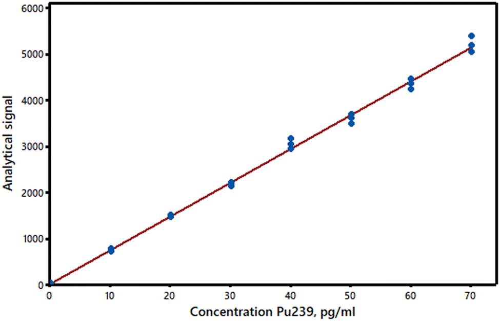

Fig. 1 A typical straight line calibration experiment with replicate values for each calibrator.

The

OLS line calculated using these principles is called the line of regression of y on x as we assume that the x-values are known exactly. It also assumes that there is an underlying straight line relationship between the predictors and responses, and that the (unknown) variance in each (y) response is normally distributed, and the same at every value of the predictor (x), (i.e., it is not a function of concentration). The latter situation is called homoscedasticity.

Most of the misuse of regression arises from departures in the dataset from one or more of these assumptions. In other subject areas the line of regression of y on x is normally used to predict y-values from known x-values. (For example, a graph showing the relationship between the heights [y] of some children of known ages [x] would be used to indicate whether another child of known age x was above or below the expected height y.) Analytical scientists do the opposite (so-called inverse regression, predicting x-values from y-values), and this has consequences when we calculate the uncertainty of a concentration estimated from a calibration line (see AMC Technical Brief No. 22).³ We notice also that OLS is not really a sound approach to handling method comparison data, since both x- and y-values are subject to measurement variation in such cases (see AMC Technical Brief No. 10).⁴

Departures from assumptions and their consequences

(1) The true relationship between response and concentration deviates from a straight line. If the true relationship between the analyte concentrations and the response values is really a curve there will be a lack of fit between the data and the OLS straight line. (In some analytical methods the true relationship is in principle curved, but at low concentrations the curvature is so small that a straight line plot is an excellent approximation.) Curvature can sometimes be detected, or at least suspected, by visual inspection of a calibration plot, but any method for detecting a significant lack of fit may have a low power for calibration sets of a typical size. In particular, the use of the Pearson correlation coefficient, r, or the related R² statistic is not recommended as they may show values closely approaching unity even with plots that are clearly curved (see AMC Technical Brief No. 3).⁵ We can, however, make use of the y-residuals, which can be plotted against the predictor variable (Fig. 2). The residuals should have randomly distributed positive and negative signs if a straight line is suitable for calibration purposes. Moreover, if the above assumptions are valid and a straight line plot is appropriate the residuals should be normally distributed about zero. (Apart from rounding errors, the residuals will always sum to zero.) If replicate measurements of the response variable are made for each predictor value (this is an invaluable but far from common practice in validation) then analysis of variance (ANOVA) can be applied to compare the pure error due to experimental variation with the variation due to lack of fit. Lastly, it may be worthwhile to see if a markedly better fit is obtained by fitting a second-order polynomial to the data, in which case the adjusted R² statistic R′² will be higher for the polynomial than for the straight line model. Details of these methods are given in standard texts. Importantly, in calibration experiments a lack of fit at very low concentrations can cause serious relative errors and misleading estimates of detection limits. A lack of fit can also be caused by factors other than curvature, e.g., the use of unmatched matrix reference materials to set up the predictor values.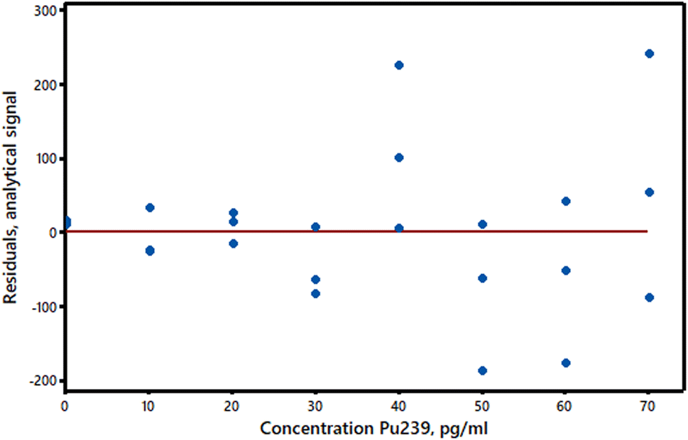

Fig. 2 Residuals plot for the calibration data in Fig. 1.

(2) The variance of the y-values is not the same at all x-values. This common situation is called heteroscedasticity and is easily detected if the y-residuals are plotted against the response variable values. Most frequently, the y-value variance increases with analyte concentration (Fig. 2 suggests that this may be the case in our example). If the variance at each y-value can be estimated (even roughly) from replicate measurements, or if the extent of the heteroscedasticity is known from previous similar experiments, then weighted regression calculations can be used (see AMC Technical Brief No. 27).⁶ These calculations are rather more complex than OLS ones, but are readily accessible in software packages and Excel® add-ins. While heteroscedasticity may not be very important in short range calibration experiments, it can have the effect of substantially increasing the standard error of the intercept of the calibration graph, with corresponding effects on the estimated detection limit. A second approach to heteroscedasticity is available if the standard deviations of the y-values are more or less proportional to the values themselves. A log transformation will then harmonise the variances so that conventional OLS methods can be applied (Fig. 3).

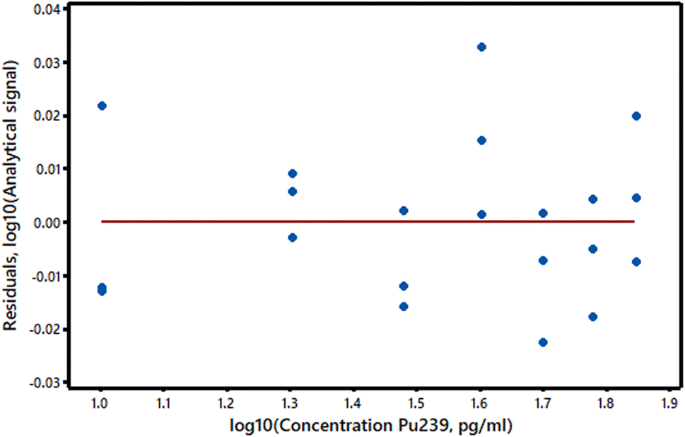Fig. 3 Logarithmic transformation of the residuals and concentrations of the data in Fig. 1.

Other hazards

In addition to the problems of non-linearity and heteroscedasticity there are several other aspects of regression methods that can lead to mistakes in data interpretation. (One obvious mistake would be to plot the x- and y-values the wrong way round!) Moreover, as we have seen, the OLS approach is often unsuitable for method comparison studies, so alternative methods are highly desirable in such cases. These issues will be discussed further in a subsequent Technical Brief.

This Technical Brief was prepared by Professors M. Thompson (Birkbeck University of London) and J. N. Miller (Loughborough University) on behalf of the Statistics Expert Working Group of the Analytical Methods Committee and approved by the AMC on 6th October 2023.

References

1. Analytical Methods Committee, The correlation between regression coefficients: combined significance testing for calibration and quantitation of bias, AMC Technical Brief No. 87, Anal. Methods, 2019, 11, 1845,  10.1039/c9ay90041a.
2. Analytical Methods Committee, AMC Datasets a resource for analytical scientists, AMC Technical Brief No. 72, Anal. Methods, 2016, 8, 1741,  10.1039/c6ay90016j , https://www.rsc.org/membership-and-community/connect-with-others/join-scientific-networks/subject-communities/analytical-science-community/amc/datasets/.
3. Analytical Methods Committee, Uncertainties in concentrations estimated from calibration experiments, AMC Technical Brief No. 22, March 2006, https://www.rsc.org/membership-and-community/connect-with-others/join-scientific-networks/subject-communities/analytical-science-community/amc/technical-briefs/.
4. Analytical Methods Committee, Fitting a linear functional relationship to data with error on both variables, AMC Technical Brief No. 10, March 2002, https://www.rsc.org/membership-and-community/connect-with-others/join-scientific-networks/subject-communities/analytical-science-community/amc/technical-briefs/.
5. Analytical Methods Committee, Is my calibration linear?, AMC Technical Brief No. 3, December 2005, https://www.rsc.org/membership-and-community/connect-with-others/join-scientific-networks/subject-communities/analytical-science-community/amc/technical-briefs/.
6. Analytical Methods Committee, Why are we weighting? AMC Technical Brief No. 27, June 2007, https://www.rsc.org/membership-and-community/connect-with-others/join-scientific-networks/subject-communities/analytical-science-community/amc/technical-briefs/.

---