
 Open Access Article
 This Open Access Article is licensed under a
 Creative Commons Attribution 3.0 Unported Licence
Removing non-resonant background from broadband CARS using a physics-informed neural network†
Ryan
Muddiman
 a,
Kevin
O' Dwyer
a,
Charles. H.
Camp
Jr
b and
Bryan
Hennelly
*ac
a,
Kevin
O' Dwyer
a,
Charles. H.
Camp
Jr
b and
Bryan
Hennelly
*ac
aDepartment of Electronic Engineering, Maynooth University, Co. Kildare, Ireland
bBiosystems and Biomaterials Division, National Institute of Standards and Technology, Gaithersburg, MD, USA
cDepartment of Computer Science, Maynooth University, Co. Kildare, Ireland
First published on 31st July 2023
Abstract
Broadband coherent anti-Stokes Raman scattering (BCARS) is capable of producing high-quality Raman spectra spanning broad bandwidths, 400–4000 cm−1, with millisecond acquisition times. Raw BCARS spectra, however, are a coherent combination of vibrationally resonant (Raman) and non-resonant (electronic) components that may challenge or degrade chemical analyses. Recently, we demonstrated a deep convolutional autoencoder network, trained on pairs of simulated BCARS-Raman datasets, which could retrieve the Raman signal with high quality under ideal conditions. In this work, we present a new computational system that incorporates experimental measurements of the laser system spectral and temporal properties, combined with simulated susceptibilities. Thus, the neural network learns the mapping between the susceptibility and the measured response for a specific BCARS system. The network is tested on simulated and measured experimental results taken with our BCARS system.
1. Introduction
Coherent anti-Stokes Raman scattering (CARS) is an established technique which can probe vibrational states in material providing contrast for sample identification, cell diagnostics and imaging. This technique relies on the coherent excitation and scattering of light using a single vibrational resonance. Broadband CARS (BCARS) is an evolution of the CARS technique, which allows the whole vibrational spectrum of a sample to be probed with a single acquisition.1 This typically utilizes a broadband laser pulse for coherent excitation of a wide frequency region and a narrowband probe pulse that scatters off this excitation. This configuration has enabled the demonstration of high-speed Raman hyperspectral imaging of biological tissues with 3 ms acquisition time per pixel.2The BCARS signal is generated through the interference of two optical pulses and the third-order electric susceptibility of the sample χ(3). The intensity is proportional to the squared susceptibility, therefore the detected signal is quadratic in the sample concentration. The susceptibility contains a contribution from vibrational resonances within the molecule as well as a non-resonant component known as the non-resonant background (NRB). The sample electron response to the incident fields is responsible for the NRB and is generated via four-wave mixing. The coherent interference of the NRB and the vibrationally resonant response gives rise to asymmetric lineshapes in the BCARS signal intensity and as such obscures the relative species concentration. This property of BCARS measurements is a well-known drawback for which multiple experimental and mathematical-based methods have been produced for its treatment. Experimental methods involve for example controlling the excitation and detection polarization angle3 (P-CARS), frequency-modulation CARS (FM-CARS)4 and time-resolved CARS (T-CARS).5 These methods although useful, add to the complexity of the measurement and in some instances suppress the resonant contribution during the process.
Another approach for recovering the resonant susceptibility is to use BCARS intensity data and mathematical relationships between the phase and intensity of the BCARS signal. One such method involves the fact that the susceptibility obeys causality and therefore the Kramers–Kronig relations of a BCARS measurement can be used to provide the phase of χ(3) as demonstrated by Liu et al.6 In practice, this method requires pre-processing of the spectra, either using the singular value decomposition as a denoising and spectral encoding step as shown by Masia et al.7 or a baseline correction of the retrieved phase due to errors from the finite frequency range of actual measurements and the use of a surrogate NRB.8 Another approach is the maximum entropy method (MEM) which computes χ(3) through maximisation of the entropy of an autocorrelation function, whose parameters are consistent with the measured data.9 This method requires prior information of at least two locations in the spectrum that the phase is known, in order for proper retrieval, as well as a measurement of the NRB. Since baseline correction is a supervised technique and prior information is required for the MEM, both of these methods must also be supervised for Raman signal extraction. Thus, the current mathematical approaches are unsuitable for bulk phase retrieval of unknown BCARS spectra.
Another emerging technique for NRB removal is to use a deep learning network to recover the Raman spectrum directly from BCARS measurements. This has been demonstrated first by Valensise et al. using purely synthetic BCARS data which was used to train a convolutional neural network (CNN).10 Long-short term memory (LSTM) networks were also applied to this problem, with the performance of the network tested on real spectra.11 Saghi et al.12 then demonstrated improved retrieval using semi-synthetic training data and fine-tuning an already trained network. A comparison with the performance of the MEM approach was also shown. The semi-synthetic data were generated using actual recordings of Raman spectra, with an NRB generated mathematically using sigmoid functions.
In our previous paper,13 we trained a CNN called VECTOR on paired CARS intensity data and its respective Raman intensity. The CARS spectra were simulated assuming a spectrally flat excitation. The stimulation profile from the laser sources has a profound effect on the CARS spectra generated, and this impacted negatively on the networks ability to remove the NRB from real BCARS measurements. In this paper, we introduce VECTOR2, whereby the training set is produced using a synthetically generated susceptibility; however, we also take into account the effect of laser pulse characteristics on the spectral shape. Two processing steps are applied to the synthetic susceptibility in accordance with the physical model. Firstly the laser stimulation profile, which can be measured experimentally, is used to modulate the susceptibility, and secondly the probe laser spectrum is convolved with the result. Thus, we more accurately mimic the effect of a given system in simulating a spectrum.
2. BCARS
2.1 Theory
The CARS process occurs due to nonlinear four-wave mixing of light in matter. In CARS, a pulse pair called the pump and Stokes at frequencies ωP, ωS generates a vibrational coherence within a molecule at frequency Ω = ωP − ωS and a probe pulse at frequency ωpr scatters from this coherence producing radiation at the frequency ωpr + Ω. The process is parametric and therefore no energy transfer between photons or the molecule occurs. When the Stokes pulse has a broadband spectrum, the produced radiation is that of a broadband CARS spectrum. In bulk matter, the phases of the input and output light must match for the nonlinear interaction to appreciably build. Phase-matching is most commonly achieved using tight-focusing of the input beams with a relatively high numerical aperture objective. The large range of exit angles thus generates a wide range of wave-vector directions that satisfy phase-matching of the interaction.In CARS, the third-order nonlinear susceptibility χ(3) is probed. This susceptibility is defined as the sum of a resonant part that is complex and a purely real non-resonant part
 | (1) |
In BCARS, it is the squared magnitude of the susceptibility modulated by the laser profile that is detected, as given by eqn (2)
| ICARS ∝ |[χ(3)(ES × EP)] * Epr|2 | (2) |
2.2 Experimental system
Our BCARS system consists of a FemtoFiber PRO master-oscillator power amplifier (MOPA) mode-locked laser system at 1550 nm that is frequency doubled using periodically-poled lithium niobate (PPLN) to generate a narrowband probe pulse. The master laser operates at a repetition rate of 40 MHz. The amplified seed is coupled into a highly nonlinear fiber (HNF) which causes spectral broadening due to Kerr effects, generating the Stokes pulse. The Stokes spans approximately 900–1400 nm. We use an external prism pair pulse compressor utilizing two SF10 prisms for compensating for group velocity dispersion. The microscope contains a motorized XYZ stage (applied scientific instrumentation) which is controlled by MicroManager through a MATLAB interface. The beams are overlapped using a dichroic and coupled in to the microscope with a high-NA objective (UPlanSApo 60×/1.20, Olympus) and the transmitted light is collected using a second objective (UMPlanFl 20×/0.46, Olympus). The excitation light is filtered using a high-pass filter (FESH 0750, Thorlabs). The filtered anti-Stokes light is then coupled into a spectrograph (Shamrock 500i-A, Andor Technology Ltd.) and recorded using a Peltier cooled CCD operating at −80 °C (Newton 920, Andor Technology Ltd.). The system incorporates a 300 L mm−1 grating and full vertical binning (FVB) with a recording range from 443 to 4489 cm−1. A diagram of our system is shown in Fig. 1. | ||
| Fig. 1 BCARS microscope setup (D: diode, SAM: saturable absorber mirror, EDFA: erbium-doped fiber amplifier, HNF: highly nonlinear fiber, PC: pulse compressor, DM: dichroic mirror, BPF: 766 bandpass filter, HPF: 750 nm highpass filter, CCD: charge-coupled device). | ||
2.3 Conventional phase retrieval
In conventional BCARS measurements, χ(3) or its imaginary part is sought, when ICARS is known. However, since the unknown NRB interferes with the resonant susceptibility during scattering, there is no simple relation between the BCARS intensity and Im(χ(3)). Since the laser profile can be measured, |χ(3)|2 can be approximately determined from ICARS, since| ICARS ∝ |Sχ(3)|2 ≈ |S|2|χ(3)|2 | (3) |
 | (4) |
It has been shown that the Kramers–Kronig (KK) method allows quantitative and reliable extraction of the Raman spectrum of neat chemicals and tissues.8 The KK relation is built on the relation that the real and imaginary parts of an analytic function are related. In common usage, the Bode gain-phase relation is employed14
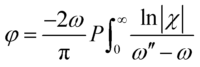 | (5) |
The main problem of the current technique is the requirement of a surrogate NRB reference spectrum. If the NRB is not purely real, then any absorbance or scattering will affect the NRB spectrum. The implementation of a windowed Hilbert transform for performing the KK relation also results in an approximately additive error term in the retrieved spectral phase of the susceptibility. The removal of this baseline through detrending is a method requiring supervision, since the error term depends on the window size. Classical methods are also susceptible to noise, since any detrending method will be affected by noise present in the phase, and thus often statistical denoising is employed using many BCARS spectra in order to prepare the spectra for phase retrieval. The retrieval of the susceptibility through KK also assumes that the probe spectrum is significantly narrower than the resonant linewidths.
Using deep learning for phase retrieval has multiple benefits; firstly, deep neural networks are very accurate function approximators. Secondly, they have the capability to perform efficient dimensionality reduction. It has been shown that a single hidden layer autoencoder network solves the same problem as singular value decomposition (SVD).15 This is due to the fact that the loss function is equal to the SVD objective function. Deep learning approaches also make no assumption of the phase of S, and the full electric field can be included to reproduce complex laser phase conditions. This is discussed in more detail in the ESI.† This approach also makes no assumption on the probe shape, as this is included in the simulation. This could possibly be beneficial in terms of the deconvolution process inherent to VECTOR2.
3. VECTOR2 deep learning network architecture
Here, we provide a brief description of our architecture; a more complete description is provided in our original paper.13 Our deep-learning network is of the class known as deep autoencoders. An autoencoder (AE) is a network that learns how to efficiently encode its input to a hidden (often lower dimensional) representation in latent space and then reconstruct, or decode, the input again from this representation. The autoencoder output dimension is equal to its input and so it is ideal for low-dimensional approximation of signals. Including a low dimensional hidden layer prevents the network from learning the identity function, since their goal is to determine a mapping from the input to the output. When used for dimensionality reduction, the training loss might simply be given as a sparsity metric such as![[small script l]](https://www.rsc.org/images/entities/i_char_e146.gif) 0 or 1 loss of the output and input. When the loss is applied to the output and some other function (for example a noise free version of the input), then the network will be trained to find the mapping between the input and the transformed output given. A 6-layer autoencoder network is illustrated in Fig. 2, although practically we employ 18 layers. The layer properties are shown in Table 1. Autoencoders are commonly symmetric, meaning a network with n total layers will have its kth and (n − k + 1) layer equal in size. Dimensionality reduction is achieved through forcing the input through the constricted layer by reducing its size iteratively. Typical AEs incorporate only fully-connected layers for both the encoder and decoder.16
0 or 1 loss of the output and input. When the loss is applied to the output and some other function (for example a noise free version of the input), then the network will be trained to find the mapping between the input and the transformed output given. A 6-layer autoencoder network is illustrated in Fig. 2, although practically we employ 18 layers. The layer properties are shown in Table 1. Autoencoders are commonly symmetric, meaning a network with n total layers will have its kth and (n − k + 1) layer equal in size. Dimensionality reduction is achieved through forcing the input through the constricted layer by reducing its size iteratively. Typical AEs incorporate only fully-connected layers for both the encoder and decoder.16
 | ||
| Fig. 2 Diagram of the autoencoder network and BCARS generation procedure. | ||
| Stage | O (K, Cin, Cout, S) | n(T × C) | |
|---|---|---|---|
| Input | — | 1000 × 1 | |
| Encoder | Layer 1 | 8, 1, 64, 1 | 993 × 64 |
| Layer 2 | 8, 64, 128, 2 | 493 × 128 | |
| Layer 3 | 8, 128, 256, 2 | 243 × 256 | |
| Layer 4 | 8, 256, 512, 2 | 118 × 512 | |
| Layer 5 | 8, 512, 1024, 2 | 56 × 1024 | |
| Layer 6 | 8, 1024, 2048, 2 | 25 × 2048 | |
| Layer 7 | 8, 2048, 2048, 2 | 18 × 2048 | |
| Layer 8 | 8, 2048, 2048, 2 | 11 × 2048 | |
| Layer 9 | 8, 2048, 2048, 2 | 4 × 2048 | |
| Latent space | — | 4 × 2048 | |
| Decoder | Layer 1 | 8, 2048, 2048, 2 | 11 × 2048 |
| Layer 2 | 8, 2048, 2048, 2 | 18 × 2048 | |
| Layer 3 | 8, 2048, 2048, 2 | 25 × 2048 | |
| Layer 4 | 8, 2048, 1024, 2 | 56 × 1024 | |
| Layer 5 | 8, 1024, 512, 2 | 118 × 512 | |
| Layer 6 | 8, 512, 256, 2 | 243 × 256 | |
| Layer 7 | 8, 256, 128, 2 | 493 × 128 | |
| Layer 8 | 8, 128, 64, 2 | 993 × 64 | |
| Layer 9 | 8, 64, 1 | 1000 × 1 | |
| Output layer | Sigmoid | 1000 × 1 | |
Here, we use our previously designed architecture, VECTOR,13 which incorporates convolutional layers instead of fully-connected layers as well as symmetric skip connections17–19 between each paired convolutional layer and transposed convolutional layer in the encoder and the decoder respectively. We previously demonstrated that skip connections significantly boosted performance for deeper networks such as the one used in this paper. Skip connections allow some features in the input or in shallow layers to propagate through the network and bypass the low-dimensional latent space. This property allows high-level features to be preserved that might otherwise fail to be preserved by the latent space.
This previous network performed Raman extraction on fully synthetic BCARS spectra that had a spectrally flat excitation; the input was the ideal BCARS spectrum and the 1 loss function was applied to the output and the true Raman spectrum. The performance of this previous network was poor when applied to real BCARS spectra because non-material dependent artefacts, such as the stimulation spectrum or probe shape were not present in the training data. Therefore, the network had no information about the optical system generating the spectra. Our solution to this is to generate BCARS training spectra using the actual laser stimulation profile of our BCARS microscope as illustrated in Fig. 2, which is the core subject of this manuscript. The details of which are given in Section 4. Implementing the system parameters in the training samples provided much more realistic BCARS training data from which the network can learn. Although we have previously demonstrated the VECTOR architecture for BCARS NRB removal in ref. 13, there are several points regarding the novelty in its usage in this paper. The primary novelty is the use of training sets of simulated BCARS spectra that include the specific stimulation profile of the BCARS system. The resultant network performs optimally for a specific system. Another point of novelty is that the convolution of the probe is also included in the simulated training sets. The result is that the network will perform deconvolution and the resolution of the retrieved spectra will be enhanced. A custom loss function has also been designed for these new training sets to better accommodate the significant disparity that can exist for resonance amplitudes in the fingerprint and CH-stretching regions of the Raman spectrum.
4. Simulating BCARS training data using measured system response
4.1 Simulating the susceptibility
Realistic Raman spectra were produced by generating sub-spectra in three different frequency regions: the fingerprint, the CH-stretch, and the OH-stretch regions. The fingerprint region was characterised by many narrow peaks that spanned 600–1800 cm−1. The CH-stretch region, spanning 2900–3500 cm−1, had fewer peaks but each with significantly higher amplitudes. Finally, we also simulated the OH-stretch region as a single broad peak from approximately 3200–3400 cm−1.The resonant susceptibility for each region was generated as a sum of individual complex Lorentzians as follows:
 | (6) |
| Dataset | |||||
|---|---|---|---|---|---|
| Component | Symbol | Name | Unit | VECTOR-MU-sparse | VECTOR-MU-dense |
| NRB | ω NRB | NRB centre frequency | THz | U(600, 800) | |
| σ NRB | NRB width | THz | U(400, 500) | ||
| β | NRB amplitude | — | U(0.3, 0.5) | ||
| Noise | SNR | SNR (relating to shot noise) | — | U(200, 1000) | |
| σ read | Gaussian additive noise (std) | — | U(0.00001, 0.0001) | ||
| Distortion | A | Ripple amplitude | — | U(0, 0.02) | |
| T | Ripple frequency | Pixels | U(50, 1000) | ||
| Φ | Ripple phase | — | U(0, π) | ||
| Fingerprint | a | Amplitude | — | U(0, 0.1) | |
| N | Number of peaks | — | U(1, 15)∈![[Doublestruck Z]](https://www.rsc.org/images/entities/char_e17d.gif) |
U(1, 50)∈ |
|
| Γ | Half-width | cm−1 | U(2, 10) | U(2, 75) | |
| Ω | Resonant frequency | cm−1 | U(600, 1800) | ||
| CH-region | a | Amplitude | — | U(0, 1) | |
| N | Number of peaks | — | U(0, 3)∈ |
||
| Γ | Half-width | cm−1 | U(2, 30) | ||
| Ω | Resonant frequency | cm−1 | U(2900, 3500) | ||
The non-resonant susceptibility was generated using a wide Gaussian for the shape:
 | (7) |
 and
and  were normalized over the band corresponding to the CCD using the maximum of their absolute values. After normalization, we scaled the resonant susceptibility by a scaling factor β and the non-resonant susceptibility by 1 − β. The β parameter is designed to control the relative amplitude of the two components of the susceptibility, and is randomly selected from a uniform distribution in the range of 0.3 to 0.5. The total susceptibility was then generated according to eqn (1). Note that the true Raman spectrum, IRaman used in the loss function is defined as the imaginary part of
  :
: | (8) |
4.2 Including the system-specific stimulation profile
After generating the susceptibility, this is multiplied by the laser stimulation profile, S, and the result is convolved with the probe pulse Epr as described in eqn (2). We propose two methods to obtain S and Epr with relative advantages/disadvantages. The first method involves cross-correlation frequency resolved optical gating (XFROG), as described by Selm20 which returns the electric fields ES and Epr from which S can be calculated exactly.In Fig. 3(a), the XFROG spectrogram is shown for our system, including the temporal profile at 578.2 nm, corresponding to the envelope of Epr. This function can be used to obtain Epr which is shown in Fig. 3(b). The estimate of ES (amplitude and phase) is shown in Fig. 3(c), from which it can be seen that the phase is flattened over the width of the pulse. In Fig. 3(d) shows the resulting amplitude and phase of the stimulation profile S = ES × EP, which are calculated using ES and Epr as described in the figure caption. It is notable that the amplitude in the 2-colour region of the stimulation profile is relatively weak compared to the 3-colour region. Similar systems have been reported to produce a much stronger amplitude in this region21 and it is likely the amplitude of our system could be increased by optimising the laser spectrum. Nevertheless, the amplitude is sufficient to capture resonance effects in the 2-colour region as demonstrated in Section 4.
 | ||
| Fig. 3 (a) XFROG spectrogram of two-colour region with marginal plot at the reference wavelength of 578.2 nm (smoothed using a Savitzky–Golay filter of window size 9 and order 3); (b) probe pulse amplitude obtained from the discrete Fourier transform of the marginal plot in (a). Also shown in this figure is the result of modelling the amplitude as a Gaussian function based on the laser specification – centre at 770 nm and FWHM 0.58 nm; (c) Stokes pulse intensity and phase obtained from the retrieval method; (d) amplitude of stimulation profile obtained using two methods: firstly the ES and Epr obtained from XFROG are used to generate S = ES × EP where EP is given by ES and Epr for the 3- and 2-colour regions, respectively. This method also enables the phase of S to be obtained; secondly, the amplitude of S is estimated using the square root of a glass spectrum. This method does not permit measurement of the phase. | ||
A simpler method also exists to estimate S and Epr. The latter can simply be modelled using a Gaussian function with a standard deviation related to the full width half maximum of the spectrum, often provided by the laser manufacturer. The result of this approach is also shown in Fig. 3(b) and is found to be in good agreement with the XFROG method. Estimating S involves recording a BCARS spectrum from a non-resonant material such as glass, and taking the square root. Any measurement of the four-wave mixing response in a medium with no electronic or Raman resonances results in  and is real valued. It follows that
  . If the amplitude of the NRB is assumed to be approximately flat, ES is assumed to have an approximately flat phase, and Epr is assumed to be sufficiently narrow, then it follows that
  The result of this approach is shown in Fig. 3(d) in which it can be seen there is good agreement with the XFROG method.
Both of the methods described above provide values for S and Epr. The XFROG method has the advantage of providing the phase of S; however, if this phase is flat (which is true for the three and two-colour regions in Fig. 3) then this advantage may be overlooked. The second method has the advantage of being simpler, requiring only a single non-resonant spectrum. The second method also has the very significant advantage of including the same sensitivity response of the spectrometer with respect to the BCARS spectra. This cannot be said for the XFROG method, which involves recording spectra in a different band of wavelengths. We believe that the slight difference in the estimates for S that can be observed in Fig. 3(d) can be attributed to this difference. Therefore, the use of S obtained directly from glass is preferable as this will provide self-referencing for intensity calibration of BCARS spectra. For the reasons highlighted here, we employ the simpler method for estimating S in subsequent sections.
Once the susceptibility is generated, and S and Epr have been obtained by one of the two methods above, the final BCARS spectrum is calculated according to eqn (2). This involves multiplication of the susceptibility with S, followed by convolution with Epr. The resultant function ICARS is normalised between 0 and 1 and, which serves as input to the next section, in which the noise generation is described.
4.3 Simulating noise
Disregarding the NRB, three distinct noise sources were included in the simulation in an attempt to closely approximate the experimental reality. These include shot noise resulting from the quantum nature of light, an additive Gaussian noise representing an additive source such as camera read noise, and thirdly, a weak slowly varying distortion of the overall intensity in the form of a randomly varying ripple, which is designed to account for experimental variability.For a given irradiance I, shot noise results from the variations in the number of photons arriving in a unit time, and is governed by a poisson distribution where the variance is equal to I. This can be directly related to the well known signal-to-noise ratio based on the relationship between the signal, I, and the standard deviation Given the linear relationship between intensity and irradiance, the SNR of a given BCARS spectrum can, therefore, be approximated as
  To simulate an appropriate BCARS intensity, we first decide on a desirable SNR value for the maximum signal intensity. This is randomly chosen from a uniform distribution over a range of values from 200 to 1000, which approximate the experimental reality. This value is then multiplied by the normalised BCARS intensity. Each individual sample ICARSm in the spectrum is scaled by the factor SNR,2 and the resultant value is taken as the mean of a poisson distribution, P. A value is randomly selected based on this probability distribution, and this value is then scaled by SNR−2 in order to ensure normalisation, which is required by the VECTOR2 architecture. This process is summarised in eqn (9):
 | (9) |
 | (10) |
 denotes a normal distribution with mean μ and standard deviation σ.
During training, a third noise term was included in the form of a multiplicative low amplitude and low frequency distortion (ripple) in order to simulate variation in the signal intensity that is not predicted by our model. The origins of this experimental variation appear to be sample dependent and might be related to sample induced chromatic aberration. Inclusion of this distortion was necessary in order to prevent rigidly over-training the network on a single possible stimulation profile shape; for such a case, any slight deviations in the expected profile shape are erroneously recovered as appreciable resonances. Early attempts to train our networks without this noise source resulted in poor performance when the trained network was applied to experimental data. The distortion is defined as a multiplicative sinusoidal signal which was added to the normalised intensity as follows:
 | (11) |
 is again normalised to account for changes in the range of values due to the additive Gaussian and multiplicative noise contributions. We note that the true Raman spectrum that was used in the loss function was given by eqn (8) which is then scaled by the same factors involved in each of the normalisation steps that have been applied to the
  intensity as described above.
4.4 Simulating BCARS spectrum of benzonitrile
In order to demonstrate the accuracy of the simulation described in the sections above, a simulated BCARS spectrum of benzonitrile was compared with a spectrum recorded from our system. Known Raman resonance information taken from ASTM E1840-96(2014) (ref. 22) was used to generate the resonant susceptibility as shown in Fig. 4(a). The randomly selected NRB shape is shown in Fig. 4(b) and in (c) we show a simulated spectrum of benzonitrile with β = 0.5 following the steps outlined in the previous sections. For comparison, the experimental BCARS spectrum of benzonitrile is shown in Fig. 4(d) and is in close agreement with the simulation. Small differences may be accounted for by the unknown value of the true β and the true NRB shape. | ||
| Fig. 4 (a) Simulated Raman spectrum of benzonitrile; (b) randomly generated NRB using our method; (c) simulated benzonitrile BCARS spectrum with β = 0.5; (d) recorded benzonitrile spectrum using our system. | ||
5. Training and testing the network
5.1. Custom loss function
For testing the performance of our approach we generated two test datasets with features relating to sparse samples and dense samples with the objective of training two unique networks that were optimised for these distinct classes of spectra. These datasets are shown in Table 2. For both datasets, a set of resonances were randomly selected for both the fingerprint and CH-stretching regions; however, the range of amplitudes for the CH-region were designed to be 10 times stronger than those in the fingerprint region in accordance with many chemical spectra. This necessitated the use of a custom loss function in order to balance the weight of the error in both regions. The custom loss function is shown in eqn (12). | (12) |
 and ζ was a normalisation factor used to ensure the fingerprint and CH loss were of similar magnitude. To normalise the loss in the two regions ζ was defined as,
 | (13) |
Thus, the objective of the network is to retrieve the Raman spectrum directly from the BCARS input.
5.2 Training
We trained two separate networks using our architecture, with the only difference being the BCARS training data used. The training datasets are described in Table 2. We name the networks after the original network (VECTOR), the type of laser system used for training (Maynooth University-MU) and the training dataset used (sparse/dense), thus we named the networks VECTOR-MU-sparse and VECTOR-MU-dense. The networks were trained on a single TITAN Xp GPU. The results of training are shown in Fig. 5. The stochastic gradient descent (SGD) optimizer was used in computing the weights and the learning rate was reduced by a factor of 10 every 25 epochs. The other specific training parameters are described in Table 3. The training loss has sharp discontinuities where the learning rate drops by a factor of 10. The approach for a varying learning rate with discrete decay every 25 epochs is built upon the results from our previous paper.13 The lower loss function values for the sparse dataset are explained by the lower complexity in the training set. | ||
| Fig. 5 Average training and validation loss per epoch for the two different autoencoder networks (both on same ordinate scale). | ||
| Parameter | Value |
|---|---|
| Training set size | 1![[thin space (1/6-em)]](https://www.rsc.org/images/entities/char_2009.gif) 000000 000000 |
| Validation set size | 10000 |
| Testing set size | 10000 |
| Epochs | 100 |
| Batch size | 256 |
| Weight decay | 5 × 10⁻⁴ |
| Momentum | 0.9 |
| Initial learning rate | 0.1 |
5.3 Testing
We show the results of our networks retrieval on two simulated spectra from the sparse and dense datasets in Fig. 6. Fig. 6(a) shows a simulated BCARS spectrum from the sparse test set. Qualitatively, the noise is relatively low in this example and the characteristic CARS lineshape is present where vibrational resonances exist. Where there are no resonances, the BCARS intensity closely resembles the stimulation profile. In Fig. 6(b), the result of the retrieval of the Raman spectrum is shown for both networks. The two networks show comparable performance on sparse spectra. This is due to the fact that these are a less complex phase retrieval problem, given that the number of resonances is small and the asymmetric lineshape feature is easily distinguishable in the BCARS spectrum. In Fig. 6(c) the BCARS spectrum from the dense test set is shown. The spectrum is noticeably different than in Fig. 6(a) due to the abundance of vibrational resonances in the fingerprint region which results in a Raman spectrum that is generally nonzero everywhere in the fingerprint region. The overlap of resonances also mean that the characteristic lineshapes become distorted, which complicates retrieval of the resonant component. The nonzero baseline present in dense spectra due to the large number of resonances is a major contributor to the inefficiency in training VECTOR-MU-dense as compared to VECTOR-MU-sparse, which is observed in Fig. 6(d). | ||
| Fig. 6 Examples of two test BCARS spectra, processed using the two trained networks; (a) simulated BCARS test spectrum of a sparse spectrum (inset zoom on 2-colour region) and (b) retrieval of Raman spectrum using the two networks; (c) and (d) the same results are shown for a simulated dense spectrum. As expected, the network VECTOR-MU-dense performs better on the more complex data but surprisingly, it performs similarly to VECTOR-MU-sparse on simulated sparse data. | ||
For quantitative comparison, two test sets were generated. Both the dense and sparse test sets contained 10000 simulated spectra using the parameters listed in Table 2. Both test sets were input to both networks and the mean absolute error (MAE) of the output spectra were measured with respect to the true Raman spectrum. The results of testing are shown in Fig. 7 as a violin plot. On average, each network performs better on its own spectral type within the fingerprint region, which is as expected. VECTOR-MU-dense performs comparably, however, to VECTOR-MU-sparse when tested on sparse spectra, with only a slight improvement. This is expected because sparse spectra are a subset of the dense training spectra. The loss in the CH-region is similar for both networks, which is expected since the CH-regions in both training sets used identical parameters. The results for the dense test set are markedly better for the VECTOR-MU-dense network. This is also expected, since the VECTOR-MU-sparse network was trained on relatively simpler spectra.
 | ||
| Fig. 7 MAE of test sets that were input to each network. Results are separated for the fingerprint and CH-regions. Inner box and bars represent descriptive statistics (boxplot), coloured areas are kernel density estimates of the loss distribution. | ||
6. Experimental results
BCARS spectra of six different chemicals were recorded with our system. The chemicals were benzonitrile, ethanol, glycerol, PMMA, polystyrene and a proprietary polymer slide (μ Slide I Luer, Ibidi GmbH, Munich, Germany) that is commonly used for life science purposes. This slide is designed with a flow channel for imaging adherent cells under flow conditions as well as in 3D cell culture. The base, which we target for Raman spectroscopy, is composed of a transparent polymer with coverslip thickness and has favourable properties for imaging including a refractive index that matches that of glass; the specific chemical structure of the polymer material is proprietary, and could not be ascertained for this paper. This polymer was selected due to its spectral profile containing a rich distribution of different resonances with varying linewidth over the fingerprint and CH-stretching regions, which is similar to what might be obtained from a complex material such as a biological sample. This polymer has previously been applied as a wavenumber calibration material for Raman spectroscopy.23 All chemicals, except for the polymer slide, were purchased from Sigma-Aldrich, Ireland. The liquid chemicals (benzonitrile, glycerol and ethanol) were pipetted on to a glass coverslip. The PMMA and polystyrene were mixed with water, pipetted on to the coverslip, and air-dried. The samples were recorded using the system described in Section 4. We used a 1 s exposure time in the recordings. The average of five exposures was taken and the dark current was subtracted. Cosmic rays were removed using the algorithm defined in ref. 24. The resultant raw BCARS spectra are shown in Fig. 8. | ||
| Fig. 8 Six experimental BCARS spectra. The logarithm of the intensity is shown and the spectra were offset vertically for clarity. The retrieved Raman spectra are shown in the next figure. | ||
The intensity in the 2-colour region of our BCARS system is relatively weak compared to the 3-colour as expected, due to the shape of the stimulation profile as discussed in Section 4.2. The SNR, however, is sufficient to recover resonances in the 2-colour region with a relatively low exposure time (1 s) as evidenced in Fig. 9. We note that no effort was made to apply intensity calibration to the BCARS spectra shown in Fig. 8, relating to the sensitivity response of the system. This step is superfluous because the stimulation profile that is used to train the network (obtained from a glass spectrum) has been modulated by the same sensitivity response. Therefore, all retrieved Raman spectra will be inherently corrected for the system sensitivity. This point is also true for spectra retrieved using the KK method, which also makes use of the glass spectrum or other similar non-resonant material.
 | ||
| Fig. 9 Retrieval of the six chemicals: (a) glycerol, (b) a proprietary polymer slide, (c) PMMA, (d) polystyrene, (e) ethanol, (f) benzonitrile. The spectra retrieved from both networks are shown, together with the corresponding intensity calibrated spontaneous Raman spectrum. These results are reproduced in the ESI† over full band and compared with the Kramers–Kronig method. | ||
In order to compare a Raman spectrum retrieved using VECTOR-MU, with a corresponding spontaneous Raman spectrum, each sample was also analysed using a commercial Raman spectrometer with high resolution. An Horiba Jobin Yvon LabRAM HR Raman micro-spectroscopy system with 660 nm excitation laser and 1800 L mm−1 grating was used with an MPlan 10×/0.25 NA (Olympus) objective. Using an automated routine, the system recorded from 400 to 4500 cm−1 with an approximate theoretical resolution of 0.4 cm−1 resulting in spectra with 25232 spectral pixels. The acquisition time per spectral band was 10 s and the average of five separate measurements was taken. The Raman spectra were dark current subtracted and intensity calibrated using a NIST calibrated white light source as described in ref. 25. For the case of benzonitrile, laser excitation of 532 nm was used to avoid a broad spectral peak at 800 cm−1 that appears when 660 nm excitation was used, which may result from fluorescence. The Raman data was filtered using a Savitzky–Golay filter of window size 9 and order 3. These spectra provided high-resolution and background-free spontaneous Raman spectra for qualitatively judging the performance of VECTOR-MU. Fig. 9 shows the Raman spectra of each of the six chemicals.
For the case of glycerol both VECTOR-MU networks show good agreement with the relative peak heights and locations found in the spontaneous Raman spectrum in both the fingerprint and CH regions. VECTOR-MU-sparse fails to reconstruct the slow background from 1200 to 1500 cm−1, which is expected, since no examples of this type were used in training. Both networks failed to recover the relative strength between the 3- and 2-colour regions. This may be due to the low relative intensity of the two colour region, which results in a low dynamic range for the BCARS response in our system. This failure is true for all of the spectra that were tested and is discussed further at the end of this section. In the polymer sample there is good performance in the fingerprint region for both networks, however VECTOR-MU-dense performs better at retrieving relative peak heights. In the CH region, there is a noticeable error in the height of the peak at 2900 cm−1 for the sparse network; however, this may be due to sampling error in training, since while both networks used the same CH region parameters, the actual spectra used for training were different.
In the PMMA sample, the Raman spectrum is relatively sparse containing a small number of strong sharp resonances, and for this reason, the sparse network performs better than the dense. In the CH-stretch region, the retrieval is very similar to the actual Raman spectrum for both networks. For the case of polystyrene, the Raman spectrum has a strong resonance at around 1000 cm−1, the amplitude of which VECTOR-MU-sparse fails to retrieve correctly, relative to the neighbouring peaks. It is notable that the dense network erroneously produces a baseline at 780 cm−1 and 1550 cm−1. The dense-network can clearly produce some errors with regard to baseline, when dealing with sparse narrow resonances. The sample of ethanol is particularly sparse, containing approximately ten resonances in the spontaneous Raman spectrum. VECTOR-MU-sparse outperformed VECTOR-MU-dense, which once again inserts an incorrect baseline. The hydroxide bond is also recovered in the CH region at approximately 3200–3400 cm−1 by both networks. For the final spectrum, the location of fingerprint peaks of benzonitrile were recovered with good accuracy by both networks; however the peak heights ratio between 1150 and 1600 cm−1 were noticeably incorrect as was the peak at 1000 cm−1. Once again, VECTOR-MU-sparse showed superior performance.
7. Comparison with classical methods
Our findings demonstrate the remarkable capability of deep learning to achieve simultaneous phase retrieval and denoising in a single forward propagation through a fully trained network, as showcased by VECTOR2. It is important to note that when KK is combined with statistical denoising methods like SVD, the phase retrieval performance may become comparable to VECTOR2. On the other hand, utilizing single spectrum denoisers is unlikely to significantly improve KK beyond the capabilities of VECTOR. Statistical denoising through SVD requires a substantial dataset of similarly noisy and shaped spectra, such as hyperspectral image datasets. Future studies should focus on comparing SVD-denoised and KK-retrieved hyperspectral images with images retrieved by VECTOR2. It should be emphasized that SVD denoising would benefit both KK and VECTOR2, but it is likely to narrow the performance gap between the two methods. This paper, however, solely addresses single spectrum processing and demonstrates that VECTOR2 outperforms KK in terms of noise reduction, phase retrieval accuracy, and spectral resolution, as detailed in the ESI.†The current implementation of VECTOR2 takes longer to run (especially train) than the MEM or KK, but applying the trained network to new data can be extremely fast (∼1 ms) and further improved with better coding implementations. Once a system has been optimised, the laser stimulation profile will remain approximately unchanged for an extended period, and therefore, a given trained network can be used over this period. Additionally, new experimental results that are produced by an updated system (with a new laser stimulation profile) can be used to update the current network via “transfer learning”; thus, not necessitating retraining from scratch. Aside from the speed discrepancies, VECTOR2 has a very powerful potential to improve Raman signal extraction from raw BCARS spectra. The KK and MEM methods suffer from artifacts that VECTOR2 may not. For example, the discrete Hilbert transform (DHT) is not exactly equivalent to the continuous Hilbert transform for which the KK method is founded upon, leading to consequential baseline errors as shown by Camp.26 This effect is identically seen in MEM methods as well27 thus, leading to padding schemes for both the KK and MEM which are inaccurate especially for peaks approaching the window edge.
Another important benefit that VECTOR2 has over KK is higher accuracy in the presence of high levels of noise which is twofold: firstly, the noise is more effectively removed from the retrieved Raman signal and secondly the signal itself is extracted with higher accuracy from this noisy background as evidenced by Fig. S1 and S2 of the ESI.† Furthermore, errors in phase-retrieval methods (MEM and KK) rely upon detrending methods to make corrections as shown by Camp et al.8 but these detrending methods may not accurately retrieve the baseline. For example, higher-order polynomial detrending is often used (especially in the Raman community) but this, of course, assumes the baseline is a polynomial which it has no theoretical reason to be. Methods such as asymmetric least-squares (ALS) offer more flexibility, but they too are limited in that they are governed solely by two hyperparameters that may be inarticulate for complex spectra. Deep learning methods, such as VECTOR2, have the benefit in that they can be trained using purely synthetic (or mixed with experimental) data. Furthermore, VECTOR2 can be training with data that uses the KK or MEM to convert a raw BCARS spectrum; thus, incorporating other physics-based approaches into the deep learning model. There is no way to “train” a polynomial detrender or ALS to be better.
VECTOR2 being a neural network requires some normalization in order for simulated spectra to be properly generated. In our case, the input spectra and the simulated Raman spectra are normalized to their minimum and maximum values. Therefore, absolute concentration information is not retrievable with VECTOR2 in its current state. However relative species concentration, obtained from the ratio of two or more retrieved peaks is preserved. We have not tested the capability of concentration measurements in this paper, but this could be grounds for future work. KK retrieved spectra have been shown to be linear in the concentration.2
In summary, it is true that the MEM and KK offer powerful methods to extract Raman features. It is also true, however, that they require additional tools to maximize their extraction potential (phase-error correction, scale-error correction, denoising, etc.) and these methods are also limited with samples with either/or low NRB-to-resonant ratios or low SNR.11
8. Conclusion
In ref. 13 we developed a convolutional autoencoder named VECTOR that retrieved Raman lineshapes from idealised broadband CARS spectra; however, the method performed poorly for real-world cases in which the highly variable stimulation profile produced by the laser system was found to be problematic. In this paper, we propose VECTOR2, whereby we augment VECTOR to account for the stimulation profile and produce significantly more accurate results for practical experiments. Training using this approach results in a network that ultimately learns the map between Raman spectra and the experimental BCARS spectra. We do not make any assumption on the shape of the non-resonant background other than it being a slowly-varying function of frequency.It is important to stress that this approach to training a network is highly specific to the laser system used in the BCARS setup. On the one hand, this is a benefit to our approach since any BCARS system can simply record a glass spectrum and include it in the training process, resulting in a network that is bespoke to the system used. Furthermore, inclusion of this information in training provides an inherent intensity calibration to correct for the sensitivity response of the system. On the other hand, the major drawback of this approach is the time required to train VECTOR2, which means that lengthy retraining is necessary if the stimulation profile changes. In this paper, a network required >48 hours to train and the per spectrum runtime of the trained network is on the order of ∼1 ms. However, it is possible that the time taken to retrain the network could be significantly shortened as described in the previous section.
We could improve the performance of VECTOR2 in primarily two ways: improving the network architecture and extending the physical model that underpins the training sets. For the first case, experimenting with deeper and higher dimensional layers could potentially improve the performance of VECTOR2 for more complex spectra containing denser number of resonances. Other architectures could also be investigated such as generative adversarial networks, transformers or diffusion networks. For the second case the physical model could be extended to account for electronic resonances for relevant samples. This could possibly be achieved by modulating the stimulation profile appropriately in the training sets.
Disregarding the stimulation profile, it is important to emphasise the type of training data in terms of number of resonances and linewidth. We trained two networks using two different Raman datasets. VECTOR-MU-sparse was representative of pure chemical spectra (e.g., simple compounds such as benzonitrile) while VECTOR-MU-dense presented more complex spectra such as glycerol or a biological spectrum. It is notable that the sparse dataset is a subset of the dense dataset and, therefore, it could be argued that the sparse network is redundant. However, it is important to emphasise that using the sparse network on sparse data is advantageous for two reasons: (i) the sparse network takes less time to train as evidenced by the faster converging loss functions in Fig. 5 and (ii) it provides higher accuracy than the dense network applied to sparse data as evidenced in Fig. 7. While both networks performed well on sparse test sets, VECTOR-MU-sparse performed poorly on dense test sets as expected. We demonstrated that both networks also performed well at retrieving the Raman spectra from experimental chemical measurements taken with our system and were in good agreement with the corresponding spontaneous Raman spectra.
As well as requiring no tuning, another important feature of the network is the potential benefit of deconvolution with respect to the probe laser; an example of this is provided in the ESI.† Since the simulated data used for training includes convolution with the probe, it can be expected that the network learns to deconvolve, potentially producing higher resolution retrieved spectra than can be produced using KK and MEM. This could be further enhanced with a second convolution to model the spectrometer impulse response function. We do not explore this capability here, although this could be performed in future work.
We note that both VECTOR-MU networks failed to recover the relative strength between the 3-colour and 2-colour regions for all of the chemical spectra. We believe that this may be due to the low intensity of the 2-colour region, resulting from the weak stimulation profile for our specific system. This results in a low dynamic range for the BCARS intensity in that region; thus, a large range of values for the resonant susceptibility in the 2-colour regions are mapped to only a small range of values in the BCARS spectrum. This makes it challenging for VECTOR2 to accurately identify the correct scale in the retrieved spectrum. We believe that our system could be optimised to produce a stronger response in the 2-colour region by laser optimisation. Despite scaling issues in this region, results were far better than those provided by the KK method, which suffered due to the low signal-to-noise ratio in this region.
Conflicts of interest
Any mention of commercial products or services is for experimental clarity and does not signify an endorsement or recommendation by the National Institute of Standards and Technology. The authors declare no conflicts of interests.Acknowledgements
The Authors would like to Acknowledge Luke O'Neill at the FOCAS Research Institute, TU Dublin for help in recording the experimental Raman spectra in this paper. We acknowledge the support of Science Foundation Ireland under Grant Numbers 15/CDA/3667, 19/FFP/7025, and 16/RI/3399.References
- T. W. Kee and M. T. Cicerone, Opt. Lett., 2004, 29, 2701 CrossRef CAS PubMed.
- C. H. Camp, Y. J. Lee, J. M. Heddleston, C. M. Hartshorn, A. R. Walker, J. N. Rich, J. D. Lathia and M. T. Cicerone, Nat. Photonics, 2014, 8, 627–634 CrossRef PubMed.
- J.-X. Cheng, L. D. Book and X. S. Xie, Opt. Lett., 2001, 26, 1341–1343 CrossRef CAS PubMed.
- F. Ganikhanov, C. L. Evans, B. G. Saar and X. S. Xie, Opt. Lett., 2006, 31, 1872 CrossRef CAS PubMed.
- A. Volkmer, L. D. Book and X. S. Xie, Appl. Phys. Lett., 2002, 80, 1505–1507 CrossRef CAS.
- Y. Liu, Y. J. Lee and M. T. Cicerone, Opt. Lett., 2009, 34, 1363–1365 CrossRef PubMed.
- F. Masia, A. Glen, P. Stephens, P. Borri and W. Langbein, Anal. Chem., 2013, 85, 10820–10828 CrossRef CAS PubMed.
- C. H. Camp, Y. J. Lee and M. T. Cicerone, J. Raman Spectrosc., 2016, 47, 408–415 CrossRef CAS PubMed.
- E. M. Vartiainen, K.-E. Peiponen, H. Kishida and T. Koda, J. Opt. Soc. Am. B, 1996, 13, 2106 CrossRef CAS.
- C. M. Valensise, A. Giuseppi, F. Vernuccio, A. De La Cadena, G. Cerullo and D. Polli, APL Photonics, 2020, 5, 1–8 CrossRef.
- R. Houhou, P. Barman, M. Schmitt, T. Meyer, J. Popp and T. Bocklitz, Opt. Express, 2020, 28, 21002–21024 CrossRef CAS PubMed.
- A. Saghi, R. Junjuri, L. Lensu and E. Vartiainen, Opt. Continuum, 2022, 1, 2360–2373 CrossRef CAS.
- Z. Wang, K. O'Dwyer, R. Muddiman, T. Ward, B. Hennelly and C. H. Camp Jr, J. Raman Spectrosc., 2022, 53, 1081–1093 CrossRef CAS.
- J. Bechhoefer, Am. J. Phys., 2011, 79, 1053–1059 CrossRef.
- H. Bourlard and Y. Kamp, Biol. Cybernet., 1988, 59, 291–294 CrossRef CAS PubMed.
- J. Schmidhuber, Neural Networks, 2015, 61, 85–117 CrossRef PubMed.
- K. He, X. Zhang, S. Ren and J. Sun, Proc. IEEE Comput. Soc. Conf. Comput. Vis. Pattern Recogn., 2016, 770–778 Search PubMed.
- X.-J. Mao, C. Shen and Y.-B. Yang, arXiv, 2016, preprint, arXiv:1606.08921, DOI:10.48550/arxiv.1606.08921.
- S. R. Park and J. W. Lee, Proceedings of the Annual Conference of the International Speech Communication Association, INTERSPEECH, 2017, pp. 1993–1997 Search PubMed.
- R. Selm, G. Krauss, A. Leitenstorfer and A. Zumbusch, Opt. Express, 2012, 20, 5955–5961 CrossRef PubMed.
- C. H. Camp, Broadband Coherent Anti-Stokes Raman Scattering, Elsevier Inc., 2016, pp. 155–168 Search PubMed.
- ASTM, in ASTM Volume 03.06: Molecular Spectroscopy and Separation Science; Surface Analysis, ASTM International, 2014 Search PubMed.
- D. Liu, H. J. Byrne, L. O'Neill and B. Hennelly, Optical Sensing and Detection V, 2018, p. 79 Search PubMed.
- H. Takeuchi, S. Hashimoto and I. Harada, Appl. Spectrosc., 1993, 47, 129–131 CrossRef CAS.
- D. Hutsebaut, P. Vandenabeele and L. Moens, Analyst, 2005, 130, 1204–1214 RSC.
- C. H. Camp, Opt. Express, 2022, 30, 26057 CrossRef CAS PubMed.
- E. M. Vartiainen, J. Opt. Soc. Am. B, 1992, 9, 1209 CrossRef CAS.
Footnote |
| † Electronic supplementary information (ESI) available. See DOI: https://doi.org/10.1039/d3ay01131c |
| This journal is © The Royal Society of Chemistry 2023 |