A robust multi-residue method for the monitoring of 25 endocrine disruptors at ultra-trace levels in surface waters by SPE-LC-MS/MS

Abstract

Estrogenic endocrine disruptors are one of the biggest ecotoxicological threats in water that pose a significant ecological burden and health-risk for humans due to their high biological activity and proven additive effects. Therefore, we have developed and validated the most comprehensive and ultra-sensitive analytical method published to date, for reliable quantification of 25 high-risk endocrine disruptors at their ecologically relevant concentrations: naturally excreted hormones (estradiol, estrone, estriol, testosterone, corticosterone, and progesterone), synthetic hormones used for contraception and menopausal symptoms (ethinylestradiol, drospirenone, chlormadinone acetate, norgestrel, gestodene, tibolone, norethindrone, dienogest, and cyproterone) and bisphenols (BPS, BPA, BPF, BPE, BPAF, BPB, BPC, and BPZ). It is based on a solid-phase extraction of water samples, followed by a robust dansyl chloride derivatization with detection by liquid chromatography-tandem mass spectrometry with a single sample preparation and two analytical methods using the same analytical column and mobile phases. The achieved limits of quantitation are in the sub-ng L⁻¹ range, and detection limits as low as 0.02 ng L⁻¹, meeting the newest proposal for environmental quality standards (EQS) by the EU water framework directive for estradiol and ethinylestradiol. The method was extensively validated and applied to seven representative Slovenian water samples, where we detected 21 out of 25 analytes; 13 were quantified in at least one sample. Estrone and progesterone were quantified in all samples, reaching levels up to 50 ng L⁻¹; ethinylestradiol was higher than the current EQS (0.035 ng L⁻¹) in three samples, and estradiol was above its EQS (0.4 ng L⁻¹) in one sample, proving the method's applicability and the necessity for monitoring these pollutants.

---

1. Introduction

Contaminants of emerging concern are a varied group of substances which exhibit different non-target effects in organisms. Amongst those, substances that exhibit endocrine disruptive properties (endocrine disruptors, EDs) are one of the most important ones, as they pose great risks for causing adverse effects on aquatic organisms if present in watersheds.^1,2 Natural and synthetic steroid hormones are among the most active endocrine disrupting compounds of pharmaceutical origin in the aquatic environment, while other, structurally related compounds such as bisphenols also exhibit strong endocrine effects in organisms.³

Most EDs are continually released into the environment, which is why they are “pseudo-persistent”⁴ even with relatively short environmental half-lives (i.e. <1 day for BPA) compared to other, more persistent pollutants with similar structures (i.e. polychlorinated biphenyls).^5,6 The main sources of ED entry into the aquatic environment are via wastewater treatment plants, incorrect medicine disposal, agriculture, run-offs, veterinary use, hospitals, and industrial manufacturing sites.^7–11

The chronic toxic effects of EDs are important not only in terms of decreasing populations of aquatic wildlife and their biodiversity, but they can also be detrimental to human health, especially considering that the estrogenic hormonal system in advanced aquatic organisms (i.e. fish) is similar to that in humans.¹² These effects are mainly related to their ability to disrupt the homeostasis of the endocrine system which may manifest in serious conditions such as the development of cancer and disorders of reproductive, neuroendocrine, and immune systems.^13–15

Non-target chronic effects on humans are associated with chronic exposure to contaminated water through ingestion of treated and untreated water, contaminated food, and dermal exposure.^16,17 This poses a risk for negative effects on fertility rates and constitutes a serious modern public health issue.^18,19 Therefore, EDs are often deemed priority substances and were present on monitoring watchlists in the EU (Vella, 2018). Estrone, estradiol and ethinylestradiol have been present on the watchlist for 4 years. The hormones mentioned are no longer on the latest watchlist, even though it is not clear whether sufficient data on their environmental presence was obtained.²¹

There are numerous studies related to the occurrence of hormones or bisphenols in surface waters, and a few with environmentally relevant limits of quantitation (LOQs). In these studies, different methods of sample preparation were utilized. Natural hormones were determined utilizing solid phase extraction (SPE),^22,23 and also on-line SPE,^24–26 which has become increasingly popular in recent years.²⁷ The volumes of samples used in standard extraction were 200 mL or more, while in on-line SPE, only 10 mL of sample was used. The latter enables a high throughput as sample preparation times are significantly shorter, although the sensitivity is decreased.

Studies of synthetic hormones in surface waters are scarcer, and are usually performed with SPE extraction using volumes as large as 1 L.^28,29 The analysis of synthetic hormones has proven to be quite challenging and the LOQ values obtained have only become environmentally relevant in recent years.^30,31

Analytical methods related to the occurrence of bisphenols are more numerous (more than 20 studies), and were performed with SPE extraction using sample volumes up to 2 L^10,32 and liquid–liquid extraction (LLE) with volumes up to only 20 mL.^33,34 All the mentioned studies utilized LC-MS/MS for analysis.

EDs are highly effective even at very low environmental amounts, as their predicted no-effect concentration levels are as low as sub-ng L⁻¹,³⁵ with endocrine effects that are most likely additive.^36–38 Therefore, analytical methods used for determining their presence in the environment must be suitably sensitive and suitable for studying a larger set of substances which cause similar effects in organisms. For the substances of interest, the number of studies found in the literature, their array of analyte selection and their measured concentrations are considerably lower, in comparison with other, more researched substances (i.e. antibiotics).³⁹

Based on a detailed overview of analytical methods with the corresponding analytes in published literature, we have concluded that the aim of most analytical methods is not focused on the simultaneous detection of a larger scope of natural, synthetic hormones and bisphenols. A summary of methods, which encompass at least 3 analytes also included in our study is presented in Table S1† with their linearity ranges, LOQ values and their method of determination.^40–54 A more comprehensive summary of methods where at least one bisphenol or hormone was analyzed is reported in our previous work.³⁵

The LOQ values in the studies are environmentally relevant for some analytes. However, most of them were calculated from a simple signal to noise ratio of 10, at much higher than actual concentrations which were in most cases either not described, or higher than the obtained LOQ values by at least a few orders of magnitude. In some methods, the principle of LOQ value determination was not even described. The recommended method detection limits by the EU watchlist for hormones such as ethinylestradiol are very low (35 pg L⁻¹) given their efficacy in sub-ng L⁻¹ concentrations, and the use of SPE is recommended. To further improve the reliability of methods at such low concentrations, a more stringent and standardized methodology for LOQ determination is necessary. It seems that most studies are limited to just one group of analytes (or less than 10 substances from different groups) from the 2018 EU watchlist, out of which only 3 are hormones. Most commonly, estrogens and bisphenols are monitored, although never in a combination of more than 10 analytes.

The primary aim of this study was therefore to develop and validate a method suitable for the monitoring of 25 endocrine disruptors in surface waters by SPE-LC-MS/MS from the groups of natural, synthetic hormones, and bisphenols with suitable detection and quantitation (low-ng L⁻¹) limits with regard to the simplicity of sample preparation. Therefore, a method with such a simple sample preparation and environmentally relevant LOQ values for as many as 25 analytes is a substantial improvement over the existing methodology, which is less sensitive and has not included a majority of the analytes in our method to date, even though they all elicit similar effects in organisms in sub-ng L⁻¹ to ng L⁻¹ levels. This goal was achieved for a wide range of analytes with the use of a mid-range mass analyzer and a simple derivatization for substances suitable for derivatization such as estrogens, which are present in the environment in low concentrations and have relatively low MS signal intensity. This was achieved by having two LC-MS/MS methods using the same analytical column and mobile phases with only one sample preparation. The method is validated according to stringent parameters and its quantification additionally confirmed with a standard addition principle. Furthermore, the method was applied to different surface water matrices to prove its suitability for the environmental monitoring of hormones and bisphenols. This further underlines the usability of the method for determining the risks attributed to an important range of EDs in the aquatic environment.

2. Materials and methods

2.1 Chemicals and reagents

Estrone (E1), 17β-estradiol (E2), 17α-ethinylestradiol (EE2), 17β-estriol (E3), gestodene, norethindrone, D(−)-norgestrel, drospirenone, dienogest, cyproterone, tibolone and chlormadinone acetate were purchased from Carbosynth (Berkshire, United Kingdom).

Bisphenols BPA, BPAF, BPC, BPS, BPZ and BPG, corticosterone, and isotopically labeled internal standards [¹³C₆]-carbamazepine, [²H₅]-diazepam and [²H₁₆]-BPA were purchased from Sigma-Aldrich (Steinheim, Germany). Testosterone was purchased from Fluka (Seelze, Germany) and progesterone from Pion UK (Forest Row, United Kingdom). BPF, BPAP and BPE were obtained from TCI Europe (Zwijndrecht, Belgium), while BPB was purchased from Fluorochem (Glossop, United Kingdom). [²H₄]-estrone, [²H₅]-17β-estradiol, [²H₄]-17α-ethinylestradiol, [²H₄]-17β-estriol, [²H₄]-testosterone, [²H₉]-progesterone and [¹³C₆]-diclofenac were purchased from Alsachim (Illkirch-Graffenstaden, France).

HPLC and LC-MS grade methanol, ammonium fluoride, hydrochloric acid, HPLC grade acetonitrile, sodium bicarbonate, dansyl chloride and acetone were obtained from Merck (Darmstadt, Germany). Ultra-pure (MQ) water was prepared by using a Milli-Q water purification system A10 Advantage (Millipore Corporation, Bedford, MA, USA).

2.2 LC-MS/MS analysis

Chromatographic separation was performed using an Agilent Infinity 1290 system (Agilent Technologies, Santa Clara, CA, USA) with a Kinetex Biphenyl, 50 mm × 2.1 mm, 2.6 μm particle size chromatographic column (Phenomenex, Torrance, CA, USA). The column temperature was maintained at 45 °C and the injection volume was 2 μL. MQ water with 0.2 mM ammonium fluoride (A) and MS grade methanol (B) were used as a mobile phase. The autosampler was kept at a constant temperature of 8 °C.

An Agilent 6460 triple quadrupole (Agilent Technologies, Santa Clara, CA, USA) was used for MS/MS analysis. The instrument was operated with an Agilent jet stream electrospray ionization source (ESI) in mixed mode, with multiple-reaction monitoring (MRM). The optimized instrument conditions were as follows: gas temperature 300 °C, gas flow 5 L min⁻¹, sheath gas temperature 375 °C and sheath gas flow 11 L min⁻¹. All other MS/MS parameters and chromatographic conditions are listed in Sections 2.2.1 and 2.2.2 and ionization parameters in Table S2† (non-derivatized analytes) and Table S3† (derivatized analytes). For all analytes, the detector dwell time was 10 ms and the cell accelerator voltage was 4.

Due to a significant difference in the retention of non-derivatized and derivatized analytes, two chromatographic (and MS/MS methods) methods were used, both using the same analytical column and mobile phase, while also keeping most MS parameters identical, as listed in this section. No additional equilibration time, except for the run time of a blank sample, was required between switching the methods for the analysis of both non-derivatized and derivatized analytes.

2.2.1 Instrumental method for non-derivatized analytes. The method for the non-derivatized analytes was operated in both negative and positive ionization mode and used the optimized parameters of a nebulizer pressure of 45 psi, capillary voltage of +3.5 kV/−3.5 kV and nozzle voltage of +500 V/−1500 V. The mobile phase flow was 0.5 mL min⁻¹ starting with 65% of solvent A (0.2 mM NH₄F) and 35% of solvent B (MeOH) as an isocratic elution for 1.2 min and continued with a gradient elution program as follows: 1.2 to 2.8 min: 35 to 50% B, 2.8 to 3.2 min: 50% B, 3.2 to 8.4 min: 50 to 60% B, 8.4 to 10.0 min: 60% B, 10.0 to 10.4 min: 60 to 70% B, 10.4 to 10.8 min: 70% B, 10.8 to 12.0 min: 70 to 80% B, 12.0 to 12.8 min: 80% B, and 12.8 to 13.0 min: 80 to 35% B. The total run time was 14.0 minutes (including reequilibration), out of which the time segment from 0.8 to 12.8 min was directed to MS, and the rest to waste. A representative chromatogram of non-derivatized analytes is shown in Fig. 1.

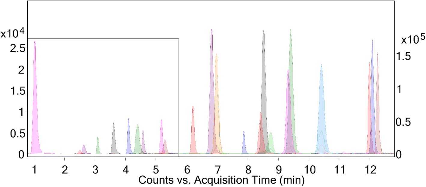Fig. 1 Representative chromatogram of non-derivatized analytes. The time segment from 0 to 5.8 minutes is magnified on a smaller scale (left Y-axis) for better visibility. Retention times for peaks in minutes are as follows: BPS 1.0, BPF 2.5, estriol 2.7, BPE 3.1, BPA 3.6, [¹³C₆]-carbamazepine 3.7, [¹³C₆]-diclofenac 4.1, BPAF 4.4, BPB 4.6, BPC 5.2, estradiol 5.3, ethinylestradiol 5.5, BPAP 6.2, BPZ 6.7, corticosterone 6.8, dienogest 7.0, estrone 7.2, [²H₅]-diazepam 7.9, testosterone and [²H₄]-testosterone 8.4, norethindrone 8.5, tibolone 8.8, BPG 9.1, gestodene 9.3, cyproterone 9.4, norgestrel 10.4, chlormadinone 12.0, drospirenone 12.1, progesterone and [²H₉]-progesterone 12.3.

2.2.2 Instrumental method for derivatized analytes. The method for the derivatized analytes was operated in positive ionization mode and used the optimized parameters of a nebulizer pressure of 15 psi, capillary voltage of +3.5 kV and nozzle voltage of +500 V. The mobile phase flow was 0.625 mL min⁻¹ starting with 25% of solvent A and 75% of solvent B as an isocratic elution for 2.0 min and continued with a gradient elution program as follows: 2.0 to 3.0 min: 75 to 89% B, 3.0 to 5.0 min: 89% B, 5.0 to 7.0 min: 89 to 91% B, 7.0 to 7.5 min: 91% B, 7.5 to 7.6 min: 91 to 99% B, 7.6 to 8.6 min: 99% B, and 8.6 to 8.7 min: 99 to 75% B. The total run time was 9.8 minutes (including reequilibration), out of which the time segment from 2 to 8.8 min was directed to MS, and the rest to waste. A representative chromatogram of derivatized analytes is shown in Fig. 2.

Fig. 2 Representative chromatogram of derivatized analytes. The time segment from 4.8 to 9.8 minutes is magnified on a smaller scale (right Y-axis) for better visibility. Retention times for peaks in minutes are as follows: estriol and [²H₄]-estriol 2.3, ethinylestradiol and [²H₄]-ethinylestradiol 3.5, estradiol and [²H₅]-estradiol 3.6, estrone and [²H₄]-estrone 4.4, BPS 5.0, BPAF 5.6, BPF 6.0, BPE 6.6, BPA and [²H₁₆]-BPA 7.2, BPB 7.7, BPC 7.7, BPG 7.9, BPAP 8.3, and BPZ 8.4.

2.3 SPE extraction procedure

For SPE extraction, a method previously developed in-house was optimized.⁵⁵ Strata X, polymeric reversed phase 60 mg/3 mL SPE cartridges (Phenomenex, Torrance, CA, USA) were used for the SPE extraction. Prior to extraction, the cartridges were preconditioned with 10 mL methanol and 5 mL MQ water. 200 mL of unfiltered surface water samples previously acidified with 1 M HCl to a pH value of 4.0 were loaded onto the cartridges with a vacuum manifold at a constant flow rate of 5 mL min⁻¹. After loading, the cartridges were washed with 5 mL of MQ water and then dried under maximum vacuum for 20 minutes. Elution was performed with 2 mL (four-times 500 μL) of elution solvent (ACN : MeOH = 1 : 1) under slight vacuum into 2 mL microcentrifuge tubes. The eluates were then dried under a gentle stream of nitrogen in a water bath kept at 40 °C. After complete drying, the samples were reconstituted in 200 μL of reconstitution solvent (ACN : MeOH = 3 : 1), vortexed for 1 minute and sonicated in an ultrasonic bath for 15 minutes. After sonication, aliquots of 50 μL of each sample were transferred to 1.5 mL microcentrifuge tubes for derivatization, and the rest of each sample was transferred into vials with inserts, placed into the autosampler and analyzed as non-derivatized samples with LC-MS/MS.

2.4 Derivatization procedure

The 50 μL of each sample taken from the non-derivatized sample as described in Section 2.3 was again quickly dried under a gentle stream of nitrogen in a water bath kept at 40 °C. 50 μL of 100 mM sodium bicarbonate was added to the dried remainder in the tubes which were then vortexed for 1 minute and sonicated in an ultrasonic bath for 15 minutes. After sonication, 50 μL of 1 mg mL⁻¹ of a freshly prepared dansyl chloride solution in acetone was added to each sample. The tubes were then transferred into a previously heated reaction mixer and shaken at 600 rpm at 70 °C for 5 minutes. After this time, the samples were once again dried under a gentle stream of nitrogen in a water bath kept at 40 °C. After complete drying, the samples were reconstituted in 200 μL of reconstitution solvent, vortexed for 1 minute and sonicated in an ultrasonic bath for 15 minutes. After sonication, the tubes were transferred into a previously cooled Eppendorf 5425 R microcentrifuge (Eppendorf, Hamburg, Germany) and centrifuged at 8 °C and 21 300×g for 15 minutes. Lastly, 120 μL of the supernatant was transferred into vials with inserts, placed into the autosampler and analyzed as derivatized samples with LC-MS/MS.

The signal gain obtained by derivatization in comparison with that of non-derivatized samples was evaluated on ten non-zero concentration point calibration curves of derivatized and non-derivatized samples.

2.5 Preparation of samples for validation

Individual standard stock solutions were initially prepared in volumetric flasks with HPLC grade methanol in concentrations ranging from 1 to 4 mg mL⁻¹. A solution of each standard was then appropriately diluted with methanol and added to a different volumetric flask to obtain a combined stock solution of all standards in appropriate concentrations. The concentrations of each analyte in the mix were adjusted roughly to achieve comparable signals. This combined stock solution was then used for the spiking of simulated samples. The same procedure was repeated with each individual isotopically labeled internal standard to obtain a combined solution of internal standards.

The combined solution of standards was used for spiking the samples in 200 mL amber glass volumetric flasks to obtain calibration standards as presented in Table S4.† After acidifying (as described in Section 2.3), each sample (for validation and real samples) was also spiked with 200 μL of a mixture of isotopically labeled internal standards.

Two quality control (QC) samples at low (QC_L) and high concentrations (QC_H) were prepared (in triplicate) in the same manner as described above: a separate combined stock standard solution was spiked into sample flasks to obtain the desired concentrations (Table S4†) which were afterwards spiked with 200 μL of the isotopically labeled internal standard stock solution.

For the determination of validation parameters where different concentrations were required (for LOQ samples and for the utilization of the standard addition principle), two different combined stock solutions were prepared for further spiking, depending on the concentrations needed for each substance in each assay.

2.6 Method validation criteria

The method was validated in terms of linearity, limit of detection (LOD), limit of quantitation (LOQ), method precision and accuracy, recovery, matrix effect (ME), detector specificity and autosampler stability. The validation parameters were leaned on a relevant guideline from the US EPA⁵⁶ and our own criteria based on existing analytical experience in environmental analysis and related fields of bioanalytics.

The linearity was evaluated for each analyte using a combined stock solution, at seven non-zero concentration points, each prepared in duplicate (Table S4†). The correlation coefficient for determining linearity was calculated by using least-square linear regression and each calibration curve was also inspected visually. The determination coefficient acceptance criterion was set at R² > 0.99.

LOQs were determined by evaluating several parameters determined at samples with the lowest possible concentration (at the LOQ value). The parameters were the signal to noise ratio (S/N) > 10 (calculated peak-to-peak based on area with the closest baseline region to the peak with a duration of at least 2 minutes), signal to average blank sample signal (S/B) > 5 (calculated peak-to-peak based on area), accuracy of 50–150% and relative standard deviation (RSD) of less than 50%, each performed on two parallel samples. LODs were calculated as LOQ/3.

The method precision was evaluated in terms of repeatability and reproducibility from measurements performed on the same day (intra-day precision) and three consecutive days (between-day precision) for QC samples (in triplicate) and at each calibrator and sample (in duplicate) on each day, calculated as the RSD. The acceptance criterion was RSD ≤ 20%.⁵⁶ Injection repeatability was evaluated by re-injecting QC samples 10 times. The acceptable values were RSD ≤ 10%.

The method intra-day accuracy was calculated as the ratio of the calculated and theoretical concentrations of analytes at two QC levels and was denoted as a percentage (%). The acceptable values were set in the range of 70–130%.⁵⁶

Recovery was determined by performing an extraction of a spiked MQ solution in triplicate and one calibration curve in MeOH with no extraction. It was calculated by using the following equation: (average slopes of spiked MQ solutions/slope of an equivalent calibrator curve) × 100%. All calibrator slopes used in determining the recovery were composed of seven non-zero concentration points. The recovery was denoted as a percentage (%) and was deemed acceptable for values 50–130%. These limits are preferred, although they can also be lower for specific analytes, if adequate repeatability is achieved.

ME for each respective matrix was determined by performing an extraction of each spiked matrix sample in duplicate and an extraction of a spiked MQ solution in triplicate. It was calculated by using the following equation: ((average slopes of spiked matrix samples/average slopes of equivalent spiked MQ solutions) − 1) × 100%.⁵⁷ All calibration curves used in determining the ME were comprised of seven non-zero concentration points. The values were denoted as a percentage (%) and were expected to fall between ±30%, where 0% means no matrix effect, negative values represent signal suppression and positive values a signal enhancement in comparison with the spiked standard solution, without a matrix.

Detector specificity was determined by observing the ion-channel crosstalk (ICCT). The intensity of signals in samples of each individual analyte with a concentration corresponding to approximately the middle of its respective calibration curve in MRM channels not corresponding to the analyte was examined. The acceptable quotient of the obtained peak area (PA) in other MRM channels and the PA in the analyte MRM channel was ≤0.01% as this represents instrument noise and would prove an insignificant interference even at concentration differences of a factor higher than the method's complete concentration range.

The satisfactory sample stability in relation to method accuracy was deemed acceptable in the range of 70–130%. In the case of our analytes, their long-term stability is suitable, although it should always be determined.^58,59 The requirements for autosampler stability are more stringent, depending on the analytes. It was evaluated on QC samples at 8 °C. Stability is expressed as the ratio of the PA corresponding to a certain time (24 or 48 h) and the PA of the sample at the initial time.

2.7 Sample collection

The glass sampling bottles used for the collection of surface water samples were pre-cleaned in the laboratory with detergent, distilled water, 1 M HCl, 1 M NaOH, 2 M HNO₃ and methanol, consecutively. Sampling was achieved by using a 3 meter retractable telescopic pole obtained from Bürkle (Bad Bellingen, Germany). The sampling bottles were rinsed with surface water at each sampling location three times before sampling, where 1 L of sample was collected at a standardized depth of 1 meter. For method validation purposes, seven samples with different matrices were selected, namely a lake sample, four river samples, a stream, and a channel sample. The locations are presented with coordinates in Table 3. After collection, the samples were placed in a refrigerator (5–8 °C) prior to analysis, which was always performed in less than 72 hours.

At each sampling event, one field blank was also prepared. For this, two of the same sampling bottles were used as for the collection of the real samples. 1 L of MQ water was recurrently transferred between bottles once at each sampling location, simulating the worst-case scenario for sample contamination.

2.8 Surface water sample analysis

After collection, the samples were initially analyzed by our optimized methodology (Sections 2.2 to 2.4) and their concentrations were calculated directly with calibration curves obtained in method validation. As both chromatographic methods are performed on the same column with the same mobile phase, they are run in sequential order. Quantification for analytes suitable for derivatization was performed in both derivatized and non-derivatized samples (both prepared in a single extraction) while for non-derivatized analytes, quantification was performed only in non-derivatized samples. As some overlap exists with both calibrations, all derivatized analytes were quantitated with both methods (except for EE2), as presented in Table S5.† Therefore, analytes which can be derivatized (i.e. BPA) are described in the article as both their non-derivatized forms with unchanged chemical names (i.e. BPA) and derivatized forms with a -D suffix (i.e. BPA-D).

Additionally, to further confirm the method performance, three additional surface water samples were selected for evaluating the method performance with the standard addition (SA) principle. A clean river sample (a few kilometers away from major cities and industries), a burdened river sample (along the banks of a river near a larger town) and a lake sample (a river-based lake in a small town) were collected. All three samples were collected in larger volume (2 L). Based on the measured concentrations of analytes, one separate combined stock solution of standards was prepared with approximately the average of 100, 250 and 500% of the determined concentrations in the real samples. This solution was then used for spiking in a three-point calibration for all three samples. Finally, the analyte's concentration was calculated back from the obtained SA calibration curve for each analyte and compared to the value calculated directly from the method calibration curves.

3. Results and discussion

3.1 Analytical method development

The molecular structures of steroids (and some bisphenols) are very similar (Fig. S1†). Consequently, the formed product ions are often the same (Table S2†). Therefore, ICCT would be very likely if these substances were not separated chromatographically. During method development, most issues with separation were observed for two groups of substances (one being E1, E2, and EE2 and the second drospirenone, gestodene, norethindrone and tibolone). Therefore, to achieve suitable separation, various stationary phases were tested. Different C18 columns were tested, namely: Kinetex C18 50 × 2.1 mm, 2.6 μm; Kinetex XB-C18 100 × 2.1 mm, 2.6 μm (Phenomenex, Torrance, CA, USA); Eclipse XDB-C18 50 × 1.0 mm, 3.5 μm and Poroshell 120 EC-C18 100 × 3.0 mm, 2.7 μm (Agilent Technologies, Santa Clara, CA, USA), a pentafluoro phenyl phase column Kinetex F5 100 × 2.1 mm, 2.6 μm (Phenomenex, Torrance, CA, USA), several phenyl-hexyl (PH) columns, namely: Poroshell 120 PH 50 × 2.1 and 150 × 4.6 mm, both 2.7 μm (Agilent Technologies, Santa Clara, CA, USA) and Acquity CSH PH 100 × 2.1 mm, 1.7 μm (Waters Corporation, Milford, MA, USA), and finally, a bi-phenyl (BP) column. A Kinetex BP 50 × 2.1 mm, 2.6 μm column (Phenomenex, Torrance, CA, USA) has proved to be the column which enabled the best separation of both groups of steroids and bisphenols and was selected for further work. BP columns exhibit strong polar–π and π–π interactions. The former enabled a great difference in the retention of E1, E2 and E3, while the latter enabled the separation of the SH group. All substances with similar masses and the same product ions (Table S2†) were separated adequately after a multi-step development of a complex gradient elution program in a 14 minute run time.

Several different mobile phases such as acetic and formic acid, ammonium acetate, ammonium carbonate, ammonium formate and ammonium fluoride were tested on the separated mixture for signal intensity. The signal intensity of ammonium fluoride was comparably better by at least one order of magnitude, as was also determined by some other researchers.^60–62 A 0.2 mM concentration of ammonium fluoride proved optimal, as lower concentrations showed greater variations in retention times of analytes, and higher concentrations, decreasing signal intensity. In terms of the organic modifier, the use of methanol has enabled signals of a 2- to 10-fold higher intensity than acetonitrile and was therefore selected for further method development.

Since the analytes with the lowest signal intensity in our method were expectedly hydroxy substances (group on position 3) that ionize in negative mode (Table S2†), a derivatization was planned beforehand to obtain suitable sensitivity.⁶³ As the mentioned phenolic hydroxy group is quite reactive, dansyl chloride was selected as the derivatization agent, because an established derivatization procedure which is described as simple, quick, and cheap⁶⁴ was optimized for our purpose (Fig. S2†). Extensive variations of different derivatization parameters were evaluated on selected substances, such as different bases (NaOH and triethylamine), dansyl solvents (MeOH, acetonitrile, and dichloromethane), dansyl concentrations (0.5 to 5 mg mL⁻¹) and different combinations of solvent volumes (from 10 to 1000 μL), temperatures (room temperature to 80 °C) and reaction times (1 minute to a few hours). After roughly estimating parameters based on the analytes' signal gain, a more fine-tuned optimization of different solvent volumes, reaction temperatures and reaction times was evaluated to further improve the signal gain. To improve the accuracy of the determination, this was performed with the comparison of slopes (Fig. S3†) and correlation coefficients of four non-zero concentration point calibration curves instead of just a single sample experiment. On variating the volume of reagents, the differences in reaction efficiencies were mostly negligible, while variations in temperature determined that 70 °C has proven beneficial compared to lower and higher temperatures (especially for E3 and E2). Reaction times shorter and longer than 5 minutes yielded marginally decreasing efficiencies, so a 5 minute reaction time was selected.

All analytes that ionize in negative mode were successfully derivatized (shown in Table S2†). The derivatized analytes obtained one (steroids) to two (bisphenols) dansyl fragments (the signals for mono-derivatized BPs were insignificant in a separate analysis of derivatization efficacy). A gradient elution program was developed for derivatized analytes in a 9.8 minute run time, which proved to be satisfactory in terms of selectivity (Table S3†). As all the water extracts were split into two parts (one for derivatization and one remaining) with the remaining part being chemically unchanged, it was deemed suitable to also analyze the non-derivatized portion of the sample alongside the derivatized one. This both eliminates any issues resulting from derivatization for non-derivatized analytes such as SHs (possibility of degradation due to the heating and alkaline conditions) and also enables the analysis of analytes by both methods to further confirm the accuracy of the method and to enable a much wider concentration range.

Furthermore, no interference from the non-derivatized analytes was observed in the method for derivatized analytes, as they are eluted from the column with a lower percentage of organic modifier than the starting conditions of the derivatized chromatographic method. No other coeluting peaks or other interferences (related to substances that can be derivatized in samples but were not analyzed in the method) were observed.

A signal gain obtained by derivatization compared to that of non-derivatized samples was determined for all the derivatized analytes, at least by a factor of 2 for BPS and to more than 450 for EE2 (Table 1). This is especially important for analytes where the lowest LOQ values are required because of their sub-ng L⁻¹ effective concentrations in the environment (and consequently the requirements by the 2018 EU watchlist), as these values could not be obtained without derivatization.⁶⁵ This is mainly the case for estrogens and EE2 where LOQ values without derivatization are ranging from 2.3 to 40 ng L⁻¹ and are as low as 0.060 to 0.32 ng L⁻¹ after derivatization. A graphical representation of derivatization signal gain on an example of E2 is also presented in Fig. S4.†

Table 1 Derivatization sensitivity improvement by determining the signal gain factor from the comparison of hormone and bisphenol slopes on ten non-zero concentration point calibration curves pre- and post-derivatization. Only analytes that can be derivatized are present in the table

	E3	E2	EE2	E1	BPS	BPF	BPE	BPA	BPAF	BPB	BPC	BPAP	BPZ	BPG
Slope (pre-dansylation)	251	258	139	2005	110 329	4125	844	14 968	10 907	766	4160	1826	7032	148
Slope (post-dansylation)	12 289	34 401	63 127	45 181	266 087	381 586	38 974	349 112	91 137	144 916	247 638	20 004	86 449	3974
Signal gain factor	49	133	453	23	2.4	93	46	23	8.4	189	60	11	12	27

---

3.2. Extraction procedure optimization

Then the extraction procedure was optimized to provide the desired LOQ levels, while maintaining sample manipulation simplicity. Polymeric reversed phase SPE cartridges from different manufacturers were tested, namely Oasis HLB 60 mg/3 mL (Waters Corporation, Milford, MA, USA), Chromabond HR-X 200 mg/3 mL and Chromabond HLB 60 mg/3 mL (both Macherey-Nagel, Düren, Germany) and Strata X 60 mg/3 mL (Phenomenex, Torrance, CA, USA). Strata X has proven to be better than the compared cartridges for our application with both better recovery and precision (Table S6†). Strata X cartridges with a larger sorbent loading (200 mg/6 mL) were also tested, but the recoveries achieved were at best comparable to those with a smaller sorbent loading. Thus, their use was not justified due to the higher price.

The procedure was based on a method previously developed in-house for monitoring other pharmaceuticals in surface waters.⁵⁵ Key parameters important for the sensitivity of the method were tested to assess the optimal loading parameters on spiked MQ samples (Table S7†). At volumes higher than 500 mL, decreasing recovery values for EE2, testosterone and progesterone were observed. Due to the increased loading time of a 500 mL sample and the fact that adequate LOQ values were obtained for most analytes even with 200 mL of sample, method development was continued with the latter volume. Flow rates up to 5 mL min⁻¹ were satisfactory both in terms of recovery and precision and were deemed adequate for further method development, as the parameters were worse with higher flow rates for most analytes.

Ideally, only a small volume of sample would be loaded with a fast flow rate, achieving greater time efficiency, but would prove obtaining low-ng L⁻¹ LOQ levels difficult. On the other hand, large loading volumes and fast loading rates can cause decreased (and inconsistent) recovery,^66,67 as was also observed in our case.

The samples were not pre-filtered before being loaded onto cartridges, as this is not recommended due to the potential loss of analytes bound to particles and should be avoided.⁶⁸ As most methods in the literature filter samples before loading, we deem this to be an important distinction of our method. All samples were loaded in full volume successfully even though partial clogging was observed, which additionally supports the selection of the 200 mL sample loading volume.

3.3 Method validation

Method specificity was confirmed by analyzing samples for potential ICCT between analytes and/or isotopically labeled internal standards. No measurable signals were found for other substances at the corresponding retention times. The ratio between each analyte's quantifier and qualifier ion signal was determined in all samples during the method validation and surface water sampling and was within the acceptable (±20%) range.⁶⁹

The visually inspected linearity of the calibration curves and the high determination coefficients (mostly above 0.999) showed a wide calibrator concentration range ratio for all the analytes (1000), except for BPC, where the range was only 200 (Table 2). Because analytes that have been derivatized (E1, E2, E3, EE2 and bisphenols) can also be quantified non-derivatized, their linearity ranges overlap. As the signal intensities of non-derivatized analytes are relatively low even in the highest points used in the calibration curve (Table S5†) it is possible to combine both calibrations to obtain an even wider monitoring concentration range, for monitoring samples with higher concentrations, such as wastewaters. This is a significant advantage of the method, as it enables even greater utility, if needed.

Table 2 Analytical method validation parameters for both the non-derivatized and derivatized analytes^a

Compound name	Calibration range (ng L^−1)	R ^2	LOD (ng L^−1)	LOQ (ng L^−1)	Accuracy (%)		Intra- and between-day precision (%)		Injection repeatability (%)		Recovery (%)	ME (%)
					QCL	QCH	QCL	QCH	QCL	QCH		DW	RW
a Notes: QCL is the low and QCH the high concentration QC sample. LOD. limit of detection; LOQ, limit of quantitation; ME, matrix effect; DW, drinking water; RW, river water; *, analytes denoted with -D are derivatized with dansyl chloride; /, the signal of the corresponding analyte is too low at the QCL level to be adequately assessed and is therefore relevant at this level only when derivatized.
BPS	0.3–300	0.9998	0.08	0.24	109–112	96–97	1.0/7.7	1.2/5.8	1.4	1.0	99.7	−9.4	−17.8
BPF	4.0–400	0.9995	1.3	4.0	—	97–100	—	1.8/5.4	—	1.4	100.8	9.4	17.4
Estriol	2.3–75	0.9990	0.75	2.3	—	97–99	—	6.2/9.0	—	2.3	89.5	5.9	22.2
BPE	1.5–300	0.9995	0.5	1.5	103–117	93–94	0.3/14.6	2.4/5.6	0.4	1.5	104.4	6.5	24.2
BPA	0.8–300	1.0000	0.28	0.84	—	95–96	—	0.5/7.0	—	0.4	109.8	0.3	17.1
BPAF	1.5–300	0.9981	0.5	1.5	—	90–99	—	1.0/6.6	—	0.7	112.9	−5.8	20.9
BPB	1.5–300	0.9998	0.5	1.5	108–115	97–98	8.9/10.5	3.0/4.8	7.2	2.6	118.0	8.3	16.5
BPC	9.0–300	0.9989	3.0	9.0	—	88–94	—	3.2/6.8	—	2.9	111.3	−12	19.6
Estradiol	40–400	0.9994	13.3	40	—	94–97	—	1.5/5.2	—	1.3	111.2	8.6	19.5
Ethinylestradiol	25–75	0.9992	8.8	26	—	88–95	—	5.2/18.5	—	2.3	88.2	5.2	10.2
BPAP	0.4–300	0.9999	0.14	0.42	100–110	98–101	2.0/8.0	1.9/5.9	2.2	1.5	103.8	−3.6	6.1
BPZ	2.0–200	0.9999	0.67	2.0	—	101–102	—	1.5/7.5	—	1.5	100.0	−5.5	0.6
Corticosterone	0.9–850	0.9998	0.23	0.68	81–82	109–110	4.4/7.3	1.0/7.8	1.8	0.7	88.9	5.1	−13.4
Dienogest	0.4–400	1.0000	0.11	0.32	90–92	106–107	2.3/4.9	1.4/5.8	1.9	1.0	89.1	−8	−20.6
Estrone	3.0–30	0.9999	1.0	3.0	—	98–102	—	3.2/5.6	—	2.5	98.8	−1.3	21.0
Testosterone	0.1–100	1.0000	0.046	0.14	96–97	101–102	2.1/6.6	1.3/2.8	1.4	1.1	99.2	−3.3	1.7
Norethindrone	0.8–750	0.9994	0.20	0.60	114–115	95–98	1.5/5.3	0.4/4.3	0.5	0.6	99.9	−4.6	5.8
Tibolone	2.0–700	0.9976	0.65	2.0	73–75	113–117	3.1/9.2	0.4/3.9	2.9	0.4	96.4	6	10.7
BPG	6.0–600	0.9994	2.0	6.0	—	95–98	—	1.5/6.8	—	1.4	97.4	−17.6	14.0
Gestodene	0.55–550	0.9999	0.15	0.44	88–91	104–105	0.6/3.9	0.7/3.3	0.5	0.5	101.4	−3.1	8.3
Cyproterone	1.25–1250	0.9986	0.33	1.0	71–72	109–110	1.7/4.5	1.0/2.5	1.4	1.1	102.4	2.8	8.5
Norgestrel	0.5–500	0.9998	0.13	0.4	106–109	98–100	1.3/3.2	1.1/3.0	0.8	0.8	104.9	−5.6	13.0
Chlormadinone	3.5–3500	0.9998	0.93	2.8	106–106	100–102	1.9/4.5	1.0/7.9	1.9	0.9	93.6	−2.4	12.3
Drospirenone	0.4–400	0.9998	0.11	0.32	106–106	99–102	2.1/4.1	1.6/7.3	2.0	1.3	100.4	−7.6	6.5
Progesterone	0.1–100	0.9997	0.027	0.080	102–108	97–102	3.8/5.4	2.3/6.1	1.0	2.0	94.6	−7.9	−0.6
Estriol-D*	0.075–26	0.9999	0.02	0.06	92–99	101–103	4.9/8.0	3.5/4.0	2.4	0.8	100.3	−5.3	0.5
Ethinylestradiol-D	0.075–26	10 000	0.02	0.06	93–94	100–102	2.8/3.9	2.4/3.5	1.2	0.8	97.1	−2.1	23.4
Estradiol-D	0.4–140	0.9999	0.11	0.32	103–108	98–102	3.0/5.1	0.9/3.2	0.6	0.7	100.9	−10.5	−5.4
Estrone-D	0.03–11	0.9999	0.028	0.084	86–91	100–103	1.6/4.2	3.2/4.8	1.2	1.0	94.6	6.2	13.7
BPS-D	0.3–105	1.0000	0.08	0.24	99–103	102–103	1.0/5.5	1.3/5.9	1.3	0.5	102.0	−1.8	−12.1
BPAF-D	0.3–105	0.9995	0.08	0.24	98–101	99–103	5.1/17.4	2.9/6.9	0.9	0.5	87.3	9.7	−8.4
BPF-D	0.4–140	10 000	0.11	0.32	97–107	100–104	2.3/7.7	3.1/5.2	1.4	0.7	88.2	−8.9	2.5
BPE-D	0.3–105	10 000	0.08	0.24	97–100	98–101	3.2/6.9	0.3/4.2	1.0	0.8	98.3	−4.8	4.4
BPA-D	0.3–105	10 000	0.08	0.24	93–117	98–99	0.5/15.6	0.9/5.4	0.3	0.7	97.7	−4.0	−1.8
BPB-D	0.3–105	0.9999	0.08	0.24	99–100	99–100	2.1/6.5	2.3/4.8	0.8	0.6	87.6	0.0	1.8
BPC-D	1.5–105	0.9997	0.5	1.5	87–105	96–98	8.5/18.4	1.2/7.5	2.6	1.1	73.0	−10.1	20.2
BPG-D	0.6–210	1.0000	0.16	0.48	91–108	100–102	6.1/16.0	1.3/17.3	2.9	1.1	80.5	−17.1	22.7
BPAP-D	0.3–105	0.9997	0.08	0.24	89–89	94–97	7.5/9.2	3.0/6.9	2.6	0.6	77.0	9.9	−9.6
BPZ-D	0.2–70	0.9999	0.053	0.16	90–90	93–97	7.8/9.1	1.5/4.2	2.1	1.0	79.6	1.7	−2.8

---

Our assessment of acceptable LOQ values was based on S/N, S/B, accuracy, and precision at the representative concentration (Table S8†). The S/B and accuracy parameters are based on the EPA guideline, with additional stringent requirements based on existing analytical experience in related fields of environmental and bioanalytical studies. The representative chromatograms used in calculations of S/N values for each analyte are shown in Fig. S5† (non-derivatized) and Fig. S6† (derivatized). The LOQ values of most analytes are limited by the S/N value, while some analytes have shown some level of background contamination at relatively high S/N values. This was the case for BPA (S/B ratio over 5 and S/N ratio > 1800), and to a lesser extent also for some other bisphenols (BPS, BPZ and BPAF). Calculating LOQ values simply from S/N would therefore deem much lower values which proves that adding additional S/B requirements was needed for obtaining relevant LOQ values.

Some published methods report only estimates of theoretically achievable LOQ values, by calculation from the S/N ratios obtained at much higher concentration levels.^10,70–72 This is not a good practice, as in this way, the performance of the method can be artificially improved but may not be representative of the true sensitivity.²⁵ Therefore, in our study, the LOQ values were determined at the relevant concentrations (the samples with the same concentrations as the LOQ values). Furthermore, it is also important that the results are reliable in terms of the acceptable accuracy and repeatability proposed, as many measurements in the environment are close to these values.

The LOQ values for all analytes were in the sub-ng L⁻¹ range (Table 2), as was the aim of the study (with the exception of tibolone, chlormadinone and BPC). The lowest values were obtained for E3 and EE2, even as low as 0.060 ng L⁻¹. The acceptable method detection limit for EE2 is 0.035 ng L⁻¹ in the 2018 EU watchlist (Vella, 2018) and is therefore easily achieved with our method (LOD = 0.020 ng L⁻¹). Furthermore, the LOQ values in our method were not extrapolated but determined in actual samples with sub-ng L⁻¹ concentrations, and were obtained with 200 mL of sample loaded, and considering the fact that method development has proven volumes up to 500 mL acceptable in terms of recoveries, the acceptable limit could easily be set even lower.

The developed method was accurate on both QC levels, as the results are well within the proposed levels. Most of the values fall in an even stricter range of 90–110% which further underlines the accuracy of the method (Table 2).

The results for intra- and between-day precisions are also within the proposed limits of RSD ≤ 20%, while values for injection repeatability were well within the limits with most values below 3%. Altogether, this verifies the precision of the method (Table 2).

SPE recoveries were all in the 50–130% range, with most values close to 100%.

All the ME values were in the ±30% range (Table 2). The MEs in drinking water (obtained from the tap in-house) and river water (obtained as a composite grab sample from the Drava River, located in a sparsely populated area about 5 km downstream from a major city) were low, mostly due to the inclusion of isotopically labeled internal standards in the method, especially in river water. The ME effect could also be tested by spiking the empty matrix samples after extraction, but we have chosen to spike before it as it is difficult to obtain an environmental matrix without any trace of analytes. We believe this is advantageous, as the ME encompasses the total effect of the matrix on the instrument signal (i.e., both the matrix effect on recovery and the ion suppression on the MS system). The comparison of matrix effects with and without the use of internal standards is presented in Table S9.†

All analytes were found to be stable over 24 and 48 hours in the autosampler at 8 °C where the loss of signal was <10% for most analytes, except for BPZ where the loss is 15%, and E1, with slightly over 20% signal loss at both QC levels (Table S10†). Both analytes have shown better stability in their derivatized form, so this was deemed acceptable, as they are primarily determined as derivatized. Sample stability is an important factor and was deemed acceptable for all analytes for at least 48 hours, especially as the combined analysis times for a larger number of samples can extend for longer periods of time. This was also valid for the derivatized analytes, as the derivates were suitably stable and did not convert back into their non-derivatized form.

3.3.1 Standard addition principle. To further evaluate the accuracy of the measured concentrations, a standard addition (SA) experiment was performed for evaluating the relative matrix effect in samples. Such an addition was performed on a set of three different samples as described in Section 2.8. The samples were purposely selected as three significantly different surface water matrices, to cover a wide selection of possible samples. The concentrations determined by both methods are presented in Table S11.† The results from the SA calculations are mostly within ±10% (with only a few measurements within ±20%) of the value calculated from the method's calibration curves. Therefore, we can conclude that the developed method calibrated in MQ gives adequately accurate and precise results without the need for sample fortification. Even though the EPA 539 method recommends running a fortified sample with each analysis batch, it seems that in the literature this is usually not the case^10,23,24,32 as the standard addition principle is very time consuming. Similar to our methodology, in most methods in the literature, the SA principle is used solely to confirm that the method calibration is adequate in different matrices and is not used in routine analysis.

3.4 Method application: surface water samples

The method was applied to a representative selection of seven surface water samples with different matrices, namely one lake sample (LK), four river samples (R1, R2, R3, and R4), one stream (ST) and one channel sample (CH) to determine the occurrence of EDs and their concentration levels. The results from the measurements are shown in Table 3. In the field blank sample most analytes were not detected, except for BPA (both methods), estrone and BPS (method for derivatized analytes), where the values were below the LOQ. Even with very low LOQ values achieved by the method, the analytes' concentrations in most samples were determined below LOQ levels or were not detected. With the method for non-derivatized analytes, BPS and BPA were quantified in 6 of the 7 samples. The determined concentrations are quite expected, given the widespread persistence of BPA and the use of BPS as its substitute.^73–75 Among SHs, dienogest, norgestrel, chlormadinone and drospirenone were present in quantifiable concentrations in at least one sample (4.6 to 38 ng L⁻¹). This demonstrates the importance of their evaluation in the environment, because even though they were not quantified in many samples, the measured concentrations are relatively high, exceeding safe concentrations (i.e. 0.19 ng L⁻¹ for norethindrone). Progesterone (6 samples) and estrone (3 samples) were the only NHs quantified in samples without derivatization.

Table 3 Concentrations of analytes measured in representative surface water samples^a

Sample name	LK	R1	R2	R3	R4	ST	CH
Latitude	46.440431 N	46.459027 N	46.516857 N	46.527754 N	46.543028 N	46.465591 N	46.461673 N
Longitude	15.680078 E	15.752519 E	15.699987 E	15.712321 E	15.703320 E	15.657304 E	15.670147 E
a Notes: n.d., analyte not detected; <LOQ, measurement under the method quantitation limit;*, analytes denoted with -D are derivatized with dansyl chloride.
Measured concentrations (ng L^−1)
BPS	n.d.	3.7 ± 0.1	4.0 ± 0.1	4.0 ± 0.2	3.6 ± 0.2	28 ± 1	7.0 ± 0.1
BPF	n.d.	n.d.	n.d.	n.d.	n.d.	<LOQ	n.d.
Estriol	n.d.	n.d.	n.d.	n.d.	n.d.	<LOQ	n.d.
BPE	n.d.	n.d.	n.d.	n.d.	n.d.	n.d.	n.d.
BPA	<LOQ	4.9 ± 0.2	4.7 ± 0.4	3.0 ± 0.4	5.2 ± 1.2	47 ± 7	5.0 ± 0.6
BPAF	n.d.	n.d.	n.d.	n.d.	n.d.	n.d.	n.d.
BPB	n.d.	n.d.	n.d.	n.d.	n.d.	n.d.	n.d.
BPC	n.d.	n.d.	n.d.	n.d.	n.d.	n.d.	n.d.
Estradiol	n.d.	n.d.	n.d.	n.d.	n.d.	n.d.	n.d.
Ethinylestradiol	n.d.	n.d.	n.d.	n.d.	n.d.	n.d.	n.d.
BPAP	n.d.	n.d.	n.d.	n.d.	n.d.	n.d.	n.d.
BPZ	n.d.	n.d.	n.d.	n.d.	n.d.	n.d.	n.d.
Corticosterone	n.d.	<LOQ	n.d.	<LOQ	<LOQ	n.d.	<LOQ
Dienogest	<LOQ	n.d.	n.d.	n.d.	n.d.	4.6 ± 0.2	n.d.
Estrone	3.8 ± 0.4	n.d.	n.d.	n.d.	n.d.	46 ± 4	5.8 ± 0.4
Testosterone	n.d.	n.d.	n.d.	n.d.	n.d.	n.d.	n.d.
Norethindrone	n.d.	<LOQ	n.d.	n.d.	<LOQ	n.d.	n.d.
Tibolone	n.d.	n.d.	n.d.	n.d.	n.d.	n.d.	n.d.
BPG	n.d.	n.d.	n.d.	n.d.	n.d.	n.d.	n.d.
Gestodene	n.d.	n.d.	<LOQ	n.d.	<LOQ	n.d.	n.d.
Cyproterone	<LOQ	<LOQ	<LOQ	<LOQ	<LOQ	n.d.	<LOQ
Norgestrel	<LOQ	<LOQ	<LOQ	<LOQ	<LOQ	12 ± 0	38 ± 3
Chlormadinone	<LOQ	12 ± 0	<LOQ	n.d.	<LOQ	n.d.	n.d.
Drospirenone	n.d.	9.0 ± 0.1	n.d.	n.d.	<LOQ	n.d.	n.d.
Progesterone	2.8 ± 0.1	2.2 ± 0.0	<LOQ	2.2 ± 0.0	2.8 ± 0.1	6.0 ± 0.1	3.0 ± 0.1
Estriol-D*	0.14 ± 0.05	n.d.	n.d.	n.d.	n.d.	1.8 ± 0.1	0.51 ± 0.02
Ethinylestradiol-D	n.d.	0.06 ± 0.06	n.d.	n.d.	<LOQ	0.23 ± 0.06	0.23 ± 0.00
Estradiol-D	n.d.	<LOQ	n.d.	n.d.	n.d.	2.1 ± 0.1	<LOQ
Estrone-D	3.7 ± 0.1	0.49 ± 0.05	0.43 ± 0.05	0.58 ± 0.04	0.52 ± 0.03	50 ± 1	6.0 ± 0.1
BPS-D	<LOQ	3.2 ± 0.2	4.1 ± 0.1	3.5 ± 0.1	3.8 ± 0.0	24 ± 2	7.1 ± 0.5
BPAF-D	n.d.	0.41 ± 0.24	<LOQ	<LOQ	n.d.	<LOQ	<LOQ
BPF-D	<LOQ	<LOQ	<LOQ	<LOQ	<LOQ	2.0 ± 0.2	0.33 ± 0.03
BPE-D	<LOQ	n.d.	n.d.	n.d.	n.d.	<LOQ	n.d.
BPA-D	<LOQ	5.1 ± 0.1	4.6 ± 0.3	2.7 ± 0.1	5.5 ± 0.9	46 ± 6	5.4 ± 1.6
BPB-D	n.d.	n.d.	n.d.	n.d.	n.d.	n.d.	n.d.
BPC-D	<LOQ	<LOQ	<LOQ	<LOQ	<LOQ	<LOQ	<LOQ
BPG-D	n.d.	<LOQ	<LOQ	n.d.	n.d.	n.d.	n.d.
BPAP-D	<LOQ	n.d.	n.d.	n.d.	n.d.	<LOQ	n.d.
BPZ-D	<LOQ	<LOQ	<LOQ	<LOQ	<LOQ	<LOQ	<LOQ

---

The sensitivity of the method for derivatized analytes is higher. Therefore, with lower LOQ values, more analytes are present in samples in quantifiable concentrations, which further underlines the benefit of derivatization. Among natural hormones, E3, EE2, E2 and E1 are all quantifiable in at least one sample, where the concentrations are usually the highest by (at least) one order of magnitude in the stream sample, compared to in other samples (Fig. 3 for non-derivatized analytes and Fig. 4 for derivatized analytes).

Fig. 3 A combined MRM chromatogram of a stream sample, non-derivatized. Only the peaks of analytes present in levels above LOQ values are presented. Retention times for peaks in minutes are as follows: BPS 1.0, BPA 3.6, dienogest 7.0, estrone 7.2, norgestrel 10.4, and progesterone 12.3.

Fig. 4 A combined MRM chromatogram of a stream sample, derivatized. Only the peaks of analytes present in levels above LOQ values are presented. Retention times for peaks in minutes are as follows: estriol 2.3, ethinylestradiol 3.4, estradiol 3.6, estrone 4.4, BPS 5.1, BPF 6.1 and BPA 7.2.

However, it should be noted that it is impossible to evaluate the general state of any watershed included in the study from just one sample, as more sampling events would be needed for proper evaluation. The noticeably highest measured concentrations of estrogens for E1 and E3 are expected as they are both metabolites of E2 and are excreted by humans into the environment.⁷⁶ Among bisphenols, alongside BPS and BPA which are present in measurable concentrations already in the non-derivatized samples, BPAF and BPF are also detectable in quantifiable concentrations with the derivatized method. The sensitivity of the derivatized method is especially important for E1, E2, and EE2, as their environmentally toxic concentrations are ranging from 3 to 74 pg L⁻¹ and also for E3, BPA and BPS (0.47 to 1.0 ng L⁻¹).³⁵ This shows that all the determined concentrations in samples (except one for E3), are higher than their representative safe values. This further underlines the need for the accurate ultra-trace level determination the method facilitates, and consequently enables a much more accurate risk assessment of the watersheds, as even the sub-ng L⁻¹ presence of these substances can now be adequately quantified.

As some analytes are quantifiable by both methods, the determined concentrations can be compared. Such an assessment is possible for BPA and BPS in all samples. All the determined values are comparable (all fall in the ±20% range, with most less than ±10%), highlighting that both calibrations are comparable and useable at the same time, although in different concentration ranges. Estrone, however, was determined in a quantifiable concentration with the method for non-derivatized analytes only in three samples, two slightly above the LOQ and the other with a much higher concentration (all comparable in the ±10% range), while being above the LOQ in all seven samples with the method for derivatized analytes. This further underlines the applicability of the method including derivatization, as it enables higher sensitivity for quantification in ultra-trace levels of analytes, without sacrificing the method performance for non-derivatized analytes.

3.5 Method comparison and utility

The proposed method has been proven to be useful in a wide concentration range and with environmentally relevant LOQ values for a broad selection of analytes. The published methods show considerably varied principles of method validation and obtained LOQ values, thus making it almost impossible to compare the methodologies used (Table S1†). Most methods only measure the concentrations of a smaller number (up to 10) of hormonal or bisphenol analytes with LOQ values in the sub-ng L⁻¹ to ng L⁻¹ range while usually not describing either how or at what concentrations these values were obtained. Even though several methods by other authors achieve comparable LOQ values to ours,^41,71,77,78 they were either calculated from higher concentration samples and extrapolated to S/N values of 10 (or not described), most commonly below the methods' linearity range by at least a few orders of magnitude. Therefore, only a handful of methods are comparable with sub-ng L⁻¹ LOQ values and linearity ranges spanning in the same range with comparable sample preparation and analysis times. However, all these methods have extrapolated LOQ values with either a very high concentration from which this value was calculated (5 ng L⁻¹)⁷⁰ and combined chromatographic runs where a mobile phase change is necessary,⁷¹ a complicated sample preparation (prewash twice, condition, load, rinse, wash, dry, elute, change cartridge, condition, combine cartridges, elute, dry, and reconstitute),⁴⁵ or a limited selection of analytes (only 4 NHs).⁷⁷ Therefore, we believe our method is a clear improvement on all existing methods as it alleviates the shortcomings of each of the mentioned methods in just one simple methodology.

We believe that it is crucial that the quantitation method performs accurately and precisely in the sub-ng L⁻¹ to low-ng L⁻¹ range since this is exactly the region where the safety limits are currently set for most high-priority EDs. This is also the concentration range that is frequently observed in environmental samples in our region. It is therefore essential that the LOQ values are set correctly and low enough for establishing any meaningful assessment of the toxicological burden imposed by the measured EDs. This is the case for many measured analytes in similar studies from similar watersheds as our study, such as the tributaries of the Danube and other rivers in central Europe. The reported concentrations for estrone, estradiol and estriol were ranging from below theoretically calculated LOD values (the lowest being 0.44 ng L⁻¹),^79,80 to below the LOQ (0.08 to 0.31 ng L⁻¹) up to low-ng L⁻¹ values.^24,81,82 In the mentioned studies, ethinylestradiol was only found in concentrations below LOD or LOQ values (0.08 to 3 ng L⁻¹).

This is the same order of magnitude or higher as its potentially toxic concentrations (from 3 pg L⁻¹ to 0.47 ng L⁻¹ for NHs).³⁵ The existing methodology therefore does not enable accurate determination of such low concentrations and does not provide an accurate risk assessment of watersheds (concentrations under high LOD values are reported as zero and those under LOQ values usually as LOQ/2). On the other hand, our method provides clear improvement with reliable results even in such low ranges, further confirmed by a standard addition experiment, which can greatly improve the determination of the waters' burden with both NHs, SHs and BPS at the same time.

Our methodology is therefore useful for monitoring the quality of surface waters, according to the 2018 EU directive, which is important, as the data on the environmental presence of the analytes are still insufficient,²⁰ and a contaminant candidate list from the US EPA (US EPA, 2018).⁸³ As the method was also validated in a drinking water matrix with adequate sub-ng L⁻¹ LOQ values, it is also suitable for the monitoring of drinking water pollutants such as estradiol and BPA.^84,85 Furthermore, the method was already successfully used for the analysis of large sample batches from an international project in Central Europe, boDEREC-CE (data not published yet).

4. Conclusion

The aim of this study was to develop an analytical methodology suitable for the monitoring of environmental concentrations of 25 hormones and bisphenols in surface water samples. The developed methodology was based on a simple SPE extraction, where each extracted sample was analyzed with two sequential LC-MS/MS methods using the same analytical column and mobile phase with similar MS settings and was fully validated in terms of selectivity, linearity, limits of quantitation, accuracy, precision, recovery, matrix effect, and stability. The ultra-trace level limits of quantitation were experimentally confirmed by a multivariate approach including signal/noise and signal/blank calculations in samples with sub-ng L⁻¹ concentrations and were not extrapolated from higher concentration samples. The values were achieved with a robust dansyl chloride derivatization which improved signal intensity for all analytes that can be derivatized by a factor of 2 to 450, as most of these analytes ionize insufficiently without it. This enabled achieving environmentally relevant LOQ values with a relatively simple methodology with the least amount of sample manipulation necessary utilizing a mid-ranged LC-MS/MS system for a wide selection of analytes, which represents an important economic improvement over existing methods. Additionally, the method has been proven to be robust in terms of a very low matrix effect in different environmental matrices, which was further confirmed with a standard addition experiment.

The method's suitability for routine application in ultra-trace level quantification was confirmed by analysis of seven representative samples, i.e. one lake, four river, one stream, and one channel sample where twenty-one analytes were detected, and thirteen out of those were quantified in at least one sample. The method's simple sample preparation combined with a wide linear range and robustly determined environmentally relevant LOQ values as low as 60 pg L⁻¹ exceed regulatory requirements (i.e. for ethinylestradiol). Altogether, the method provides a reliable tool for the routine monitoring of 25 important endocrine disruptors in order to provide detailed information on their presence in the environment.

Funding

This research was financially supported by the Slovenian Research Agency (ARRS) grant [P1-0189].

Author contributions

Andrej Grobin: conceptualization, methodology, validation, formal analysis, investigation, data curation, writing – original draft, writing – review & editing, visualization. Robert Roškar: conceptualization, methodology, resources, writing – review & editing, supervision, project administration. Jurij Trontelj: conceptualization, methodology, resources, writing – review & editing, supervision, project administration.

Conflicts of interest

The authors declare no competing interests.

References

1. T. J. Runnalls, N. Beresford, E. Losty, A. P. Scott and J. P. Sumpter, Several synthetic progestins with different potencies adversely affect reproduction of fish, Environ. Sci. Technol., 2013, 47, 2077–2084.
2. P. F. Siegenthaler, P. Bain, F. Riva and K. Fent, Effects of antiandrogenic progestins, chlormadinone and cyproterone acetate, and the estrogen 17α-ethinylestradiol (EE2), and their mixtures: transactivation with human and rainbowfish hormone receptors and transcriptional effects in zebrafish (Danio rerio) eleuthero-embryos, Aquat. Toxicol., 2017, 182, 142–162.
3. V. Delfosse, M. Grimaldi, J.-L. Pons, A. Boulahtouf, A. le Maire, V. Cavailles, G. Labesse, W. Bourguet and P. Balaguer, Structural and mechanistic insights into bisphenols action provide guidelines for risk assessment and discovery of bisphenol A substitutes, Proc. Natl. Acad. Sci. U. S. A., 2012, 109, 14930–14935.
4. D. Mackay, D. M. Hughes, M. L. Romano and M. Bonnell, The role of persistence in chemical evaluations, Integr. Environ. Assess. Manage., 2014, 10, 588–594.
5. J. Corrales, L. A. Kristofco, W. B. Steele, B. S. Yates, C. S. Breed, E. S. Williams and B. W. Brooks, Global assessment of bisphenol A in the environment: review and analysis of its occurrence and bioaccumulation, Dose-Response, 2015, 13, 1559325815598308.
6. A. V. B. Reddy, M. Moniruzzaman and T. M. Aminabhavi, Polychlorinated biphenyls (PCBs) in the environment: recent updates on sampling, pretreatment, cleanup technologies and their analysis, Chem. Eng. J., 2019, 358, 1186–1207.
7. E. Carraro, S. Bonetta and S. Bonetta, in Hospital Wastewaters: Characteristics, Management, Treatment and Environmental Risks, ed. P. Verlicchi, Springer International Publishing, Cham, 2018, pp. 1–16.
8. E. Felis, J. Kalka, A. Sochacki, K. Kowalska, S. Bajkacz, M. Harnisz and E. Korzeniewska, Antimicrobial pharmaceuticals in the aquatic environment - occurrence and environmental implications, Eur. J. Pharmacol., 2020, 866, 172813.
9. C. Gadipelly, A. Pérez-González, G. D. Yadav, I. Ortiz, R. Ibáñez, V. K. Rathod and K. V. Marathe, Pharmaceutical industry wastewater: review of the technologies for water treatment and reuse, Ind. Eng. Chem. Res., 2014, 53, 11571–11592.
10. Z. Huang, J.-L. Zhao, Y.-Y. Yang, Y.-W. Jia, Q.-Q. Zhang, C.-E. Chen, Y.-S. Liu, B. Yang, L. Xie and G.-G. Ying, Occurrence, mass loads and risks of bisphenol analogues in the pearl river delta region, South China: urban rainfall runoff as a potential source for receiving rivers, Environ. Pollut., 2020, 263, 114361.
11. Z. Xu, Y. Jiang, S. H. Te, Y. He and K. Y. Gin, The effects of antibiotics on microbial community composition in an estuary reservoir during spring and summer seasons, Water, 2018, 10(2), 154.
12. L. Gunnarsson, J. R. Snape, B. Verbruggen, S. F. Owen, E. Kristiansson, L. Margiotta-Casaluci, T. Österlund, K. Hutchinson, D. Leverett, B. Marks and C. R. Tyler, Pharmacology beyond the patient – The environmental risks of human drugs, Environ. Int., 2019, 129, 320–332.
13. H. B. Patisaul and H. B. Adewale, Long-term effects of environmental endocrine disruptors on reproductive physiology and behavior, Front. Behav. Neurosci., 2009, 3, 10.
14. E. K. Richmond, M. R. Grace, J. J. Kelly, A. J. Reisinger, E. J. Rosi and D. M. Walters, Pharmaceuticals and personal care products (PPCPs) are ecological disrupting compounds (EcoDC), Elem. Sci. Anth., 2017, 5, 66.
15. M. L. Y. Wan, V. A. Co and H. El-Nezami, Endocrine disrupting chemicals and breast cancer: a systematic review of epidemiological studies, Crit. Rev. Food Sci. Nutr., 2022, 62, 6549–6576.
16. C. Pironti, M. Ricciardi, A. Proto, P. M. Bianco, L. Montano and O. Motta, Endocrine-disrupting compounds: an overview on their occurrence in the aquatic environment and human exposure, Water, 2021, 13, 1347.
17. F. Toner, G. Allan, S. S. Dimond, J. M. Waechter and D. Beyer, In vitro percutaneous absorption and metabolism of Bisphenol A (BPA) through fresh human skin, Toxicol. In Vitro, 2018, 47, 147–155.
18. S. Rattan, C. Zhou, C. Chiang, S. Mahalingam, E. Brehm and J. A. Flaws, Exposure to endocrine disruptors during adulthood: consequences for female fertility, J. Endocrinol., 2017, 233, R109–R129.
19. B. Vessa, B. Perlman, P. G. McGovern and S. S. Morelli, Endocrine disruptors and female fertility: a review of pesticide and plasticizer effects, F&S Rep., 2022, 3, 86–90.
20. K. Vella, Commission Implementing Decision (EU) 2018/840 of 5 June 2018 Establishing a Watch List of Substances for Union-wide Monitoring in the Field of Water Policy Pursuant to Directive 2008/105/EC of the European Parliament and of the Council and Repealing Commission Implementing Decision (EU) 2015/495 (Notified under Document C(2018) 3362), 2018, vol. 141.
21. V. Sinkevičius, Commission Implementing Decision (EU) 2020/1161 of 4 August 2020 Establishing a Watch List of Substances for Union-wide Monitoring in the Field of Water Policy Pursuant to Directive 2008/105/EC of the European Parliament and of the Council (Notified under Document Number C(2020) 5205) (Text with EEA Relevance), 2020, vol. 257.
22. F. Merlo, A. Speltini, F. Maraschi, M. Sturini and A. Profumo, HPLC-MS/MS multiclass determination of steroid hormones in environmental waters after preconcentration on the carbonaceous sorbent HA-C@silica, Arab. J. Chem., 2020, 13, 4673–4680.
23. A. Rico, A. Arenas-Sánchez, C. Alonso-Alonso, I. López-Heras, L. Nozal, D. Rivas-Tabares and M. Vighi, Identification of contaminants of concern in the upper Tagus river basin (central Spain). Part 1: screening, quantitative analysis and comparison of sampling methods, Sci. Total Environ., 2019, 666, 1058–1070.
24. M. Čelić, B. D. Škrbić, S. Insa, J. Živančev, M. Gros and M. Petrović, Occurrence and assessment of environmental risks of endocrine disrupting compounds in drinking, surface and wastewaters in Serbia, Environ. Pollut., 2020, 114344.
25. K. Goeury, S. Vo Duy, G. Munoz, M. Prévost and S. Sauvé, Analysis of Environmental protection agency priority endocrine disruptor hormones and bisphenol A in tap, surface and wastewater by online concentration liquid chromatography tandem mass spectrometry, J. Chromatogr. A, 2019, 1591, 87–98.
26. M. Sun, Y. Bu, X. Xin and J. Feng, Polyurethane functionalized silica aerogel for in-tube solid-phase microextraction of estrogens prior to high performance liquid chromatography detection, Microchem. J., 2022, 181, 107699.
27. A. B. Kanu, Recent developments in sample preparation techniques combined with high-performance liquid chromatography: a critical review, J. Chromatogr. A, 2021, 1654, 462444.
28. P. Šauer, A. Stará, O. Golovko, O. Valentová, A. Bořík, R. Grabic and H. K. Kroupová, Two synthetic progestins and natural progesterone are responsible for most of the progestagenic activities in municipal wastewater treatment plant effluents in the Czech and Slovak republics, Water Res., 2018, 137, 64–71.
29. A. Weizel, M. P. Schlüsener, G. Dierkes and T. A. Ternes, Occurrence of glucocorticoids, mineralocorticoids, and progestogens in various treated wastewater, rivers, and streams, Environ. Sci. Technol., 2018, 52, 5296–5307.
30. V. Kumar, A. C. Johnson, A. Trubiroha, J. Tumová, M. Ihara, R. Grabic, W. Kloas, H. Tanaka and H. K. Kroupová, The challenge presented by progestins in ecotoxicological research: a critical review, Environ. Sci. Technol., 2015, 49, 2625–2638.
31. M. J. Rocha and E. Rocha, Synthetic progestins in waste and surface waters: concentrations, impacts and ecological risk, Toxics, 2022, 10, 163.
32. C. Zheng, J. Liu, J. Ren, J. Shen, J. Fan, R. Xi, W. Chen and Q. Chen, Occurrence, distribution and ecological risk of bisphenol analogues in the surface water from a water diversion project in Nanjing, China, Int. J. Environ. Res. Public Health, 2019, 16, 3296.
33. C. Huang, L.-H. Wu, G.-Q. Liu, L. Shi and Y. Guo, Occurrence and ecological risk assessment of eight endocrine-disrupting chemicals in urban river water and sediments of South China, Arch. Environ. Contam. Toxicol., 2018, 75, 224–235.
34. Z. Wang, J. Yu, J. Yao, L. Wu, H. Xiao, J. Wang and R. Gao, Simultaneous identification and quantification of bisphenol A and 12 bisphenol analogues in environmental samples using precolumn derivatization and ultra high performance liquid chromatography with tandem mass spectrometry, J. Sep. Sci., 2018, 41, 2269–2278.
35. A. Grobin, R. Roškar and J. Trontelj, Multi-parameter risk assessment of forty-one selected substances with endocrine disruptive properties in surface waters worldwide, Chemosphere, 2022, 287, 132195.
36. E. Drakvik, R. Altenburger, Y. Aoki, T. Backhaus, T. Bahadori, R. Barouki, W. Brack, M. T. D. Cronin, B. Demeneix, S. Hougaard Bennekou, J. van Klaveren, C. Kneuer, M. Kolossa-Gehring, E. Lebret, L. Posthuma, L. Reiber, C. Rider, J. Rüegg, G. Testa, B. van der Burg, H. van der Voet, A. M. Warhurst, B. van de Water, K. Yamazaki, M. Öberg and Å. Bergman, Statement on advancing the assessment of chemical mixtures and their risks for human health and the environment, Environ. Int., 2020, 134, 105267.
37. C. Park, H. Song, J. Choi, S. Sim, H. Kojima, J. Park, M. Iida and Y. Lee, The mixture effects of bisphenol derivatives on estrogen receptor and androgen receptor, Environ. Pollut., 2020, 260, 114036.
38. L. Posthuma, R. Altenburger, T. Backhaus, A. Kortenkamp, C. Müller, A. Focks, D. de Zwart and W. Brack, Improved component-based methods for mixture risk assessment are key to characterize complex chemical pollution in surface waters, Environ. Sci. Eur., 2019, 31, 70.
39. A. Booth, D. S. Aga and A. L. Wester, Retrospective analysis of the global antibiotic residues that exceed the predicted no effect concentration for antimicrobial resistance in various environmental matrices, Environ. Int., 2020, 141, 105796.
40. M. Ashfaq, Q. Sun, C. Ma, A. Rashid, Y. Li, S. I. Mulla and C.-P. Yu, Occurrence, seasonal variation and risk evaluation of selected endocrine disrupting compounds and their transformation products in Jiulong river and estuary, China, Mar. Pollut. Bull., 2019, 145, 370–376.
41. S. Barreca, M. Busetto, L. Colzani, L. Clerici, D. Daverio, P. Dellavedova, S. Balzamo, E. Calabretta and V. Ubaldi, Determination of estrogenic endocrine disruptors in water at sub-ng/L levels in compliance with Decision 2015/495/EU using offline-online solid phase extraction concentration coupled with high performance liquid chromatography-tandem mass spectrometry, Microchem. J., 2019, 147, 1186–1191.
42. S. Chafi and E. Ballesteros, A sensitive, robust method for determining natural and synthetic hormones in surface and wastewaters by continuous solid-phase extraction–gas chromatography–mass spectrometry, Environ. Sci. Pollut. Res., 2022, 29, 53619–53632.
43. J. M. M. Corrêa, A. L. Sanson, C. F. Machado, S. F. Aquino and R. J. C. F. Afonso, Occurrence of contaminants of emerging concern in surface waters from Paraopeba River Basin in Brazil: seasonal changes and risk assessment, Environ. Sci. Pollut. Res., 2021, 28, 30242–30254.
44. A. I. Farounbi and N. P. Ngqwala, Occurrence of selected endocrine disrupting compounds in the eastern cape province of South Africa, Environ. Sci. Pollut. Res., 2020, 27, 17268–17279.
45. K. Goeury, S. Vo Duy, G. Munoz, M. Prévost and S. Sauvé, Assessment of automated off-line solid-phase extraction LC-MS/MS to monitor EPA priority endocrine disruptors in tap water, surface water, and wastewater, Talanta, 2022, 241, 123216.
46. Y. Hu, X. Yan, Y. Shen, M. Di and J. Wang, Occurrence, behavior and risk assessment of estrogens in surface water and sediments from Hanjiang River, Central China, Ecotoxicology, 2019, 28, 143–153.
47. Y. Li, L. Yang, H. Zhen, X. Chen, M. Sheng, K. Li, W. Xue, H. Zhao, S. Meng and G. Cao, Determination of estrogens and estrogen mimics by solid-phase extraction with liquid chromatography-tandem mass spectrometry, J. Chromatogr. B, 2021, 1168, 122559.
48. Z. Luo, Y. Tu, H. Li, B. Qiu, Y. Liu and Z. Yang, Endocrine-disrupting compounds in the Xiangjiang River of China: spatio-temporal distribution, source apportionment, and risk assessment, Ecotoxicol. Environ. Saf., 2019, 167, 476–484.
49. N. Schmidt, J. Castro-Jiménez, V. Fauvelle, M. Ourgaud and R. Sempéré, Occurrence of organic plastic additives in surface waters of the Rhône River (France), Environ. Pollut., 2020, 257, 113637.
50. H. Wang, Z. Tang, Z. Liu, F. Zeng, J. Zhang and Z. Dang, Occurrence, spatial distribution, and main source identification of ten bisphenol analogues in the dry season of the Pearl River, South China, Environ. Sci. Pollut. Res., 2022, 29, 27352–27365.
51. Q. Wang, Y. Zhang, Q. Feng, G. Hu, Z. Gao, Q. Meng and X. Zhu, Occurrence, distribution, and risk assessment of bisphenol analogues in Luoma Lake and its inflow rivers in Jiangsu Province, China, Environ. Sci. Pollut. Res., 2022, 29, 1430–1445.
52. S. Y. Wee, A. Z. Aris, F. Md. Yusoff and S. M. Praveena, Occurrence and risk assessment of multiclass endocrine disrupting compounds in an urban tropical river and a proposed risk management and monitoring framework, Sci. Total Environ., 2019, 671, 431–442.
53. M. Xu, H. Huang, N. Li, F. Li, D. Wang and Q. Luo, Occurrence and ecological risk of pharmaceuticals and personal care products (PPCPs) and pesticides in typical surface watersheds, China, Ecotoxicol. Environ. Saf., 2019, 175, 289–298.
54. F. Zhang, Q. Yu and L. Yang, Watershed scale patterns in steroid hormones composition and content characters at a typical eutrophic lake in southeastern China, Environ. Sci. Pollut. Res., 2019, 26, 6107–6115.
55. A. Klančar, J. Trontelj and R. Roškar, Development of a multi-residue method for monitoring 44 pharmaceuticals in slovene surface water by SPE-LC-MS/MS, Water Air Soil Pollut., 2018, 229, 192.
56. G. Smith, A. D. Zaffiro, M. L. Zimmerman and D. J. Munch, Method 539: determination of hormones in drinking water by solid phase extraction (SPE) and liquid chromatography electrospray ionization tandem mass spectrometry (LC-ESI-MS/MS), in Technical Support Center: Standards and Risk Management Division: Office of Ground Water and Drinking Water, U. S. Environmental Protection Agency, Cincinnati, Ohio, 2010.
57. B. K. Matuszewski, Standard line slopes as a measure of a relative matrix effect in quantitative HPLC–MS bioanalysis, J. Chromatogr. B, 2006, 830, 293–300.
58. J. Liu, L. Zhang, G. Lu, R. Jiang, Z. Yan and Y. Li, Occurrence, toxicity and ecological risk of bisphenol A analogues in aquatic environment – A review, Ecotoxicol. Environ. Saf., 2021, 208, 111481.
59. D. Rechsteiner, F. E. Wettstein, B. P. Warren, E. L. M. Vermeirssen, E. Simon, M. K. Schneider, J. Hollender and T. D. Bucheli, Natural estrogens in surface waters of a catchment with intensive livestock farming in Switzerland, Environ. Sci. Process. Impacts, 2020, 22, 2244–2255.
60. R. Hindle, Improved Analysis of Trace Hormones in Drinking Water by LC/MS/MS (EPA 539) Using the Agilent 6460 Triple Quadrupole LC/MS, Agilent Technologies, 2013.
61. M. Juck and W. Long, Determination of Hormones in Serum by LC/MS/MS Using Agilent Bond Elut Plexa SPE, Agilent Technologies, 2017.
62. L. Zhao, Quantitative Determination of a Panel of Endogenous Steroids in Human Serum by LC/MS/MS, Agilent Technologies, USA, 2019.
63. T. R. Covey, B. B. Schneider, H. Javaheri, J. C. Y. LeBlanc, G. Ivosev, J. J. Corr and P. Kovarik, in Electrospray and MALDI Mass Spectrometry, John Wiley & Sons, Ltd, 2010, pp. 441–490.
64. M. R. Anari, R. Bakhtiar, B. Zhu, S. Huskey, R. B. Franklin and D. C. Evans, Derivatization of ethinylestradiol with dansyl chloride to enhance electrospray ionization: application in trace analysis of ethinylestradiol in rhesus monkey plasma, Anal. Chem., 2002, 74, 4136–4144.
65. SCHEER (Scientific Committee on Health, Environmental and Emerging Risks), Scientific Opinion on ‘Draft Environmental Quality Standards for Priority Substances under the Water Framework Directive’ 17-Alpha-Ethinylestradiol (EE2), Beta-Estradiol (E2) and Estrone (E1), European Commission, 2022.
66. K. Bielicka-Daszkiewicz and A. Voelkel, Theoretical and experimental methods of determination of the breakthrough volume of SPE sorbents, Talanta, 2009, 80, 614–621.
67. T. Sirard, Fundamentals of Solid-phase Extraction, Waters Corporation, 2014.
68. Joint Research Centre (European Commission), R. Loos, T. Lettieri, D. Marinov, D. Napierska and I. Sanseverino, Analytical Methods for Substances in the Watch List under the Water Framework Directive: Workshop Report JRC, Ispra, Italy 1-2 March 2018, Publications Office of the European Union, LU, 2018.
69. European Commission, Commission Decision of 12 August 2002 Implementing Council Directive 96/23/EC Concerning the Performance of Analytical Methods and the Interpretation of Results (Notified under Document Number C(2002) 3044) (Text with EEA Relevance) (2002/657/EC), 2002, vol. 221.
70. M. Čelić, S. Insa, B. Škrbić and M. Petrović, Development of a sensitive and robust online dual column liquid chromatography-tandem mass spectrometry method for the analysis of natural and synthetic estrogens and their conjugates in river water and wastewater, Anal. Bioanal. Chem., 2017, 409, 5427–5440.
71. E. Mirmont, A. Bœuf, M. Charmel, S. Vaslin-Reimann, B. Lalère, O. Laprévote and S. Lardy-Fontan, Development and implementation of an analytical procedure for the quantification of natural and synthetic steroid hormones in whole surface waters, J. Chromatogr. B, 2021, 1175, 122732.
72. Z. Tang, Z. Liu, H. Wang, Z. Dang, H. Yin, Y. Zhou and Y. Liu, Trace determination of eleven natural estrogens and insights from their occurrence in a municipal wastewater treatment plant and river water, Water Res., 2020, 182, 115976.
73. ECHA, Bisphenol S Has Replaced Bisphenol A in Thermal Paper – ECHA, https://echa.europa.eu/-/bisphenol-s-has-replaced-bisphenol-a-in-thermal-paper, accessed September 2021.
74. J. R. Rochester and A. L. Bolden, Bisphenol S and F: a systematic review and comparison of the hormonal activity of bisphenol a substitutes, Environ. Health Perspect., 2015, 123, 643–650.
75. B. S. Rubin, Bisphenol A: an endocrine disruptor with widespread exposure and multiple effects, J. Steroid Biochem. Mol. Biol., 2011, 127, 27–34.
76. H. Samavat and M. S. Kurzer, Estrogen metabolism and breast cancer, Cancer Lett., 2015, 356, 231–243.
77. A. Glineur, K. Nott, P. Carbonnelle, S. Ronkart and G. Purcaro, Development and validation of a method for determining estrogenic compounds in surface water at the ultra-trace level required by the EU water framework directive watch list, J. Chromatogr. A, 2020, 1624, 461242.
78. M. Gorga, M. Petrovic and D. Barceló, Multi-residue analytical method for the determination of endocrine disruptors and related compounds in river and waste water using dual column liquid chromatography switching system coupled to mass spectrometry, J. Chromatogr. A, 2013, 1295, 57–66.
79. W. Brueller, N. Inreiter, T. Boegl, M. Rubasch, S. Saner, F. Humer, W. Moche, A. Schuhmann, W. Hartl, C. Brezinka, L. Wildt and F. Allerberger, Occurrence of chemicals with known or suspected endocrine disrupting activity in drinking water, groundwater and surface water, Austria 2017/2018, Die Bodenkultur, J. Land Manage. Food Environ., 2018, 69, 155–173.
80. M. Česen, M. Ahel, S. Terzić, D. J. Heath and E. Heath, The occurrence of contaminants of emerging concern in Slovenian and Croatian wastewaters and receiving Sava river, Sci. Total Environ., 2019, 650, 2446–2453.
81. M. Avberšek, B. Žegura, M. Filipič, N. Uranjek-Ževart and E. Heath, Determination of estrogenic potential in waste water without sample extraction, J. Hazard. Mater., 2013, 260, 527–533.
82. Z. Toušová, B. Vrana, M. Smutná, J. Novák, V. Klučárová, R. Grabic, J. Slobodník, J. P. Giesy and K. Hilscherová, Analytical and bioanalytical assessments of organic micropollutants in the Bosna River using a combination of passive sampling, bioassays and multi-residue analysis, Sci. Total Environ., 2019, 650, 1599–1612.
83. US EPA, Contaminant Candidate List 5 (CCL 5), https://www.epa.gov/ccl/contaminant-candidate-list-5-ccl-5, accessed December 2021.
84. D. M. Sassoli and M. Roth, Directive (EU) 2020/2184 of the European Parliament and of the Council of 16 December 2020 on the Quality of Water Intended for Human Consumption, 2020, vol. 435.
85. V. Sinkevičius, Commission Implementing Decision of 19.1.2022 Establishing a Watch List of Substances and Compounds of Concern for Water Intended for Human Consumption as provided for in Directive (EU) 2020/2184 of the European Parliament and of the Council, 2022.

---

Footnote

† Electronic supplementary information (ESI) available. See DOI: https://doi.org/10.1039/d3ay00602f

---