Rapid, label-free classification of glioblastoma differentiation status combining confocal Raman spectroscopy and machine learning

Abstract

Label-free identification of tumor cells using spectroscopic assays has emerged as a technological innovation with a proven ability for rapid implementation in clinical care. Machine learning facilitates the optimization of processing and interpretation of extensive data, such as various spectroscopy data obtained from surgical samples. The here-described preclinical work investigates the potential of machine learning algorithms combining confocal Raman spectroscopy to distinguish non-differentiated glioblastoma cells and their respective isogenic differentiated phenotype by means of confocal ultra-rapid measurements. For this purpose, we measured and correlated modalities of 1146 intracellular single-point measurements and sustainingly clustered cell components to predict tumor stem cell existence. By further narrowing a few selected peaks, we found indicative evidence that using our computational imaging technology is a powerful approach to detect tumor stem cells in vitro with an accuracy of 91.7% in distinct cell compartments, mainly because of greater lipid content and putative different protein structures. We also demonstrate that the presented technology can overcome intra- and intertumoral cellular heterogeneity of our disease models, verifying the elevated physiological relevance of our applied disease modeling technology despite intracellular noise limitations for future translational evaluation.

---

A Introduction

Surgical resection of the tumor is the most commonly applied treatment for malignant cancers and represents the therapy option leading to the best clinical outcome for most types of cancers when compared to non-surgical intervention plans.¹ Moreover, recent predictions reveal a severe increase in demand for surgical treatments in future oncological care due to various socio-economic reasons.² Technological innovations in surgical oncology, such as robotic-facilitated minimal invasive surgery or navigation-guided neurosurgery to improve resection outcomes while reducing intervention-associated morbidity and mortality, are of current clinical interest. Our preclinical basic science study strives to provide a tool for such innovations using state-of-the-art instrumental, computational, and disease-modeling technologies.

Cancer-associated deaths are one of the leading global health problems affecting all levels of society, gender, and ethnicity.³ Over the last decades, research has revealed that the occurrence, progression, and regrowth of malignant cancers and their metastatic offspring are promoted by tumor cells with stem cell properties, so-called cancer stem cells (CSC).^4,5 Ample published evidence exists, that targeting CSCs will help to improve the clinical care of cancer patients.^6,7 However, the clinical translation of anti-CSC directed therapies or diagnostics is lagging, primarily due to hurdles regarding specificity, side effects, and effectivity of relevant preclinical discoveries in human application.^8,9 In our project, we chose glioblastoma (GBM), the most frequently occurring and aggressive type of primary brain tumor in adults, as our biological model for an unmet clinical need. Current routine clinical treatment of GBM patients is still challenging and features surgical resection of tumor mass as diagnosed by anatomical or metabolic imaging, followed by an adjuvant combination of classical DNA alkylating chemotherapy and multi-cyclic radiation therapy.¹⁰ The more accurate and complete the surgical resection is performed – as diagnosed with current clinical imaging and morphological procedures – the better the overall survival time of the patient.

As a consequence of exogenous stress, such as limitations in oxygen or nutrient supply in response to the massive cell growth of GBM parenchyma, a population of GBM stem cells (GSCs) undergoes mesenchymal trans-differentiation, which results in augmented invasive potential of the cells to escape the rate-limiting microenvironment, leading to the fatal infiltrative growth pattern of the disease as also GSCs eluding from neurosurgical resection in the sub- and periventricular zone.^11,12 Imaging technologies that can detect invaded GSC residing in brain tissue on a cellular level would provide the basis for improved therapeutic strategies. One approach that has shown promising potential to allow such detection is using label-free spectroscopic methods such as Raman spectroscopy. Raman spectroscopy has been established as a rapid, label-free alternative to the more common but time-consuming neuropathological examination of neurosurgical specimen.^13–15 Monochromatic light is directed onto a sample, resulting in inelastic scattering that provides information about the molecular binding structure of biological samples. A Raman spectroscopy fingerprint can ultimately identify a biological phenotype.¹⁶ It can potentially be used as a highly repetitive method for intraoperative decision-making and neurosurgical guidance with high accuracy compared to other, likewise rapid approaches.^17–22 Due to the large amount of information within each spectrum, further processing methods of the spectra are applied, including multivariate statistics and machine learning.^23–25 These approaches enabled the correlation of spectroscopic characteristics to diverse diagnostic and biological features as well as to cell populations, illustrated in Fig. 1.^25–29 Recent work indicates that processing of large spectroscopic data by machine learning algorithms to generate user-friendly interpretations of the signals supports the dissemination potentiation of imaging in life science and clinical use. Ascending numbers of studies successfully follow this approach using either small specimen counts but also proving its ability on data retrieved from whole tissue sections.^30–32

Fig. 1 Graphical sketch of the machine learning experimental design applied in this study: application of confocal Raman spectroscopy and machine learning performs rapid, label-free classification of different subgroups in cell populations after appropriate processing.

Here we evaluate a machine learning-assisted classification approach to identify GSCs using a collection of recently described in vitro models, that resemble various different neuropathological relevant, genetic markers of primary tumors.³³ Especially heterogenetic GSCs remain underestimated in clinical diagnostic routines due to missing evidence and methodology. Our study is intended to further establish Raman technique for consideration of cancer cell heterogeneity and usage in neurosurgical decision-making.

B Materials and methods

1 Cell lines and culture conditions

GSC cell lines HSR-GBM1 (provided by A. Vescovi, Univ. Milan-Biccoca, Italy), JHH520 (provided by J. Riggens, Johns Hopkins Hospital, Baltimore, USA) BTSC-407, BTSC-233, (provide by MS Carro, University of Freiburg, Germany) and NCH644 (provide by C.-H. Mende, University of Heidelberg, Germany), recapitulating tumor genetic GBM characteristics of humans in vitro,³³ are propagated as neurospheres in DMEM w/o pyruvate (Gibco), 30% Ham's F12 Nutrient Mix (Gibco), 2% B27 supplement (Gibco), 20 ng ml⁻¹ human bFGF (Peprotech), 20 ng ml⁻¹ human EGF (Peprotech), 5 μg ml⁻¹ Heparin (Sigma), and 1× Antibiotic-Antimycotic (Gibco). All cells are maintained in cultures at 37 °C and 5% CO₂. GSCs differentiation is achieved by incubation with 50 ng ml⁻¹ recombinant BMP4 (Gibco, #PHC9534) for 48 h in neurosphere medium. The proof of the functionality of this treatment to reduce stemness of the cells, such as reduced abundancy of neural stem cell marker or reduced clonogenicity, i.e., have been reported very recently by our group in a dedicated study to investigate biological mechanisms associated with this assay.³⁴

2 Confocal Raman microscopy and light microscopy

Raman and light microscopic studies were performed using an alpha 300R confocal Raman microscope (WITec, Ulm, Germany) equipped with a Zeiss W Plan Apochromat 63×/1.0 dipping objective. A single-mode laser with a wavelength of 532 nm was applied for excitation. The Raman microscope was configured with a WITec UHTS 300 spectrometer and an Andor iDus Deep Depletion CCD camera cooled to −60 °C. By using a reflection grating with 600 lines per mm, an average spectral resolution of 3.8 cm per pixel was achieved.

For sample preparation, cells were washed twice with phosphate buffer to remove fluorescence from the pH indicator. Subsequently, 80 μL of the cell solution stored on ice was pipetted onto a calcium fluoride substrate (Korth Kristalle, CaF₂ Raman grade optically polished)³⁵ and the microscope objective was dipped into the drop. Three single-point measurements were performed on each cell at randomized positions. Using a laser power of 20 mW, the exposure time per spectrum was set to 20 s (10 × 2 s accumulated).

Raman reference images of the cross-section of the cells were acquired with 20 mW laser power. Areas of 20 × 20 μm were scanned with a spatial resolution of 500 nm. The exposure time per spectrum was set to 1.0 s. The collection of Raman spectra and compilation of Raman images were conducted using WITec FIVE software (version 5.3.10.102, WITec, Ulm, Germany).

3 Raw data

In this study, we collected a total of 1146 spectra from 186 GSC and 196 DGC cells. The dataset was balanced, comprising 558 spectra from GSC cells and 589 spectra from DGC cells. Machine learning models were developed using these spectra as input data to classify each spectrum into one of two classes, namely GSC or DGC. Additionally, for subgroup analysis, such as for different cell lines and biological clusters, spectra were similarly classified as GSC or DGC within their respective subgroups. For instance, the binary classification task for cluster 1 (nuclei) involved 600 spectra, with 287 from GSCs and 313 from DGCs. The exact distribution can be seen in Table 1.

Table 1 Measurement data under each condition is presented to provide context on the distribution and number of individual measurements

Condition	Total samples (instances)	GSC count	DGC count
Cluster 1	600	287	313
Cluster 2	67	31	36
Cluster 3	406	201	205
Cluster 4	73	38	35
HSR-GBM1	229	113	116
JHH520	222	108	114
NCH644	265	128	137
BTSC-233	235	101	134
BTSC-407	195	107	88

---

4 Preprocessing

For further processing, data was exported and formatted including metadata using R (4.0.4) and thus reducing manual input faults on big data. Spectral preprocessing and Machine Learning algorithms were applied using Python (3.8.8) including scikit-learn (1.0.1)³⁶ and Orange Data Mining/Quasar (3.30.2).³⁷

Data was cut onto fingerprint region from 400–1800 rel. 1 cm⁻¹. Spectra which contained strong fluorescence or cosmic spikes were excluded during measurements or afterward, if applicable. Baseline correction was performed using Rubber band³⁸ to remove background fluorescence. In addition, Vector Normalization was applied. After preprocessing, 1146 single-point measurements remained, which were measured on six different days.

To reconstruct origins of the contributing peaks in the figures, a negative second derivative was calculated by Savitzky–Golay filter (window = 9, polynomial order = 3) which counteracts the derivative-induced noise enhancement.

5 Machine learning

An overview of our machine learning pipeline is shown in Fig. 2. For classification, the data set was randomly split into 80% training set and 20% testing set by scikit-learntrain-test-split algorithm. Data were scaled using scikit-learnstandard-scaler and data reduction was performed using linear discriminant analysis (LDA) or principal component analysis (PCA). PCA and LDA each were fitted onto the training data set and all data sets were transformed according to the component eigenvectors. Parameters of machine learning algorithms and PCA component count were optimized on the PCA transformed training set by 10-fold cross-validation. As a result, 30 principal components were selected. The target value for Machine Learning algorithms was the highest accuracy, which is known as all true positive and negative classifications per number of instances. We have outlined the definitions of Precision and Recall. Precision indicates the ratio of true positives to all instances classified as positive. Recall denotes the ratio of true positives to all positive instances in the data. We computed an averaged Recall value across all conditions (average over classes), which returns values weighted over GSC and DGC conditions and then averages weights based on the condition sizes.

Fig. 2 Flowchart and pipeline of our biotechnology setup, from preprocessing to machine learning.

Results were gained by machine learning algorithms predicting the PCA-transformed testing set. Machine Learning algorithms included Artificial Neural Network (ANN), Support Vector Machine (SVM), Tree Classification, Random Forrest, AdaBoost, Gradient Boosting, k Nearest Neighbor, Stochastic Gradient Descending, Naive Bayes, and Logistic Regression.

The ANN was set up as an MLPClassifier using the scikit-learn library and the Relu activation function. The quantity of hidden layers fluctuated for each classification task, and for overall classification purposes, there were two layers containing 100 and 50 neurons each. In addition to fine-tuning the neural network architecture, we meticulously optimized the hyperparameters of the other algorithms through cross-validation using a grid search approach. In the case of SVM, we primarily leveraged the radial kernel (RBF) while experimenting with different combinations of C, epsilon, and gamma pairs within the range of C values between 0.1 and 10. Concerning the tree classifications, including tree classification, RandomForest, Gradient Boosting, and AdaBoost, we adhered closely to the default parameters. However, for the forest-based algorithms, we maintained a consistently high number of trees/estimators exceeding 1000, while significantly varying the tree depth (excluding AdaBoost of course) and the number of attributes considered at each split. Additionally, we adjusted the learning rate for Gradient Boosting. Nevertheless, modifying these parameters had little effect on the outcomes. Ridge Regularization (L2) and C-values ranging from 0.001 to 1000 were employed for Logistic Regression. Stochastic Gradient Descending is considered to be a form of model training rather than a machine learning algorithm. In our study, we employed the SGDClassifier from scikit-learn, which can be interpreted as a linear SVM and Perceptron classifier with SGD training. Furthermore, Elastic Net Regularization was utilized here.

Clustering of cells was performed using k-means (initialized with KMeans++, 300 maximum iterations, and 10 re-runs) with respect to the silhouette plot as also biological assignment and thus a grouping of k = 4.

C Results

1 Overview of spectral tumor characteristics

We cultured five GCS populations, HSR-GBM1, JHH520, BTSC-407, NCH644, BTSC-233, treated each as a condition with BMP4, following three single-point measurements within each cell. Pearson correlation reveals a maximum correlation of 0.25 between storage time of cells and spectral peak intensity. As a general overview, Fig. 3a represents preprocessed means and standard deviations of 1146 single-point GSC (red) and treated differentiated Glioblastoma cells (DGC, blue) measurements. Differences between both conditions are emphasized in Fig. 3b as a difference spectra. GSC signals were separated from DGC intensities. Accordingly, the most distinct peaks of GSCs are located between 1435–1439 and 1650–1658 cm⁻¹. Under DGC conditions, the strongest signals were observed at locations around 1001–1005, 1227–1236 and 1669 cm⁻¹. To further distinguish contributions of each peak, the negative second derivative of each modality was calculated by a Savitzky–Golay filter as represented in Fig. 3c. Clear differences are highlighted at wavenumbers 825, 1002, 1126, 1207, 1250, 1304, 1445, 1550, 1657, and 1745 cm⁻¹.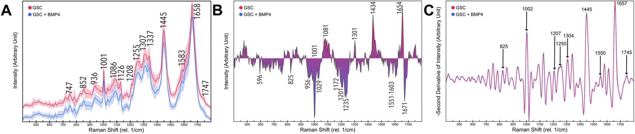

Fig. 3 (a) Mean Raman spectra of Glioblastoma stem cells (red) and differentiated Glioblastoma cells (blue) and their standard deviation in 1146 measurements. (b) The difference traces calculated by subtraction of Raman spectra of distinguished Glioblastoma cells (negative) from Glioblastoma stem cells (positive) (c) Negative Savitzky–Golay filtered second derivative of Glioblastoma stem cells (red) and differentiated Glioblastoma cells (blue).

2 Description of cell line heterogeneity

To account for the heterogeneity of the tumor and correspondingly the molecular genetic profile of the cell lines, we further outline cell line differences. The mean spectra of each cell line are shown in Fig. 4a, peak contributions are elaborated in a negative second derivative calculated by Savitzky–Golay filter in Fig. 4b. The difference traces of GCS signals separated from DGC intensities are shown in Fig. 4c. The generation of these spectra is grounded on the allocation of the measurement points as illustrated in Table 1 before.

Fig. 4 (a) Mean values and standard deviation of Raman spectroscopic measurements of HST-GBM1, NCH644, JHH620, BTSC-407, and BTSC233 including background (arbitrary units). (b) Negative Savitzky–Golay filtered the second derivative of each cell line. (c) The difference traces calculated by subtraction of Raman spectra of distinguished Glioblastoma cells (negative) from Glioblastoma stem cells (positive) within each cell line.

3 Stratification of biological clusters associated with cellular organelles

To allocate individual measurements inside the cell, K-means clustering (k = 4) assigns all single-point measurements and shows peak contribution in Fig. 5a and b of each cluster. The distribution of measurements among the clusters is composed as listed hereafter: 600 counts in cluster 1, 67 counts in cluster 2, 406 counts in cluster 3, and 73 counts in cluster 4. Each cluster could be associated with specific fingerprints of putative cell compartments. To verify clusters are preserving most measurement information, the corresponding principal component analysis (PCA) is depicted in Fig. 5c with color-coding of clusters illustrating the first three components that explain 60% of the total variation.

Fig. 5 (a) Negative Savitzky–Golay filtered the second derivative of 4 cell clusters by k-Means. Labeled areas elucidate important differences among the clusters with outstanding amounts of nucleic acids in cluster 2 and lipid contents in cluster 4. (b) Mean spectra of clusters 1–4 and their standard deviation. (c) Principal component analysis of all measurements imaging principal components 1–3 with a total variation of 60%. Colorization uncovers the main distribution of variation along these clusters.

Distribution of peaks in cluster 1 correlate to the cell nucleus: the range of 600–800 cm⁻¹ can be associated with the ring stretching vibrations of DNA/RNA.³⁹ The wave numbers 783 cm⁻¹ and 825 cm⁻¹ are typical peaks derived from nucleic acids, their pyrimidine rings, and asymmetrical PO2 double bonds.⁴⁰ Peak 1087 cm⁻¹ is assigned to symmetric stretching of phosphate.⁴⁰ 1583 cm⁻¹ represents the C=C stretching of purine.³⁹ The findings indicate that the spectra are derived from an area with a high DNA/RNA concentration, as expected in the cell nucleus.

Cluster 2 is characterized by the presence of intense Raman peaks at the following positions: 747, 1127, 1312, and 1584 cm⁻¹. These bands can be attributed to cytochrome c,⁴¹ suggesting that cluster 2 can be identified as rich in mitochondria.

Clusters 3 seems related to cluster 1, while cluster 3 has higher fatty acid and lipid peaks which can be assigned to C–N bonds in membrane phospholipids.⁴² Presumably, cluster 3 contains a higher membrane content. In addition to portions of the cell membrane, the distribution pattern of cluster 3 shows water content and correlation with proteins of cytoplasmic origin.⁴³

Cluster 4 has increased values at 863, 1071, 1263, 1301, 1439, 1656, and 1745 cm⁻¹. Peaks in the area of 1000–1200 cm⁻¹ and bands around 1301 cm⁻¹ and 1439 cm⁻¹ are known to originate from fatty acids.⁴³ Bands at 1263, 1301, 1439, and 1656 cm⁻¹ are distinctive of diverse contents attributed to lipids.³⁹ The peak at the wavenumber 1745 cm⁻¹ can be attributed to C=O stretching found in the ester group of lipids and phospholipids.⁴⁴ It is likely that cluster 4 is measured within a fatty cell component with high lipid concentrations like lipid droplets or lipid vesicles. We further guided our findings through reference cell imaging as shown in Fig. 6. As reference, a sketch of cell compartments is shown in Fig. 6a with assignment of cluster 1 to the nucleus, cluster 2 to mitochondria, cluster 3 to the cytoplasm with different densities of biological mass and membrane involvement and cluster 4 to a lipid-rich cell organelle, like lipid vesicles or lipid droplets. The color-coded integral of the Raman intensity (400–3700 cm⁻¹) with a Raman spectroscopic resolution of 500 nm across a 20 μm^2 area illustrates measurements of a BTSC-233 GSC cell (Fig. 6b). K-means clustering (k = 5 including background) illustrates comparable subgroups to the clustering of single-point measurements (Fig. 6c). Fig. 6d and e shows a treated HSR-GBM1 DGC counterpart and its Raman intensity (400–3700 cm⁻¹) and comparable clustering by k-means. The mean spectra of each cluster in treated and untreated conditions are shown in Fig. 6f (untreated) and Fig. 6g (treated) serving as references for our previous endeavoured cell organelle classification.

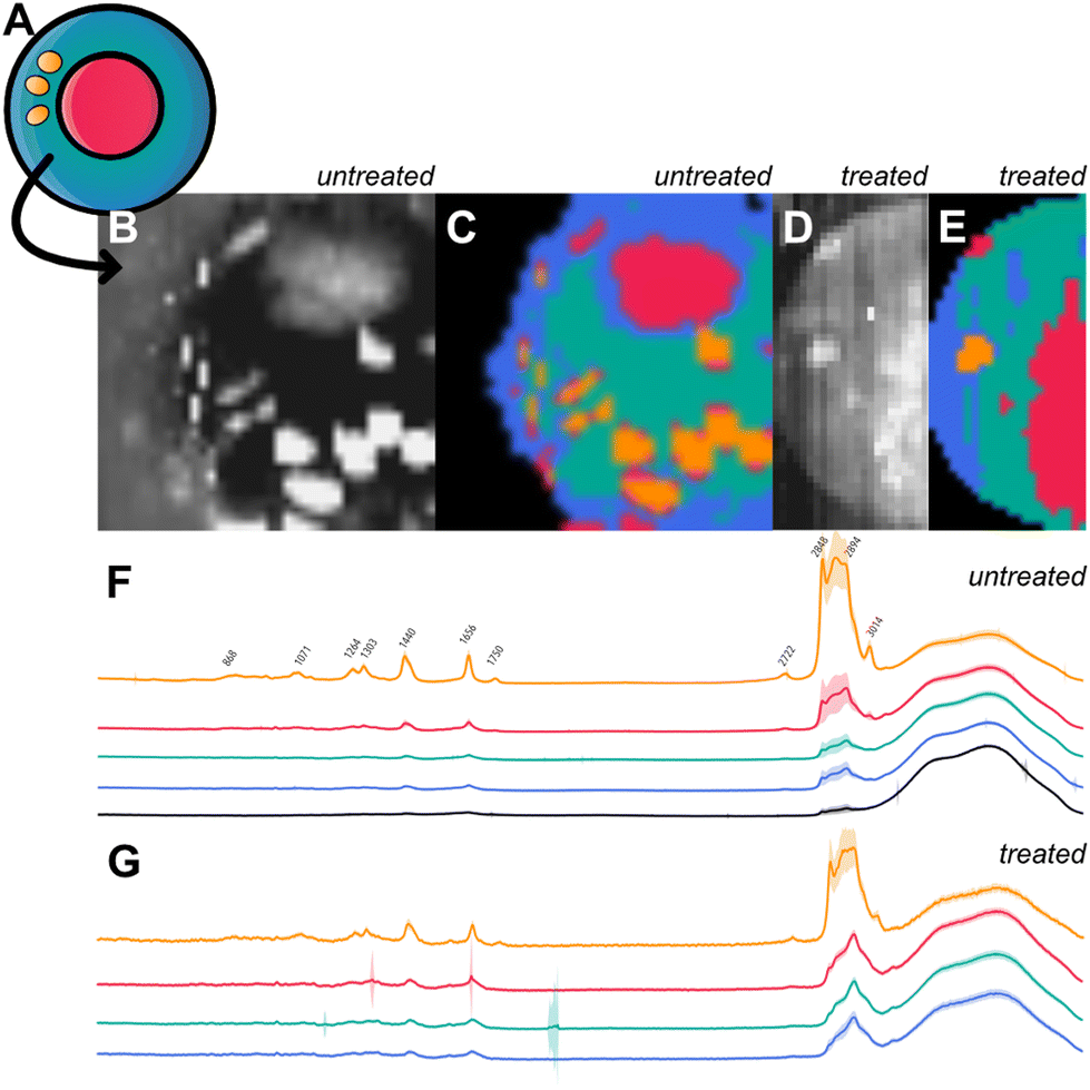Fig. 6 (a) Cell sketch highlights the estimated correlation between cell compartment clustering and spectroscopic content. It illustrates the attribution of clusters 1 being nucleus, cluster 2 assigned as mitochondria-rich, cluster 3 containing cytoplasm plus membrane content and cluster 4 as lipid droplets. (b) Raman brightness-coded hyper-spectral image of a single BTSC-233 Glioblastoma stem cell (resolution 500 nm across 20 μm² area, 400–3700 cm⁻¹) illustrates cell organelles. (c) K-Means clustering (k = 5 including background) showscluster distribution as described for the single-point measurements. (d) Raman brightness-coded hyper-spectral image of a single HSR-GBM1 BMP4 treated cell (resolution 250 nm across 15 μm² area, 400–3700 cm⁻¹) (e) K-means clustering of HSR-GBM1 cell (f) mean spectra and standard deviation of Raman GSC BTSC-233 image clustering (arbitrary units, 400–3700 cm⁻¹) (g) mean spectra and standard deviation of Raman DGC HSR-GBM1 image clustering (arbitrary units, 400–3700 cm⁻¹).

4 Description of GSC characteristics in identified cellular organelles

Spectral differences between both treatment conditions of each cluster may offer potential insights into chemical and metabolic changes within the respective compartments and thus, phenotypic differences. Fig. 7 shows the difference traces between clusters. As our study focuses on these differences, a list of promising peaks is listed hereafter:

Primary areas of GSCs in cluster 1 can be described in the areas with the most prominent peaks at 783, 1093, 1307, 1334, 1375, 1485, 1490 and 1576 cm⁻¹. DGCs are characterized most distinguishably by dominant signals at 953, 1001, 1030 cm⁻¹ and 1670 cm⁻¹.

Fig. 7 The difference traces calculated by subtraction of Raman spectra of distinguished Glioblastoma cells (negative) from Glioblastoma stem cells (positive) in k-Means (k = 4) clustered cell compartments.

The main differences in cluster 2 predominant in GSCs are around 936, 1110, 1333, 1382 and 1653 cm⁻¹, DGCs show highest peaks at 693, 747, 1174, 1311 and 1592 cm⁻¹.

In cluster 3, the main areas of the GSC fraction are 1050 and 1435 cm⁻¹. The main areas of the DGC fraction are leading at 786, 1256, 1371, 1482 and 1577 cm⁻¹.

Cluster 4 contains GSC leading areas around 1261, 1438 and especially 1657 cm⁻¹ has a high intensity. DGC dominating areas can be observed at 1001, 1128, 1337, 1579 and 1680 cm⁻¹.

5 Machine learning classification identifies the most characteristic peaks for discriminating tumor stem cells, which can be used as stand-alone markers for stratification

To derive a prediction from the results in an application-driven manner, automatic preprocessing steps, LDA, PCA, and machine learning algorithms were applied, and parameters of all algorithms were optimized to achieve highest accuracy. LDA achieves a discrimination accuracy of 54%. Absolute scaling values of SciKits LDA show each peaks relevance for stem cell feature discrimination, highlighting the highest peaks at 1685, 1018, 963, 1591, 1622, 1334 and 1655 cm⁻¹ to have a potential effect for discrimination as seen in Fig. 8a.

Fig. 8 (a) Scikit-learnscalings from Linear Discriminant Analysis highlighting the origin of its classification. (b) Differentiated Glioblastoma cells (treated by BMP4) and Glioblastoma stem cells (untreated cell culture) and their subdivision by Linear Discriminant Analysis (LD1). The training dataset (red) is preferably separated compared to the testing dataset (blue).

Machine learning algorithms perform superior according to Table 2. An overall accuracy of 60.3% can be achieved by k Nearest-Neighbors algorithm (Table 2a). Best predictions within each cell component are 57.3% in cluster 1/nucleus by k Nearest-Neighbors, 72.7% in cluster 2/mitochondria by AdaBoost and Tree Classification, 63.1% in cluster 3/cytoplasm by Naive Bayes and 91.7% in cluster 4/lipid droplets by Stochastic Gradient Descending (Table 2b).

Table 2 Glioblastoma stem cell (GSC) classification performance of ten state-of-the-art machine learning algorithms measured by a random 20% test dataset

Algorithms	Accuracy (%)^a	Precision (%)	Recall (%)	Accuracy of cluster 1 (%)^b	Accuracy of cluster 2 (%)	Accuracy of cluster 3 (%)	Accuracy of cluster 4 (%)	Accuracy of HSR-GBM1 (%)^c	Accuracy of JHH520 (%)	Accuracy of NCH644 (%)	Accuracy of BTSC-407 (%)	Accuracy of BTSC-233 (%)
a Accuracy (main target), precision, and recall of GSC prediction. b GSC classification, accuracy of each cluster/cell compartment. c GSC classification, accuracy of each cell line.
Artificial Neural Network	54.9	55.7	54.9	51	63.6	58.5	66.7	62.2	58.3	51.2	59.4	65.8
Support Vector Machine	51.6	50.3	51.6	55.2	63.6	56.9	66.7	56.8	52.8	58.1	62.5	57.9
Stochastic Gradient Descending	47.8	51.4	47.8	47.9	63.6	53.8	91.7	62.2	55.6	55.8	59.4	52.6
k Nearest Neighbour	60.3	62.9	60.3	57.3	63.6	58.5	33.3	59.5	63.9	58.1	71.9	52.6
Logistic Regression	47.8	51.2	47.8	45.8	54.5	52.3	83.3	59.5	55.6	55.8	56.2	52.6
Gradient Boosting	50.5	52.9	50.5	47.9	18.2	60	50	54.1	36.1	58.1	62.5	63.2
AdaBoost	56	59.1	56	49	72.7	56.9	41.7	48.6	41.7	48.8	65.6	60.5
Random Forest	53.3	56.8	53.3	50	54.5	52.3	58.3	45.9	52.8	67.4	71.9	55.3
Tree	54.9	57.2	54.9	50	72.7	41.5	58.3	59.5	63.9	53.5	34.4	52.6
Naive Bayes	48.4	49.7	48.4	52.6	63.6	63.1	75	73	55.6	62.8	62.5	42.1

---

In cell lines, the best predictions are 73% in HSR-GBM1 by Naive Bayes, 63.9% in JHH520 by k Nearest-Neighbors, 67.4% in NCH644 by Random Forrest, 71.9% in BTSC-407 by Random Forrest and 63.2% in BTSC-233 by Gradient Boosting (Table 2c).

As we are aiming to use the algorithms in surgical practice on larger areas of tissue, the time of acquisition of data that might be defining of GSC residence must be as short as possible. Time can be saved significantly by narrowing the focus of data acquisition to a few selected peaks instead of the entire spectrum acquisition. Considering the described results on putative biological stratification and scaling of the algorithms, we performed a feature selection of distinct peaks from our previous analysis and biological review for the most promising cell compartments. Selecting the top five LDA scaling values, as seen in Fig. 7a, achieves 65.3% accuracy by ANN (Precision 0.681, Recall 0.653) in cluster 2. Narrowing the number of peaks in lipid organelles while still using PCA achieves likewise results of 91.7% by ANN. Selection of up to 10 out of all leading lipid-rich peaks results in a maximum accuracy of 69.4% by SVM (Precision 0.708, Recall 0.694), selection of single peaks achieves an accuracy of up to 63% for 1001 cm⁻¹. Interestingly 1001 cm⁻¹ (associated with tryptophan) scores 80% (Precision 0.81; Recall 0.80) by Tree classification in cluster 2 (cytochrome c-rich compartment).

D Discussion

Over the last two decades, establishing methods for specific identification of tumor stem cells based on putative biomarkers has been the center of various research projects worldwide. Yet, none of the discoveries has entered clinical routine, mostly due to inefficient repeatability of preclinical results in human settings, and conflicting evidence on the utility of the proposed biomarker to unequivocally stratify stem cells from non-cancer stem cells.^20,45–47 Our project associates to this long endeavour but with new innovation that makes us believe our approach has the utility to enter clinical application in the future, due to it's (a) computational based fundament minimizing human operator introduced bios/errors in data interpretation meanwhile elevating the recognition of hitherto never described biomarker discovery and (b) – building up on previous successes of others proving the potential of the rapidity of result generation using Raman spectroscopy^{13,14,21,48,49} – the theoretical realistic implementation in fast pace intraoperative setting.

We hypothesize these statements based on the fact that very recently, machine learning- and deep learning-supported Raman spectroscopy diagnostics has innovated a wide range of sectors in biology and medicine, such as food quality control^50,51 or pathogen analytics⁵² incl. the establishment of a rapid SARS-CoV2 diagnostics that circumvents the long waiting times for the results when using amplification-based PCR tests, meanwhile maintaining high specificity and sensitivity of the test.⁵³ Regarding cancer, machine learning-assisted Raman spectroscopy diagnostics was recently shown to allow the stratification of tumors that are resistant to immune therapy,⁵⁴ raising hopes to improve the economic effectivity of these revolutionary but certainly very cost-intense cancer therapies. Moreover, machine learning Raman spectroscopy can also classify neural differentiation stages of human induced pluripotent stem cells⁵⁵ or neural stem cells.²⁵

Based on our experimental setup, we focus our discussion on the clustered cell organelles as well as a few novel selected peaks that we found of most relevance and interest due to the amplitude of differences between GSC and DSC and the previous work of others that associate those signals with biological processes.

In general, GSCs have prevailing areas indicating mainly a greater lipid concentration and different protein structure of amide I and III: 1304 cm⁻¹ is assigned to the CH2 deformation of lipids, 1435–1439 cm⁻¹ is attributed to lipids CH2 scissoring, CH2 bending mode, and CH2 deformation. 1447 cm⁻¹ is a common peak of lipids, fatty acids, phospholipids, and methylene groupings such as CH2 and CH₃. 1650–1658 cm⁻¹ is typical for the v(C=C) stretch of lipids and fatty acids. It is also assigned to a-helix structure and amide I. 1550 cm⁻¹ can be further described by tryptophan and NADH.⁴² Significantly higher peaks of DGCs at 407 and 411 cm⁻¹ can be attributed to saccharide.^55,56

Savitzky–Golay filtered negative second-derivative confirms noticeable differences by finding an increase of 1207 cm⁻¹ and 1250 cm⁻¹ in DGCs, which complies with the ring breathing mode of hydroxyproline, tryptophan, phenylalanine, adenosine and tyrosine, as also guanine, cytosine and amide III. 1745 cm⁻¹ is increased in GSCs and assigned to the C=O stretch of lipid esters, triglycerides, and phospholipids.⁴²

Regarding machine learning classification, main scaling values of LDA can be correlated to protein (963, 1591 cm⁻¹), especially amide 1 (1655, 1685 cm⁻¹), ribose (1018 cm⁻¹), nucleic acids (1655 cm⁻¹) and lipids (1655 cm⁻¹), which follows our findings. Besides confocal measurements, our machine learning algorithms faced the challenge of heterogenic cell lines. Considering this limitation, a general prediction of 60.3% across all organelles is the result of overfitting. This is underlined by the inability of the most promising algorithms like SVM and ANN, which are particularly vulnerable to overfitting despite parameter optimization.

To accentuate the impact and challenge towards the biological limitation in GBM, we would like to discuss our cell line response: regarding tumor heterogeneity, we found that the described cell line transcriptomes of our previous studies and the spectral profiles share affinities, as well as a strong correlation with the cell line response to BMP4 as published earlier by our laboratory.³⁴ Exemplary, the more responsive 407p can be more accurately classified with 71.9% compared to JHH520 with 63.9%.

As in compliance with our measurement setup, we overcome limitation of confocal measurements by automatic cell organelle classification. This further allows a detailed description of differences in GSCs and DGCs in each compartment: it has been described that cluster 1 has its origin in the nucleus while cluster 3 showed similarities and was described to have a cytoplasmic origin due to the water distribution and absence of characteristic peaks, as also partly membrane origin. GSCs seem to have higher content of nucleic acids in cluster 1, because of higher areas at 784, 1483–1491 and 1575–1579 cm⁻¹. On the other hand, DGCs have higher nucleic acid content in cluster 3 in similar areas at 784, 1371, 1487, 1575–1583 cm⁻¹. GSCs also have higher amounts of lipids in cluster 1 around 1375 cm⁻¹, and CH2 groups around 1431–1447 cm⁻¹ in cluster 3. DGCs are leading in phenylalanine in cluster 1 at 1001–1005 and in cluster 3 at 1583 cm⁻¹. They also show higher amide I bands at 1665–1573 cm⁻¹ in cluster 1. Thus, we confirmed the former findings by identifying higher lipid quantity in GSCs and showed larger amide I bands in DGCs cytoplasm.³⁹ Additionally, the shift of nucleic acids from cluster 1 to cluster 3 during differentiation could be a potential conduct of GSCs. The propagation of nucleic acids in cluster 3, an estimated membrane content like rough endoplasmic reticulum, could be debated as increased transcription because of higher RNA content near the ribosomes. Because nucleic acids were identified as a main target for stem cell identification in previous findings, further research is needed to reveal deeper insights into the changes in nucleic acids in stem cells.⁵⁷ We find main intensities in GSCs at 1439 cm⁻¹ and 1650–1662 cm⁻¹ in the liposomal cluster 4. These areas are described as lipids, CH2, CH₃, v(C=C) cis of phospholipids, triglycerides, cholesterol band, ceramide backbone, and C=C groups of unsaturated fatty acids. The quotient of the peak intensities at 1656 cm⁻¹/1444 cm⁻¹ is often used as an approximation of the unsaturation degree in fatty acids. In this cluster, GSCs have a 3.31% higher amount of unsaturated lipids.^43,58

After clustering, we extracted great results of 91.7% in lipid organelles, which we discussed as lipid droplets. This matches the reports published about lipid droplets in stem cells being differently configured than their differentiated progeny.^45,59–61 One inference for the obtained favourable performance against the limited quantity of measurements may be the very intense Raman signal of the lipid bands, as well as the biological valence of these organelles. Regarding clinical usage, an intracellular measurement inside a lipid organelle would lead to a confident hit above 90%. Building on this potential, we strongly recommend that this structure be verified and subjected to more rigorous analysis in follow-up work. Expanding on these foundations, additional follow-up work could elaborate on our features to improve classification success. This could be achieved through examining feature importances from random forest and XgBoost, the coefficient values from linear SVC or employing penalised logistic regression (such as LASSO or elastic net penalty) to reduce the number of necessary features for modelling purposes.

Importantly, our data also suggests the realization of GSC detection of selected stand-alone markers as described in results, which could give a huge opportunity for intraoperative application. We speculate that the selection of 4–5 peaks out of over 1400 peaks in general or with focus on enhanced cytochrome signals and lipid bands will give a significant reduction of time for recording compared to total spectra recording allowing the rapid scanning of various cm of length, feasible to be conducted in an intraoperative setting.

From a surgical standpoint of view, our study has limitations, when it comes to speculating on the clinical potential of our results per se. Firstly, although our applied disease model systems have recently been shown to present a solid basis for repeatable research and recapitulate core molecular parameters of patient tumors,³³ facts which we find a fundamental basis to argue any potential translational relevance of our in vitro data, the entire data was generated in pure experimental conditions. Confirmatory studies on fresh tumor material, whether upon short-term in vitro processing or direct tumor resection specimens, are needed to verify our hypothesis. Since we envision to use hand hold Raman devices,⁶² we do not think ex vivo applications such as simulated with imaging on xenograft in vivo models of cancers are relevant to benchmark our assay for its applicability. Secondly, the Raman microscope applied is a high-end instrument purchased primarily to perform highly sensitive spatially resolved analyses in materials science. It requires verification if our Raman signals can be detected equally with a putatively transferable system in the operation room.

E. Conclusions

We successfully evaluated the preclinical usability of confocal Raman spectroscopic and machine learning-guided approach to classifying tumor stem cells from non-tumor stem cells in vitro. Tailoring machine learning-based identification of differences of tumor stem cells Raman spectra in clusters and to a few selected peaks, we introduce new standalone diagnostic opportunities. Our results suggest these results are based on biological alterations of lipids and proteins in GCSs and mainly in lipid-rich organelles. However, confirmatory studies on fresh tumor resection specimens or in-man applications using an instrumental setup that can be implemented in operation room processes are needed to make conclusive statements regarding our data's clinical relevance. As a starting point, our work highlights machine learning and deep learning network computation combined with Raman spectroscopy having the potential to innovate surgical oncology and guide neurosurgical decision-making towards better treatment options and patient outcome.

Author contributions

Conceptualization, L.W., M.H., B.F. and U.K.; methodology, L.W. and B.F.; software, L.W. and B.F.; validation, L.W., D.R., I.F., V.N., R.C., M.H., B.F., J.D. and U.K.; formal analysis, L.W. and I.F.; investigation, L.W., I.F., V.N., R.G., R.C., M.H., B.F. and U.K.; resources, L.W., B.F. and U.K.; data curation, L.W. and B.F.; writing—original draft preparation, L.W.; writing—review and editing, D.R., I.F., V.N., R.G., R.C., M.H., B.F., J.D. and U.K.; visualization, L.W.; supervision, M.H., B.F., J.D. and U.K.; project administration, L.W., B.F. and U.K.; funding acquisition, M.H., B.F. and U.K. All authors have read and agreed to the published version of the manuscript.

Conflicts of interest

B.F. is the managing director of FISCHER GmbH. The company performed the Raman measurements. The other authors declare no competing interests.

Acknowledgements

We thank Michael Hewera and Ann-Christin Nickel for their laboratory support.

References

1. K. D. Miller, L. Nogueira, A. B. Mariotto, J. H. Rowland, K. R. Yabroff, C. M. Alfano, A. Jemal, J. L. Kramer and R. L. Siegel, CA-Cancer J. Clin., 2019, 69, 363–385.
2. S. K. Perera, S. Jacob, B. E. Wilson, J. Ferlay, F. Bray, R. Sullivan and M. Barton, Lancet Oncol., 2021, 22, 182–189.
3. R. L. Siegel, K. D. Miller, H. E. Fuchs and A. Jemal, CA-Cancer J. Clin., 2021, 71, 7–33.
4. G. Tabatabai and M. Weller, Cell Tissue Res., 2011, 343, 459–465.
5. S. J. Sundar, J. K. Hsieh, S. Manjila, J. D. Lathia and A. Sloan, Neurosurg. focus, 2014, 37(6), E6.
6. S. Bao, Q. Wu, R. E. McLendon, Y. Hao, Q. Shi, A. B. Hjelmeland, M. W. Dewhirst, D. D. Bigner and J. N. Rich, Nature, 2006, 444, 756–760.
7. A. L. V. Alves, I. N. F. Gomes, A. C. Carloni, M. N. Rosa, L. S. Da Silva, A. F. Evangelista, R. M. Reis and V. A. O. Silva, Stem Cell Res. Ther., 2021, 12(1), 206.
8. N. Takebe, L. Miele, P. J. Harris, W. Jeong, H. Bando, M. Kahn, S. X. Yang and S. P. Ivy, Nat. Rev. Clin. Oncol., 2015, 12, 445–464.
9. K. Biserova, A. Jakovlevs, R. Uljanovs and I. Strumfa, Cells, 2021, 10, 621.
10. R. Stupp, W. P. Mason, M. J. Van Den Bent, M. Weller, B. Fisher, M. J. Taphoorn, K. Belanger, A. A. Brandes, C. Marosi and U. Bogdahn, N. Engl. J. Med., 2005, 352, 987–996.
11. U. Kahlert, G. Nikkhah and J. Maciaczyk, Cancer Lett., 2013, 331, 131–138.
12. J. D. Lathia, S. C. Mack, E. E. Mulkearns-Hubert, C. L. Valentim and J. N. Rich, Genes Dev., 2015, 29, 1203–1217.
13. B. Broadbent, J. Tseng, R. Kast, T. Noh, M. Brusatori, S. N. Kalkanis and G. W. Auner, J. Neuro-Oncol., 2016, 130, 1–9.
14. T. Hollon, S. Lewis, C. W. Freudiger, X. S. Xie and D. A. Orringer, Neurosurg. focus, 2016, 40(3), E9.
15. F.-K. Lu, D. Calligaris, O. I. Olubiyi, I. Norton, W. Yang, S. Santagata, X. S. Xie, A. J. Golby and N. Y. R. Agar, Cancer Res., 2016, 76, 3451–3462.
16. H. J. Butler, L. Ashton, B. Bird, G. Cinque, K. Curtis, J. Dorney, K. Esmonde-White, N. J. Fullwood, B. Gardner, P. L. Martin-Hirsch, M. J. Walsh, M. R. McAinsh, N. Stone and F. L. Martin, Nat. Protoc., 2016, 11, 664–687.
17. C. Aksoy and F. Severcan, Spectroscopy, 2012, 27, 167–184.
18. H. Karabeber, R. Huang, P. Iacono, J. M. Samii, K. Pitter, E. C. Holland and M. F. Kircher, ACS Nano, 2014, 8, 9755–9766.
19. J. Desroches, M. Jermyn, M. Pinto, F. Picot, M.-A. Tremblay, S. Obaid, E. Marple, K. Urmey, D. Trudel and G. Soulez, Sci. Rep., 2018, 8, 1–10.
20. S. Schipmann, M. Schwake, E. Suero Molina and W. Stummer, J. Neurol. Surg. Part A, 2019, 80(6), 475–487.
21. D. DePaoli, É. Lemoine, K. Ember, M. Parent, M. Prud'homme, L. Cantin, K. Petrecca, F. Leblond and D. C. Côté, J. Biomed. Opt., 2020, 25, 050901.
22. D. Reinecke, N. Von Spreckelsen, C. Mawrin, A. Ion-Margineanu, G. Fürtjes, S. T. Jünger, F. Khalid, C. W. Freudiger, M. Timmer, M. I. Ruge, R. Goldbrunner and V. Neuschmelting, Acta Neuropathol. Commun., 2022, 10, 109.
23. R. Gautam, S. Vanga, F. Ariese and S. Umapathy, EPJ Tech. Instrum., 2015, 2, 1–38.
24. L. J. Livermore, M. Isabelle, I. M. Bell, C. Scott, J. Walsby-Tickle, J. Gannon, P. Plaha, C. Vallance and O. Ansorge, Neuro-Oncol. Adv., 2019, 1, vdz008.
25. J. Geng, W. Zhang, C. Chen, H. Zhang, A. Zhou and Y. Huang, Anal. Chem., 2021, 93, 10453–10461.
26. S. N. Kalkanis, R. E. Kast, M. L. Rosenblum, T. Mikkelsen, S. M. Yurgelevic, K. M. Nelson, A. Raghunathan, L. M. Poisson and G. W. Auner, J. Neuro-Oncol., 2014, 116, 477–485.
27. S. Kumar, A. Visvanathan, A. Arivazhagan, V. Santhosh, K. Somasundaram and S. Umapathy, Anal. Chem., 2018, 90, 12067–12074.
28. D. Garnier, O. Renoult, M.-C. Alves-Guerra, F. Paris and C. Pecqueur, Front. Oncol., 2019, 9, 118.
29. Y. Zhou, C.-H. Liu, B. Wu, X. Yu, G. Cheng, K. Zhu, K. Wang, C. Zhang, M. Zhao and R. Zong, J. Biomed. Opt., 2019, 24, 095001.
30. N. Feuerer, D. A. Carvajal Berrio, F. Billing, S. Segan, M. Weiss, U. Rothbauer, J. Marzi and K. Schenke-Layland, Biomedicines, 2022, 10, 989.
31. V. Revin, L. Balykova, S. Pinyaev, I. Syusin, O. Radaeva, N. Revina, Y. Kostina, E. Kozlov, V. Inchina, I. Nikitin, A. Salikov and I. Fedorov, Biomedicines, 2022, 10, 553.
32. I. P. Santos, E. M. Barroso, T. C. Bakker Schut, P. J. Caspers, C. G. F. Van Lanschot, D.-H. Choi, M. F. Van Der Kamp, R. W. H. Smits, R. Van Doorn, R. M. Verdijk, V. Noordhoek Hegt, J. H. Von Der Thüsen, C. H. M. Van Deurzen, L. B. Koppert, G. J. L. H. Van Leenders, P. C. Ewing-Graham, H. C. Van Doorn, C. M. F. Dirven, M. B. Busstra, J. Hardillo, A. Sewnaik, I. Ten Hove, H. Mast, D. A. Monserez, C. Meeuwis, T. Nijsten, E. B. Wolvius, R. J. Baatenburg De Jong, G. J. Puppels and S. Koljenović, Analyst, 2017, 142, 3025–3047.
33. A. Nickel, D. Picard, N. Qin, M. Wolter, K. Kaulich, M. Hewera, D. Pauck, V. Marquardt, G. Torga and S. Muhammad, Biomed. Pharmacother., 2021, 144, 112278.
34. K. Koch, R. Hartmann, A. K. Suwala, D. H. Rios, M. A. Kamp, M. Sabel, H.-J. Steiger, D. Willbold, A. Sharma, U. D. Kahlert and J. Maciaczyk, Cancers, 2021, 13, 6001.
35. L. T. Kerr, H. J. Byrne and B. M. Hennelly, Anal. Methods, 2015, 7, 5041–5052.
36. F. Pedregosa, G. Varoquaux, A. Gramfort, V. Michel, B. Thirion, O. Grisel, M. Blondel, P. Prettenhofer, R. Weiss and V. Dubourg, J. Mach. Lear. Res., 2011, 12, 2825–2830.
37. J. Demšar, T. Curk, A. Erjavec, Č. Gorup, T. Hočevar, M. Milutinovič, M. Možina, M. Polajnar, M. Toplak and A. Starič, J. Mach. Lear. Res., 2013, 14, 2349–2353.
38. S. Wartewig, IR and Raman spectroscopy: fundamental processing, John Wiley & Sons, 2006.
39. J. De Gelder, K. De Gussem, P. Vandenabeele and L. Moens, J. Raman Spectrosc., 2007, 38, 1133–1147.
40. Y. Chen, J. Dai, X. Zhou, Y. Liu, W. Zhang and G. Peng, PLoS One, 2014, 9, e93906.
41. M. Okada, N. I. Smith, A. F. Palonpon, H. Endo, S. Kawata, M. Sodeoka and K. Fujita, Proc. Natl. Acad. Sci. U. S. A., 2012, 109, 28–32.
42. Z. Movasaghi, S. Rehman and I. U. Rehman, Appl. Spectrosc. Rev., 2007, 42, 493–541.
43. C. Krafft, I. Schie, T. Meyer, M. Schmitt and J. Popp, Chem. Soc. Rev., 2016, 45, 1819–1849.
44. C. Matthäus, T. Chernenko, C. Stiebing, L. Quintero, M. Miljković, L. Milane, A. Kale, M. Amiji, S. Lorkowski, V. Torchilin, J. Popp and M. Diem, Confocal Raman Microscopy, Springer International Publishing, 2018, pp. 273–305,  DOI:10.1007/978-3-319-75380-5_13.
45. I. Notingher, I. Bisson, J. M. Polak and L. L. Hench, Vib. Spectrosc., 2004, 35, 199–203.
46. A. Downes, R. Mouras, P. Bagnaninchi and A. Elfick, J. Raman Spectrosc., 2011, 42, 1864–1870.
47. O. Uckermann, R. Galli, M. Anger, C. Herold-Mende, E. Koch, G. Schackert, G. Steiner and M. Kirsch, Int. J. Radiat. Biol., 2014, 90, 710–717.
48. R. Galli, O. Uckermann, T. Sehm, E. Leipnitz, C. Hartmann, F. Sahm, E. Koch, G. Schackert, G. Steiner and M. Kirsch, J. Biophotonics, 2019, 12, e201800465.
49. T. C. Hollon, B. Pandian, A. R. Adapa, E. Urias, A. V. Save, S. S. S. Khalsa, D. G. Eichberg, R. S. D'Amico, Z. U. Farooq, S. Lewis, P. D. Petridis, T. Marie, A. H. Shah, H. J. L. Garton, C. O. Maher, J. A. Heth, E. L. McKean, S. E. Sullivan, S. L. Hervey-Jumper, P. G. Patil, B. G. Thompson, O. Sagher, G. M. McKhann, R. J. Komotar, M. E. Ivan, M. Snuderl, M. L. Otten, T. D. Johnson, M. B. Sisti, J. N. Bruce, K. M. Muraszko, J. Trautman, C. W. Freudiger, P. Canoll, H. Lee, S. Camelo-Piragua and D. A. Orringer, Nat. Med., 2020, 26, 52–58.
50. S. Yan, S. Wang, J. Qiu, M. Li, D. Li, D. Xu, D. Li and Q. Liu, Talanta, 2021, 226, 122195.
51. S. Hu, H. Li, C. Chen, C. Chen, D. Zhao, B. Dong, X. Lv, K. Zhang and Y. Xie, Sci. Rep., 2022, 12, 3456.
52. S. Yu, X. Li, W. Lu, H. Li, Y. V. Fu and F. Liu, Anal. Chem., 2021, 93, 11089–11098.
53. D. Paria, K. S. Kwok, P. Raj, P. Zheng, D. H. Gracias and I. Barman, Nano Lett., 2022, 22(9), 3620–3627.
54. S. K. Paidi, J. Rodriguez Troncoso, P. Raj, P. Monterroso Diaz, J. D. Ivers, D. E. Lee, N. L. Avaritt, A. J. Gies, C. M. Quick, S. D. Byrum, A. J. Tackett, N. Rajaram and I. Barman, Cancer Res., 2021, 81, 5745–5755.
55. C.-C. Hsu, J. Xu, B. Brinkhof, H. Wang, Z. Cui, W. E. Huang and H. Ye, Proc. Natl. Acad. Sci. U. S. A., 2020, 117, 18412–18423.
56. I. R. M. Ramos, A. Malkin and F. M. Lyng, BioMed Res. Int., 2015, 2015, 561242.
57. A. Ghita, F. C. Pascut, M. Mather, V. Sottile and I. Notingher, Anal. Chem., 2012, 84, 3155–3162.
58. A. Kaczor, K. M. Marzec, K. Majzner, K. Kochan, M. Z. Pacia and M. Baranska, in Confocal Raman Microscopy, Springer, 2018, pp. 307–346.
59. F. Geng, X. Cheng, X. Wu, J. Y. Yoo, C. Cheng, J. Y. Guo, X. Mo, P. Ru, B. Hurwitz, S.-H. Kim, J. Otero, V. Puduvalli, E. Lefai, J. Ma, I. Nakano, C. Horbinski, B. Kaur, A. Chakravarti and D. Guo, Clin. Cancer Res., 2016, 22, 5337–5348.
60. L. Tirinato, F. Pagliari, T. Limongi, M. Marini, A. Falqui, J. Seco, P. Candeloro, C. Liberale and E. Di Fabrizio, Stem Cells Int., 2017, 2017, 1656053.
61. S. Shakya, A. D. Gromovsky, J. S. Hale, A. M. Knudsen, B. Prager, L. C. Wallace, L. O. F. Penalva, H. A. Brown, B. W. Kristensen, J. N. Rich, J. D. Lathia, J. M. Brown and C. G. Hubert, Acta Neuropathol. Commun., 2021, 9(1), 101.
62. M. Jermyn, K. Mok, J. Mercier, J. Desroches, J. Pichette, K. Saint-Arnaud, L. Bernstein, M.-C. Guiot, K. Petrecca and F. Leblond, Sci. Transl. Med., 2015, 7, 274ra219.

---

Footnote

† These authors contributed equally.

---