
 Open Access Article
 This Open Access Article is licensed under a Creative Commons Attribution-Non Commercial 3.0 Unported Licence
Weakly supervised anomaly detection coupled with Fourier transform infrared (FT-IR) spectroscopy for the identification of non-normal tissue†
Dougal
Ferguson
 *ab,
Alex
Henderson
ab,
Elizabeth F.
McInnes
c and
Peter
Gardner
ab
*ab,
Alex
Henderson
ab,
Elizabeth F.
McInnes
c and
Peter
Gardner
ab
aPhoton Science Institute, University of Manchester, Oxford Road, Manchester, M13 9PL, UK. E-mail: dougal.ferguson@manchester.ac.uk
bDepartment of Chemical Engineering, School of Engineering, University of Manchester, Oxford Road, Manchester, M13 9PL, UK
cSyngenta, International Research Centre, Jealott's Hill, Bracknell, RG42 6EY, UK
First published on 11th July 2023
Abstract
The detection and classification of histopathological abnormal tissue constituents using machine learning (ML) techniques generally requires example data for each tissue or cell type of interest. This creates problems for studies on tissue that will have few regions of interest, or for those looking to identify and classify diseases of rarity, resulting in inadequate sample sizes from which to build multivariate and ML models. Regarding the impact on vibrational spectroscopy, specifically infrared (IR) spectroscopy, low numbers of samples may result in ineffective modelling of the chemical composition of sample groups, resulting in detection and classification errors. Anomaly detection may be a solution to this problem, enabling users to effectively model tissue constituents considered to represent normal tissue to capture any abnormal tissue and identify instances of non-normal tissue, be it disease or spectral artefacts. This work illustrates how a novel approach using a weakly supervised anomaly detection algorithm paired with IR microscopy can detect non-normal tissue spectra. In addition to incidental interferents such as hair, dust, and tissue scratches, the algorithm can also detect regions of diseased tissue. The model is never introduced to instances of these groups, training solely on healthy control data using only the IR spectral fingerprint region. This approach is demonstrated using liver tissue data from an agrochemical exposure mouse study.
Introduction
In mid-infrared spectroscopy, mid-infrared radiation (IR) is directed at a sample to stimulate molecular vibrations that may be used to interrogate the sample in question. These vibrations are characteristic of the underlying molecule, with the superposition of multiple molecular vibration patterns creating unique spectral fingerprints for the different chemical compositions contained within complex biological samples. These in turn may be used for identification.1,2 In principle, when utilising vibrational spectroscopy for any form of classification in tissue, the superpositions of the sample groups are sufficiently different to be differentiable by learning algorithms. It has been shown that this approach can detect and classify a range of diseases across tissue.3–7 Regarding the classification of cancers within tissues, these methods have been extended to enable not only the differentiation between cancerous and non-cancerous tissues, but also the differentiation between different cancer types, their grade, and even the stage of the disease.8–13One issue with these techniques is that they require labelled instances of each tissue type that the user wishes to discriminate. This may be difficult to obtain for a variety of reasons: from difficulties surrounding the availability and access to expert pathologist annotations, issues regarding image registration between adjacent tissue sections, to the ready access to samples that possess instances of a rare disease. These classifier approaches may also be restricted to predicting data to one of the specific classes labelled by the researcher, requiring all analysed data to be grouped under one of these pre-specified labels. In hard classification techniques these analysed data are assigned a label following a direct classification boundary, such as majority voting irrespective of the vote count. Alternatively, soft classifiers estimate conditional class probabilities for assignment, taking into account the probability of all class assignments.14 In light of this labelling requirement, there is scope for the development of a technique that can operate weakly supervised with a single class, using a single class group of normal/control tissue sample data to identify abnormal tissue and data anomalies without the need of diseased tissue labelling or sampling.
In this paper a method for detecting and segmenting abnormal spectra across tissue will be presented. Specifically, interferents, diseased tissue, and mixed pixels are isolated. This is completed using only healthy control sample data to train an outlier detection classifier consisting of an ensemble Isolation Forest (herein IF) approach.15,16 This method has been developed to show how mechanisms can be utilised for discriminating spectra/regions in the sample in datasets for which a priori labels are not available. For the liver tissue sample data used in this paper, normal data is categorised as healthy liver hepatocytes, as the liver is largely made up of these cells. Anomalous data is therefore defined as that which is not considered healthy hepatocellular tissue data. Once identified, this anomalous data is confirmed through both visual matching of identified groups to whole slide images (WSI) of the tissue alongside retrospective analysis of returned spectral groups.
Isolation forest
The term isolation refers to the separation of one instance from the remainder of instances. Regarding the isolation of anomalies from a dataset, ordered random partitioning can be utilised. Many combinations of data partitions can separate a single datapoint from all others, isolating it. The recursive partitioning of these data can be represented in a form that resembles a tree, with the path length from the root to terminating node for these isolated data equating to a measure of anomaly. Generally, anomalous data can be isolated by random partitions at an earlier point than normal data. To illustrate, Fig. 1 shows a generated dataset of X and Y axis with multiple datapoints (β) made of two draws (X1, Y1 respectively) from a uniform distribution, with two outlier points (α) appended that do not belong to the same distribution. It is possible to isolate a single datapoint within this group using random partitioning in a recursive manner. When ordering these partitions the result resembles a decision tree structure. For a datapoint belonging to the normal set, it will take multiple partitions to isolate the datapoint as there are many of them existing in the same subspace, thus a larger pathlength in the IF. For outliers, it will take fewer partitions in theory to isolate, as they do not exist in the same subspace as the normal group, and therefore result in shorter pathlengths. Repeating the process multiple times allows for the creation of a forest (see Fig. 2) of these partition trees, with the average path length for the data observations’ isolation across this forest being a measure of normality to determine anomalies.17 This is the foundation of the IF technique.15,16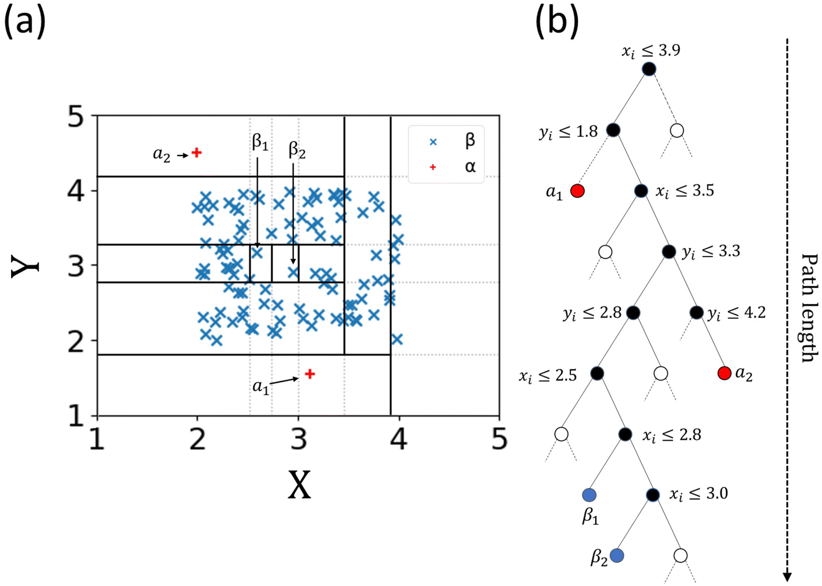 | ||
| Fig. 1 Outlier detection via an Isolation Forest algorithm approach. Random partitions of a dataset (solid black lines in (a), and black nodes in (b)) form decision nodes that isolate datapoints (solid blue nodes β1 and β2 and solid red nodes α1 and α2 respectively) after a certain number of splits. The number of splits represents the pathlength. Blank nodes represent further splits that continue but are not plotted for clarity. Generally, outliers will have a shorter pathlength relative to the average depth of trees compared to normal data. | ||
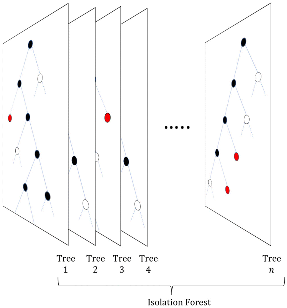 | ||
| Fig. 2 Isolation Forest architecture. A collection of partition trees combine to form a forest of trees, which are then used to detect data outliers (solid red nodes). Blue nodes that represent normal datapoints would be found much further down the tree and therefore are not shown. | ||
Once an Isolation Forest model has been trained, the measure of normality for each observation is determined as the average depth of the leaf containing the observation across the forest. The average pathlength (score 0.00 in Fig. 3) for data observations is used as a measure of normality, allowing for the detection of anomalies within a dataset. As such, a positive score will denote a longer pathlength (and therefore an indication of belonging to the normal group) and a negative score will denote a shorter pathlength (and therefor an indication of belonging to the outlier group). A decision threshold can then be employed to determine whether any new datapoints will be classified as an outlier or not, based on this score (see Fig. 3). This is the fundamental principle of the IF method.
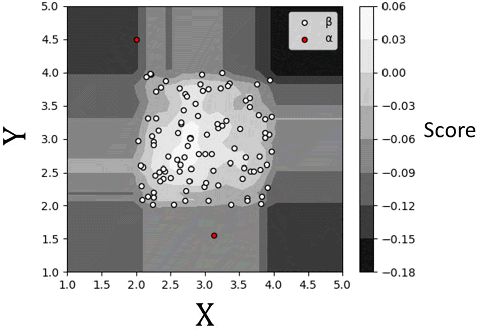 | ||
| Fig. 3 A scores plot representing the Isolation Forest algorithm decision criteria for detecting outliers. The score is a representation of a datapoint's pathlength relative to the average depths of the trees within the forest. A positive score denotes datapoints that have an average pathlength larger than the average tree depth, with a negative score denoting datapoints with shorter pathlengths. The lower the score, the more likely it is an outlier. | ||
Materials
The mouse livers used in this study were provided by the agrochemical company Syngenta, from a repeat dose, 14 day mouse study, investigating the impact of dietary exposure to an agrochemical. All experimental protocols used in this study were carried out in accordance with relevant standard operating procedures, including ethical and good laboratory practice (GLP) guidelines (home office number PPL 70/8624, toxicology of chemicals, protocol 2). The mouse livers were collected after 14 days. Twelve samples were used in this study, with equal numbers of male and female mice (three mice per dose group per sex), divided evenly across control and treatment groups. In this study only the control and high dose liver samples were used, totalling 12 liver samples.Sample preparation
Tissue samples were cut in paired sections for microscopy and spectroscopy applications respectively. All neutral buffered formalin-fixed and paraffin embedded (FFPE) liver samples were sectioned with two sequential tissue cuts from each liver paraffin wax block at a thickness of 5 μm. Tissues were prepared for Fourier-transform infrared spectroscopy (FT-IR) by mounting onto calcium fluoride (CaF2) slides and these tissues were left unstained and were not dewaxed. The samples were not dewaxed to mitigate against the effects of Resonance Mie scattering.18 Although scattering correction algorithms are available,19–21 it is often better to eliminate the scattering at source. This can be achieved by leaving the tissue in wax. The spectra then need only mild correction which can be achieved using simple baseline correction methods.22,23 The matched sequential sections were fixed in 10% neutral buffered formalin, haematoxylin and eosin (H&E)-stained, and loaded onto glass microscope slides. These samples were then sent for examination by a pathologist for treatment related findings and background lesions using a light microscope, with tissue abnormalities graded from minimal to severe using standardised grading protocols.24 The H&E-stained tissues were then scanned and digitised using a standard slide scanner.Infrared spectroscopy measurements
The Fourier-transform infrared spectroscopy (FT-IR) measurements were taken using an Agilent Cary 670-IR spectrometer coupled to an Agilent Cary 620-IR imaging microscope, fitted with a liquid nitrogen cooled mercury cadmium telluride (MCT), focal plane array (FPA) detector with 128 × 128 detector elements. The microscope was used with a 15× Cassegrain objective. The field-of-view produced by the instrument measured 704 × 704 μm, with each pixel measuring 5.5 × 5.5 μm. The sample stage and optics of the instrument were fitted within a sealable enclosure and provided with a continuous supply of dry air. Data were acquired at a relative humidity level of <1% to remove any water vapour from the compartment that could have been recorded as part of the sample spectrum. Prior to any sample scan, background scans were collected from a clean paraffin-free section of the CaF2 slide at a single FPA tile size consisting of 256 co-added scans at a spectral resolution of 5 cm−1. When scanning tissue sections, chemical images were obtained as collections of mosaics of multiple tiles in varying quantities ranging from 60 to over 120 tiles, consisting of 100 co-added scans; each tile scan taking approximately four minutes to acquire. Scans were performed in this manner due to the relative size of the tissue segments, with some tissue sections measuring 20 × 4 mm. Happ-Genzel interferogram apodisation was used with two levels of zero filling, with a spectral range of 900 to 3800 cm−1.Data pre-processing
All data analysis was performed in the Python programming language (version 3.9) using Spyder.25 To separate tissue spectra from that of paraffin wax, infrared spectra for each sample were extracted from the mosaic through unsupervised k-means clustering of the area under the amide I and II bands between 1500–1700 cm−1. Tissue fragments or breakaway tissue sections were then removed using a segmentation approach using skikit-image which kept the largest regions of tissue in descending order until 95% of all tissue was captured.26 The signal-to-noise ratio of the raw spectra extracted were then improved using principal components-based noise reduction with the first 60 principal components being retained. This selection was made following the application of multiple calculations of the Predicted Residual Error Sum of Squares (PRESS) to Residual Sum of Squares (RSS) ratio (PRESS/RSS) across multiple samples to determine the general number of significant principal components that explains the acquired datasets.27 The calculated metric did not surpass 25 principal components, meaning there is confidence that 60 principal components for smoothing are sufficiently large so as not to remove any components related to chemical information.The spectra were restricted to the 950–1850 cm−1 wavenumber region, with the wavenumber regions associated with paraffin wax at 1350–1480 cm−1 being removed. Normalisation was conducted using vector normalisation of the remaining spectra. The first derivative of the data were then computed using the Savitzky–Golay (SG) method to reduce contribution from broad and structureless elements,13,28 with a window size of 13 data points and a 4th order fitted polynomial. Following derivative calculation, spectral artefacts introduced by edge effects in the SG method are removed, with these data restricted to the 1000–1800 cm−1 wavenumber region and removal of data between 1340–1490 cm−1. This order was followed to avoid any contribution of wax peaks in the normalisation of data. Finally, to allow for better random partitioning of the methods employed in this study, the derivative data was scaled by a factor of 1 × 10⁶, due to rounding errors caused by the original data scale following derivative conversion.
Hardware specifications
The analyses were conducted with the following relevant hardware components:• Processor: 28 core Intel(R) Xeon(R) W-2275 CPU @ 3.30 GHz.
• Installed RAM: 128GB.
• GPU: NVIDIA Quadro RTX 6000 24GB GDDR8 with 4608 CUDA cores.
Model predictions were conducted at the whole tissue level. Given these datasets ranged from 6–12 GB in size, conducting the same analyses on hardware with less physical memory might not be possible due to physical memory limitations. In these instances, memory mapping/chunking methods may be a viable approach.
The full process of model training took approximately 46 minutes per model and full sample predictions took approximately 1 hour per sample. These large run times are mainly taken up by the loading and handling of the data, caused by the large number of spectra in each sample (∼3 million spectra per sample). Comparatively, the actual training of the IF model following sampling is much faster, only taking 28 seconds.
The average time to make predictions on 100![[thin space (1/6-em)]](https://www.rsc.org/images/entities/char_2009.gif) 000 spectra (following loading and handling) was 1 minute and 48 seconds.
000 spectra (following loading and handling) was 1 minute and 48 seconds.
Model training
Model building and training was completed in the Python programming language (version 3.9) utilising the scikit-learn package.25,29 Models were trained for male and female liver samples separately. The decision to separate by sex was determined by the differences in tissue chemical structure and variations associated with male and female liver functions such as differences in glycogen synthase following feeding and differences in oestradiol.30 Model training was conducted on the first derivative data of control samples hepatocytes (which make up the majority of tissue in the liver) as outlined in the pre-processing section. To capture the variation across the control mice samples, random sampling was conducted individually across each sample to ensure even group sizes. For each sex, three specimen samples were used in model training with three samples used for testing. Training sets were built by randomly sampling 5000 spectra from each of the three control training samples, making 15000 spectra in total. Model specific parameters can be found in Table 1. It is important to note that the same pre-processing and model training protocol is followed for each of the male and female animal liver models.
| Model | Number of spectra | Model parameters |
|---|---|---|
| Isolation forest | 15000 |
n_estimators = 600 |
| max_samples = 3000 | ||
| Contamination = ‘auto’ | ||
| Bootstrap = true |
Results
Having built a model on the control samples, the anomaly detection method was applied to three male and three female agrochemical-dosed mice liver samples across twenty-one datasets totalling 8380102 male and 7280080 female liver spectra. The differences between the size of the normal and abnormal spectral counts can be found in Table 2. These samples contained instances of abnormal tissue not observed in the control training tissue, including interferents. The model classified independent spectra in to “normal” and “abnormal” groups (1 and −1 labels). In the case of this study, the group “normal” refers to the healthy hepatocytes that were used in the training of the model, with “abnormal” referring to all things not belonging to that group. While other groups found in tissue such as blood vessels and arterioles are not biological anomalies, they are defined as anomalous compared to the defined “normal” class in this study. These definitions of “normal” and “abnormal” will vary depending on the framing of the problem space the method is being applied to and should be well defined in each instance by future users.
| Sample | Number of test spectra | Number of test spectra identified as normal | Number of test spectra identified as anomalous (not normal) | Percentage of anomalous spectra |
|---|---|---|---|---|
| Male 1 | 2870512 |
2367544 |
502968 |
18% |
| Male 2 | 2597729 |
2174343 |
423386 |
16% |
| Male 3 | 2911861 |
2605401 |
306460 |
11% |
| Female 1 | 2633463 |
2547243 |
86220 |
3% |
| Female 2 | 2185714 |
2002992 |
182722 |
8% |
| Female 3 | 2460903 |
2370694 |
90209 |
4% |
To determine if the model is identifying statistically significant differences between the groups, the Kruskal–Wallis non-parametric one-way analysis of variance test was applied to the data groups segmented by the method.31,32 This test was applied to the first derivative data. The Kruskal–Wallis test determines the independence of distributions and was conducted at every wavenumber between both identified groups for every FTIR dataset at the one percent significance level (p-value = 0.01). For both male and female results shown in Fig. 4 wavenumber positions are highlighted where the test-statistic result fails to reject the null hypothesis of groups belonging to the same distribution in a single dataset or more in the test applied to the first derivative data. The results indicate that the groups identified by the IF method ultimately have independent distributions for the majority of wavenumber readings, and that even when considering all tests it can be said that the IF method is identifying anomalous data to a statistically significant degree.
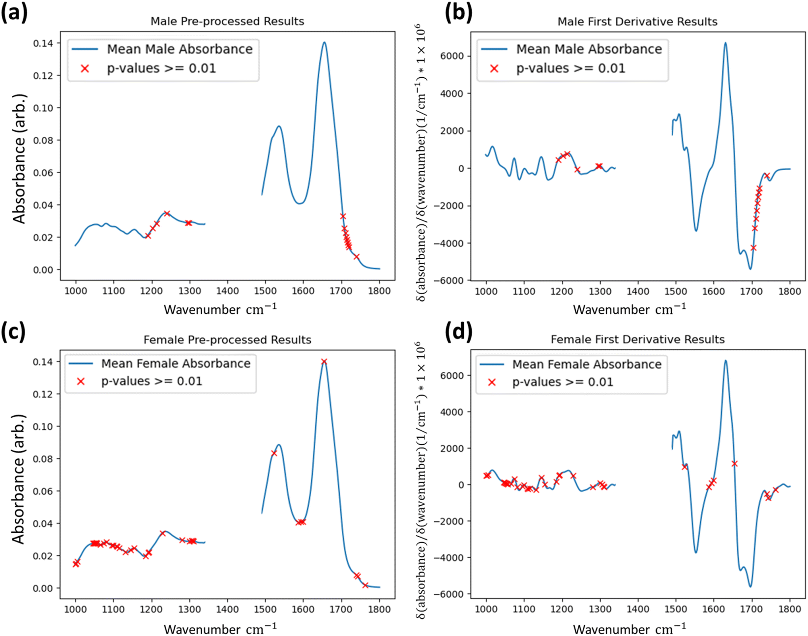 | ||
| Fig. 4 Wavenumbers of non-independence (red crosses) between the two groups returned by the Isolation Forest identified by the Kruskal–Wallis test at a 1% significance level. Regions of non-independence are overlaid to the mean spectrum (solid blue line) of the pre-processed and first derivative plots of both male (a and b) and female (c and d) spectral datasets. | ||
Further insight can be gained by retrospective unsupervised k-means clustering of the first derivative spectra for returned data that are labelled as “anomalous” by the IF technique (3 and 4 clusters, default remaining parameters29), serving to show how the method is capturing spectra with both clear and subtle differences to the overall tissue average, as shown in Fig. 5.
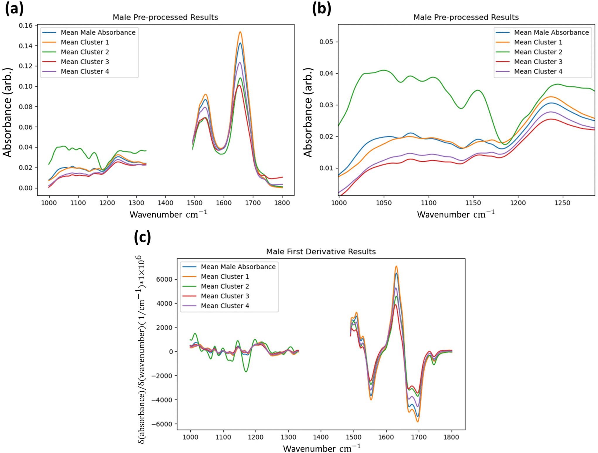 | ||
| Fig. 5 Mean absorbance of groups of spectra being identified as anomalous by the IF method from a single sample set following pre-processing, but without calculation of the first derivative in the full fingerprint region (a) with focus on the lower wavenumber region (b), alongside results in the first derivative (c). The overall tissue mean is plotted for comparison. | ||
Discussion
The results of the Kruskal–Wallis tests applied to the returned datasets shows that non-normal tissue constituents are being identified by the Isolation Forest algorithm. However, non-normal tissue constituents comprise of many different categories/causes, including tissue and non-tissue examples. Additionally, there appear to be differences in the sex-specific results. As such, the models’ outputs and the underlying datasets warrant discussion to understand better how this technique operates.In the agrochemical study from which the sample sets were obtained only the male liver samples contained instances of non-neoplastic lesions of hepatocellular necrosis. This difference in biology, compared to the female mice, is evidenced in the number of spectra identified as being abnormal in Table 2. In total, there are many fewer anomalous data found in the female liver samples compared to the males, implying there are inter-sex related differences between the two sets of data. It is known that biological differences in hormone levels and metabolic activity exist between male and female mice, resulting in different organ response and effect of xenobiotic exposure.30,33–35 This could account for the differences in Kruskal–Wallis test results across the wavenumber ranges highlighted in Fig. 4, alongside the difference in total spectra being identified as anomalous.
With regards to the detection of anomalous data, histopathological assessment of anomaly outputs implies that the IF method can identify spatial regions where necrosis may be evident as in Fig. 6, amongst other identified features. Analysis of the identified spectra in the regions marked necrotic in the adjacent H&E sections further confirm the identification of the necrotic hepatocytes, as shown in Fig. 6, with clear deformation of glycogen and phosphodiester peaks correlating with a rise in suspected tyrosine protein kinase, all indicators of a dying cell.36–39 This finding indicates that the method can correctly discriminate between hypertrophic cells (which are a normal biological process) and the necrotic cells, which have subtle differences in their spectra. This is shown in the ESI.† Beyond the identification of tissue lesions, the IF approach can identify additional tissue constituents. As shown in Fig. 7, a large region of connective tissue, bile ducts, inflammatory cells and arterioles have been identified as anomalous data, which is correct given the IF model is trained solely on healthy hepatocytes. Spectrally these constituents are grouped similarly when utilising k-means clustering, possibly due to pixel mixing (pixels that have contribution from multiple sources, such as wax and tissue all within the same 5.5 × 5.5 μm pixel region) but are clearly different enough from the normal tissue spectral absorbance patterns. Beyond other tissue constituents that are biologically relevant, the anomaly detection algorithm can also indicate interferents such as dust or hair particles that have found their way on to the sample itself prior to scanning. These can be identified visually in the sample scans due to the high intensity of absorbance, and distinctly different spectral absorbance profiles. Examples of this can be found in the ESI.† The anomaly detection method can also find damaged tissue and mixed pixels at the sample edges that have partial contribution from both tissue and non-tissue parts, highlighting the broad scope of the anomaly detection method, allowing for a quality control function. This is also shown in the ESI.† These mixed pixels are characterised by their lower signal intensity of biologically relevant spectral features and increased paraffin peak signal and can be identified at the boundary of venular portals, torn tissues, and the boundary between tissue and the embedding paraffin.
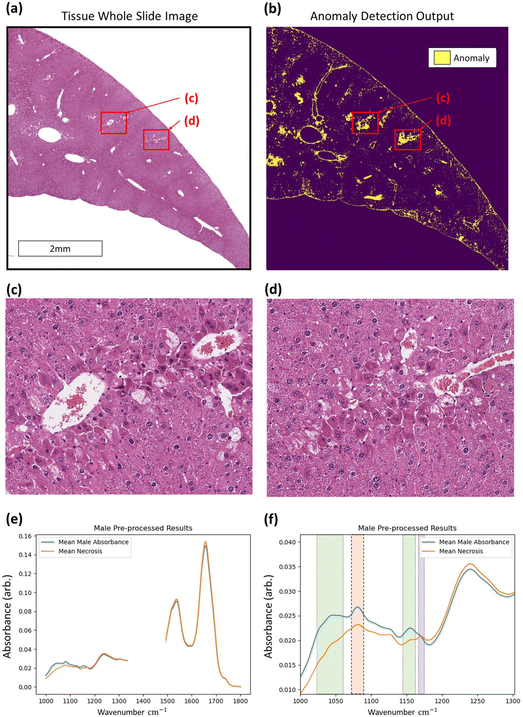 | ||
| Fig. 6 Identification of non-neoplastic lesions using the anomaly detection method. Regions of hepatocellular necrosis seen in the whole slide image of a mouse liver (a) correspond to those identified by the anomaly detection output (b). Example regions (c and d respectively) indicate a correlation between the IF results and pathological insight. Confirmation of method capture of non-neoplastic lesions (hepatocellular necrosis) is confirmed by plotting the mean absorbance profile of pre-processed spectra for an entire tissue section (blue) and identified necrosis (orange). The fingerprint region without wax peaks (a) and lower wavenumber region (b) are plotted, highlighting wavenumber regions of glycogen (green rectangles), phosphodiester (orange rectangle), and tyrosine-protein kinase (purple rectangle) content. | ||
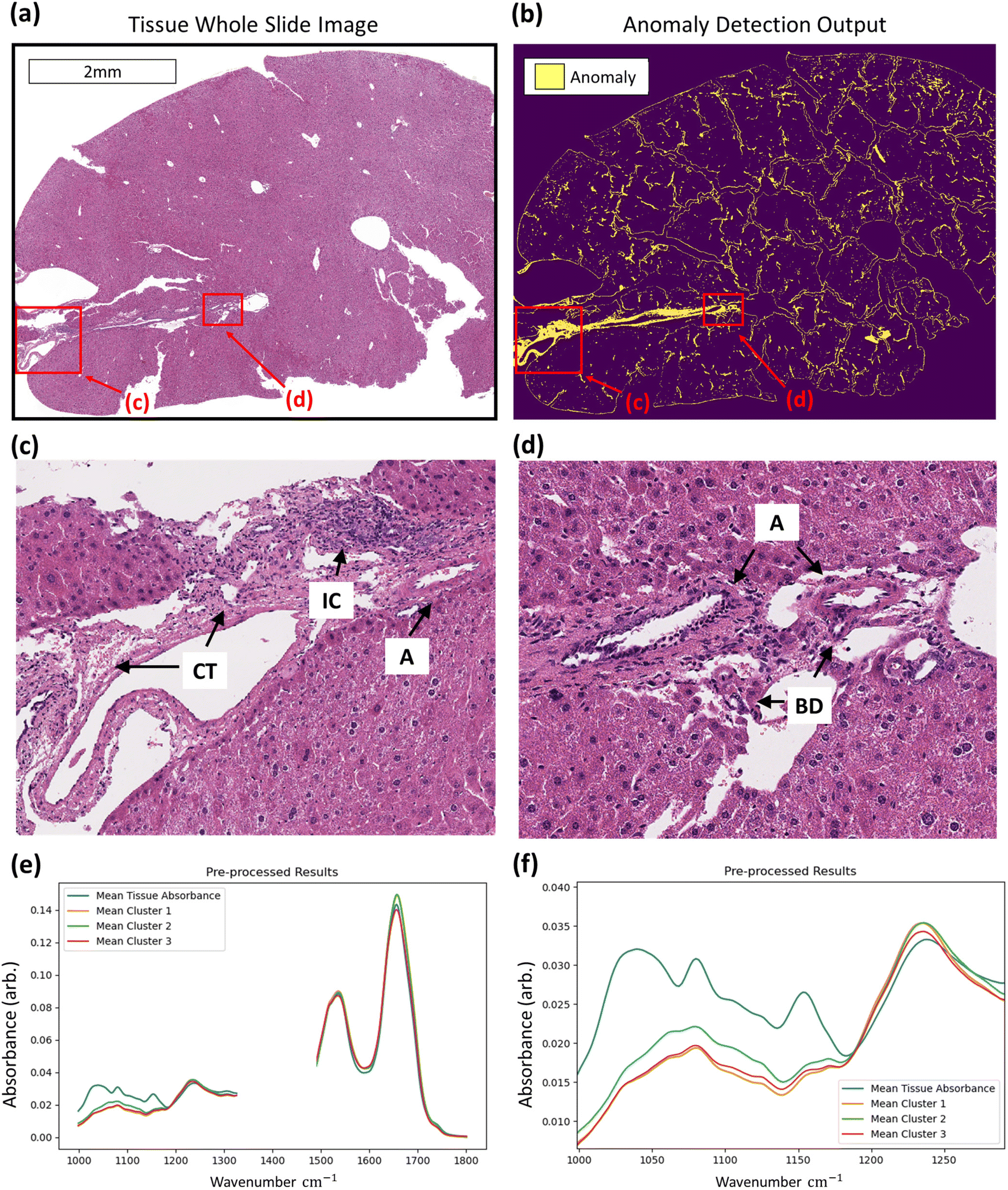 | ||
| Fig. 7 Identification of additional tissue constituents using the anomaly detection method. Regions of interest in the whole slide image of tissue (a) are highlighted (red boxes) where the anomaly detection method output (b) has identified regions of non-normal tissue. These regions (c and d respectively) show captured regions of connective tissue (CT), inflammatory cells (IC), arterioles (A), and bile ducts (BD). Confirmation of method capture of different tissue constituents is confirmed through plotting the mean absorbance profile (solid colour lines) of pre-processed spectral groups for an entire tissue section (blue) against k-means clusters of identified anomalies matched to additional tissue constituents (orange, green, and red). The fingerprint region without wax peaks (e) and lower wavenumber region (f) are plotted. | ||
Conclusions
The novel method of weakly supervised anomaly detection is able to detect abnormal FT-IR spectra collected from mouse liver tissue, capturing multiple instances of anomalous data, with ‘anomalous’ implying any non-normal healthy hepatocellular tissue: non-neoplastic lesions such as hepatocellular necrosis, alternative tissue constituents such as connective tissue, bile ducts, arterioles, and inflammatory cells, interferents such as dust or hair, folded tissue, and damaged tissue. This was achieved by building a model solely from a small subsample of control liver tissue data containing healthy hepatocytes only. The groups captured by this method have statistically significant differences in their wavenumber absorbances across all sample sets using the Kruskal–Wallis test of independence, with pre-processed and first derivative absorbance profiles of these groups highlighting the key differences.The implications of these results are that anomaly detection of FT-IR spectra could become a new method of classification available to researchers working with tissue with no readily available labelled groups, or for those attempting to detect anomalous data for quality control purposes within homogenous tissue types, or groups of data with low occurrence rates. Additional implications of this method are its potential implementation within regulatory animal toxicity studies. Researchers could feasibly develop an anomaly detection methodology from immediately available control sample data, analysing tissue data as they become available. For relatively homogenous tissue samples, models trained on control/healthy datasets could feasibly be transferred to multiple disease/lesion classification problems. This in turn can decrease the amount of control data requiring generation for tissue studies, with a repository or databank of known “normal” data. This would bring about cost and time savings. Additionally, this would allow toxicologic pathologists to concentrate on unusual or minimal findings in treated animals (traditionally difficult to identify), instead of spending valuable time identifying background findings in control tissues, improving their workflows.
Author contributions
Dougal Ferguson: conceptualization, methodology, formal analysis, investigation, writing – original draft, visualization. Alex Henderson: conceptualization, supervision. Elizabeth F. McInnes: writing – review & editing, supervision. Peter Gardner: conceptualization, writing – review & editing, supervision.Data availability
The ownership and associated rights for the data used in this publication belong to Syngenta. The software implemented in this study are available as open-source packages and found in their relevant citations.Conflicts of interest
The authors of this paper declare no conflicts of interest.Acknowledgements
Partial funding is provided by a block grant from the Engineering and Physical Sciences Research Council (EPSRC) and additional funding is provided by Syngenta AG. The authors also acknowledge Charles River Laboratories for the supply of relevant study samples. We also thank the Williamson Trust for generous support for the purchase of the infrared microscope. We gratefully thank Mr Stuart Naylor (Charles River Laboratories, Elphinstone, Tranent) for the preparation of histologic sections.References
- B. C. Smith, Fundamentals of Fourier transform infrared spectroscopy, CRC press, 2011 Search PubMed.
- M. J. Baker, J. Trevisan, P. Bassan, R. Bhargava, H. Butler, K. M. Dorling, P. R. Fielden, S. W. Fogarty, N. J. Fullwood, K. Heys, C. Hughes, P. Lasch, P. L. Martin-Hirsch, B. Obinaju, G. D. Sockalingum, J. Sulé-Suso, R. Strong, M. J. Walsh, B. R. Wood, P. Gardner and F. L. Martin, Nat. Protoc., 2014, 9, 1171 CrossRef PubMed.
- M. Piling and P. Gardner, Chem. Soc. Rev., 2016, 45, 1935–1957 RSC.
- M. J. Baker, H. J. Byrne, J. Chalmers, P. Gardner, R. Goodacre, A. Henderson, S. G. Kazarian, F. L. Martin, J. Moger, N. Stone and J. Sulé-Suso, Analyst, 2018, 143, 1735–1757 RSC.
- C. A. Meza Ramirez, M. Greenop, L. Ashton and I. U. Rehman, Appl. Spectrosc. Rev., 2020, 56(8–10), 733–763 Search PubMed.
- I. U. Rehman, R. S. Khan and S. Rehman, Expert Rev. Mol. Diagn., 2020, 20, 749–755 CrossRef CAS PubMed.
- J. Tang, A. Henderson and P. Gardner, Analyst, 2021, 146, 5880–5891 RSC.
- F. Großerueschkamp, T. Kallenbach-Thieltges, T. Behrens, T. Brüning, M. Altmayer, G. Stamatis, D. Theegarten and K. Gerwert, Analyst, 2015, 140, 2114–2120 RSC.
- C. Kuepper, F. Großerueschkamp, A. Kallenbach-Thieltges, A. Mosig, A. Tannapfel and K. Gerwert, Faraday Discuss., 2016, 187, 105–118 RSC.
- G. Theophilou, K. M. Lima, P. L. Martin-Hirsch, H. F. Stringfellow and F. L. Martin, Analyst, 2016, 141, 585–594 RSC.
- K. Chrabaszcz, K. Kochan, A. Fedorowicz, A. Jasztal, E. Buczek, L. S. Leslie, R. Bhargava, K. Malek, S. Chlopicki and K. M. Marzec, Analyst, 2018, 143, 2042–2050 RSC.
- S. Mittal, T. P. Wrobel, M. Walsh, A. Kajdacsy-Balla and R. Bhargava, Clin. Spectrosc., 2021, 3, 100006 CrossRef.
- D. Ferguson, A. Henderson, E. F. McInnes, R. Lind, J. Wildenhain and P. Gardner, The Analyst, 2022, 147(16), 3709–3722 RSC.
- Y. Liu, H. H. Zhang and Y. Wu, J. Am. Stat. Assoc., 2010, 106, 166–177 CrossRef PubMed.
- F. T. Liu, K. M. Ting and Z. H. Zhou, IEEE, 2008, 413–422 CAS.
- F. T. Liu, K. M. Ting and Z. H. Zhou, ACM Transactions on Knowledge Discovery from Data (TKDD), 2012, vol. 6, pp. 1–39 Search PubMed.
- T. G. Dietterich, Ensemble methods in machine learning. InInternational workshop on multiple classifier system, Springer, Berlin, Heidelberg, 2000 Search PubMed.
- P. Bassan, H. J. Byrne, F. Bonnier, J. Lee, P. Dumas and P. Gardner, Analyst, 2009, 134, 1586–1593 RSC.
- P. Bassan, A. Kohler, H. Martens, J. Lee, H. J. Byrne, P. Dumas, E. Gazi, M. Brown, N. Clarke and P. Gardner, Analyst, 2010, 135, 268–277 RSC.
- P. Bassan, A. Kohler, H. Martens, J. Lee, E. Jackson, N. Lockyer, P. Dumas, M. Brown, N. Clarke and P. Gardner, Biophotonics, 2010, 3, 609–620 CrossRef CAS PubMed.
- E. A. Magnussen, J. H. Solheim, U. Blazhko, V. Tafintseva, K. Tøndel, K. H. Liland, S. Dzurendova, V. Shapaval, C. Sandt, F. Borondics and A. Kohler, J. Biophotonics, 2020, 13, e202000204 CrossRef CAS PubMed.
- P. Bassan, A. Sachdeva, J. H. Shanks, M. D. Brown, N. W. Clarke and P. Gardner, Medical Imaging 2014: Digital Pathology, 2014, vol. 9041, pp. 83–92 Search PubMed.
- P. Bassan, J. Mellor, J. Shapiro, K. J. Williams, M. P. Lisanti and P. Gardner, Anal. Chem., 2014, 86, 1648–1653 CrossRef CAS PubMed.
- C. L. Scudamore, Practical approaches to reviewing and recording pathology data, Wiley Blackwell, 2014 Search PubMed.
- P. Raybaut, Spyder-documentation, 2009.
- S. Van Der Walt, J. L. Schönberger, J. Nunez-Iglesias, F. Boulogne, J. D. Warner, N. Yager, E. Gouillart and T. Yu, PeerJ, 2014, 2, e453 CrossRef PubMed.
- R. G. Brereton, Chemometrics for pattern recognition, John Wiley & Sons, 2009 Search PubMed.
- P. A. Gorry, Anal. Chem., 1990, 62, 570–573 CrossRef CAS.
- F. Pedregosa, G. Varoquaux, A. Gramfort, V. Michel, B. Thirion, O. Grisel, M. Blondel, P. Prettenhofer, R. Weiss, V. Dubourg and J. Vanderplas, J. Mach. Learn. Res., 2011, 12, 2825–2830 Search PubMed.
- P. M. Treuting, S. Dintzis and K. S. Montine, Comparative anatomy and histology: a mouse, rat, and human atlas, Academic Press, 2017 Search PubMed.
- W. H. Kruskal and W. A. Wallis, J. Am. Stat. Assoc., 1953, 48, 907–911 CrossRef.
- T. W. MacFarland and J. M. Yates, Introduction to Nonparametric Statistics for the Biological Sciences Using R, Springer, Cham, 2016, pp. 177–211 Search PubMed.
- V. Wauthier, A. Sugathan, R. D. Meyer, A. A. Dombkowski and D. J. Waxman, Mol. Endocrinol., 2010, 24, 667–678 CrossRef CAS PubMed.
- X. Yang, E. E. Schadt, S. Wang, H. Wang, A. P. Arnold, L. Ingram-Drake, T. A. Drake and A. J. Lusis, Genome Res., 2006, 16, 995–1004 CrossRef CAS PubMed.
- J. N. MacLeod, N. A. Pampori and B. H. Shapiro, J. Endocrinol., 1991, 131, 395–399 CAS.
- Z. Movasaghi, S. Rehman and D. I. ur Rehman, Appl. Spectrosc. Rev., 2008, 43, 134–179 CrossRef CAS.
- V. Zohdi, D. Whelan, B. Wood, J. T. Pearson, K. R. Bambery and M. J. Black, PLoS One, 2015, 10(2), e0116491 CrossRef PubMed.
- P. T. Wong, E. D. Papavassiliou and B. Rigas, Appl. Spectrosc., 1991, 45, 1563–1567 CrossRef CAS.
- P. T. Wong, R. K. Wong, T. A. Caputo, T. A. Godwin and B. Rigas, Proc. Natl. Acad. Sci. U. S. A., 1991, 88, 10988–10992 CrossRef CAS PubMed.
Footnote |
| † Electronic supplementary information (ESI) available. See DOI: https://doi.org/10.1039/d3an00618b |
| This journal is © The Royal Society of Chemistry 2023 |