Accurate predictions of thermoset resin glass transition temperatures from all-atom molecular dynamics simulation

Abstract

To enable the design and development of the next generation of high-performance composite materials, there is a need to establish improved computational simulation protocols for accurate and efficient prediction of physical, mechanical, and thermal properties of thermoset resins. This is especially true for the prediction of glass transition temperature (T_g), as there are many discrepancies in the literature regarding simulation protocols and the use of cooling rate correction factors for predicting values using molecular dynamics (MD) simulation. The objectives of this study are to demonstrate accurate prediction the T_g with MD without the use of cooling rate correction factors and to establish the influence of simulated conformational state and heating/cooling cycles on physical, mechanical, and thermal properties predicted with MD. The experimentally-validated MD results indicate that accurate predictions of T_g, elastic modulus, strength, and coefficient of thermal expansion are highly reliant upon establishing MD models with mass densities that match experiment within 2%. The results also indicate the cooling rate correction factors, model building within different conformational states, and the choice of heating/cooling simulation runs do not provide statistically significant differences in the accurate prediction of T_g values, given the typical scatter observed in MD predictions of amorphous polymer properties.

---

Introduction

High-performance thermoset composites are the primary structural material used in modern aircraft and aerospace materials. Their high specific modulus and specific strength are critical for reduced fuel costs. There is an ongoing need to develop improved thermoset resins and composite processing methods to further improve composite mechanical properties and provide more cost-efficient and effective manufacturing methods. Computational simulation can be used to efficiently drive the design of future generations of thermoset resins, composites, and processing methods. Specifically, Molecular Dynamics (MD) simulation can be used to accurately and efficiently predict the influence of molecular structure on bulk physical, mechanical, and thermal properties of high-performance thermoset resins.^1–13 This capability is necessary for establishing structure–property relationships, providing physical insight into observed behavior, and enabling the bottom-up design and analysis of thermoset composites.

Like all amorphous materials, thermoset resins exhibit a glass transition temperature (T_g) that separates the rubbery and glassy material responses. The physical, mechanical, and thermal responses of a thermoset resin change dramatically as the material is either heated or cooled through the T_g. It is well-known that experimental measurements of T_g are highly affected by cooling rates.^14–18 Under laboratory conditions, rapid cooling through the T_g window does not provide the polymer molecular structure enough time to respond to rapid reductions in free volume via chain segment conformational changes. As a result, non-equilibrium conformations are locked in, which contain more free volume than conformations resulting from slower cooling. Such T_g measurements from rapid cooling provide an apparent T_g that is higher than those observed with slower cooling. The dependence of T_g on cooling rate presents a particular concern with MD simulation, where the simulated cooling rates are up to ten orders of magnitude larger than those used under laboratory conditions.

Numerous studies have investigated MD methods for predicting the T_g of thermoset resins.^{1–4,8,9,13,19–38} Some of these studies^{1,3,22,23,29,38} employ a cooling rate correction factor to correct the predicted values of T_g to match those measured under laboratory conditions with much slower cooling rates. Specifically, the well-established Williams–Landel–Ferry equation^39,40 has been used to reduce the apparent predicted T_g by about 3 K per decade of cooling rate (about 30 K for most MD simulations). However, careful examination of the complete set of above-cited papers using MD to predict T_g of thermosets show an inconsistent trend in predictions. While many of the papers show predictions that overestimate the measured values of T_g, the magnitude of overprediction varies greatly, while some papers show a close match or an underprediction of T_g. The papers also report predicted mass densities that vary greatly in accuracy compared to experimental measurements, which is problematic since the T_g is critically dependent on the mass density of the thermoset.¹⁷ The cause of the inconsistent agreement in mass density and T_g with experiment could be related to modelling techniques and the use of inadequate force fields.

Recently, Odegard et al.⁴ used the reactive Interface Force Field (IFF-R)⁴¹ to show that with the prediction of mass densities that match experiment within 0.014 g cc⁻¹ and well-parameterized force constants, T_g values can be predicted with MD that closely match experiment for both heating and cooling, without using any correction factors. Clearly, there is a further need to understand the accurate prediction of T_g with MD, and carefully examine the necessity of using correction factors to match experimentally-measured values.

The first objective of this study is to demonstrate accurate prediction the T_g of two thermosets with MD without the use of cooling rate correction factors. The second objective is to establish the influence of simulated conformational state and heating/cooling cycles on physical, mechanical, and thermal properties predicted with MD. The theories of the glass transition, polymer conformational state, and free volume is reviewed, followed by a description of the MD simulations performed herein. The MD modelling results are compared to experiment for validation, and analysed to provide physical insight into the process of simulating thermosets for accurate prediction of physical, mechanical, and thermal properties.

Physics of MD modelling of the glass transition

The free volume in a polymer is commonly defined as the volume that is not occupied by polymer molecules or other chemical compounds, including gas molecules. With this definition, a quantitative measurement of free volume is complicated by the ambiguous definition of the volume of the atoms in the system. However, for the purposes of this discussion, this definition will be sufficient. In general, as the temperature of a thermoset network increases, the thermal oscillation of the atoms will also increase, and network segments will naturally push each other away. This action increases the free volume of the material, and manifests itself in a bulk-level thermal expansion. The reverse action occurs when the network temperature decreases. Changes in free volume in response to temperature changes are relatively fast, that is, on typical all-atom MD time scales.

A conformational change in a polymer network corresponds to a chain segment rotation, twist, or angle change, and is driven by thermal oscillations and the necessity to minimize conformational energy relative to the amount of free volume available. Therefore, there is an ideal conformation for every chain segment at a given temperature, as dictated by the van der Waals forces between neighbouring chain segments and the topology of the chain segments. As the network temperature changes, the corresponding free volume will change, and a thermodynamic driving force for conformational changes will arise. In general, conformational changes occur at a wide range of time scales spanning nanoseconds to years (a.k.a. physical aging¹⁷) due to steric hindrance from neighbouring segments. Given enough time, a thermoset network at a constant temperature will slowly be driven to a conformational equilibrium, which is uniquely dependent on the temperature.

At elevated temperatures, the free volume in the thermoset network is substantial and allows conformational changes to easily occur. In this rubbery state (Fig. 1, State A), conformational changes can occur within minutes. In the rubbery state, any locked-in conformations that were created during a preceding cool-down step can be released so that the conformational state can quickly reach the equilibrium that corresponds to the elevated temperature (a.k.a. rejuvenation¹⁷). Because of the high levels of free volume, the rubbery state is associated with a lower stiffness and high coefficient of thermal expansion.

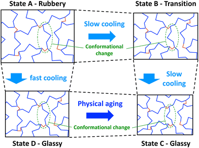Fig. 1 Simplified 2D schematic showing conformational transitions of a thermoset network during cooling (monomers in blue and crosslinks in red).

If the network in the rubbery state is cooled slowly, conformational changes can occur to accommodate the reductions in free volume to keep the network in equilibrium (Fig. 1, State B). If slow cooling continues to relatively low temperatures, low levels of free volume (thus high levels of steric hindrance) severely slow down the conformational change process. In this glassy state (Fig. 1, State C), the thermoset chain segments adopt conformations that accommodate the reduced volume. Because of the higher levels of mass density of the glassy state, higher values of stiffness and lowers levels of thermal expansion are typically observed.

If the network is cooled from the rubbery state relatively quickly, the free volume of the network will also decrease quickly, but the slower conformational changes will not be able keep up with the decreasing volume, and the resulting increase in steric hindrance will “lock in” a non-equilibrium conformation (Fig. 1, State D). An apparent glassy state is obtained, which has higher levels of free volume than the glassy state that is obtained with slow cooling (Fig. 1, State C). Because the glassy states have two different mass densities, they are expected to have different thermal and mechanical properties. Eventually, through physical aging, the rapidly-cooled glassy state will slowly experience physical aging that eventually bring it to the glassy state that is obtained with slow cooling.

The reversable transition from the glassy state to the rubbery state (and vice versa) occurs over the glass transition window, but is typically (and herein) referenced as the singular scalar value T_g. Physically, the T_g corresponds to the apparent temperature at which the drive for conformational changes is equal to the resistance to such changes from steric hindrance, which is in turn driven by the constraining forces associated with free volume and thermal expansion/contraction. Different thermosets have different T_g values because of the different sizes, morphologies, and stiffnesses of the chain segments.

When cooling from the rubbery to glassy states, the rate of cooling dictates the observed T_g (Fig. 2). If the cooling is slow enough (Fig. 2, States A–C), the system will be in continual equilibrium through the T_g. That is, the chain conformation will always be in equilibrium (Fig. 1, States A–C). The thermal contraction will eventually eliminate enough free volume such that further chain motion is critically reduced, leading to a sudden reduction in further thermal contraction (Fig. 2, State B). This results in the lowest possible value of T_g, known as the fictive temperature, T_f. A thermoset in this state will have its highest mass density relative to the temperature. If the cooling rate (q₁) is too fast (Fig. 2, States A–D), conformational changes cannot occur on pace with the reductions in free volume from thermal contraction. The constraining forces from thermal contraction thus lock in the lower density conformational state (Fig. 1, State D), and the thermal contraction is prematurely reduced, leading to higher observed T_g. At this point, the conformational state is no longer in equilibrium. A thermoset in this state will have a lower mass density than it would if it were equilibrium. Eventually, the system will be driven to equilibrium via long-term physical aging (Fig. 1 and 2, States D–C).

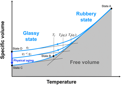Fig. 2 Specific volume (inverse of mass density) versus temperature for a fully crosslinked thermoset. The labelled states correspond to those depicted in Fig. 1.

It should now be apparent that any attempt to use all-atom MD modeling to simulate the actual transition from a rubbery to glassy state (or vice versa) is burdened with the computational limitation of nanosecond simulation times, as significant conformational changes may occur at much larger time scales. Thus, all-atom MD cannot directly simulate the A–B–C path shown in Fig. 1 and 2.

Although coarse-grain simulation techniques^42–46 can be used somewhat avert the time scale limitation, they require conversion between all-atom and coarse-grain geometries, and thus at least one extra step compared to all-atom simulations alone. Unfortunately, some of the fine (and perhaps critically important) details of atomic interactions are lost when converting to a coarse-grain simulation. Thus, this paper will henceforth only focus on all-atom simulations.

A common approach to build condensed all-atom MD models of thermoset monomers is to place the monomers in a large simulation box at a very low mass density, and slowly condense the box (to a target mass density) such that the monomers naturally densify together into the liquid state. This is followed by simulated crosslinking, which brings the simulated thermoset to its solid state. It is important to note that we will henceforth assume that the solid state mass density is within 0.014 g cc⁻¹ of the experimentally measured mass density,⁴ which is not consistently achieved with many of the MD modeling papers cited above, likely due to the use of inadequate force fields or poorly chosen target mass densities.

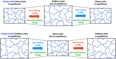
Now we will examine two scenarios. First, suppose that we build and crosslink an MD model below T_g (henceforth referred to as the glassy build), as shown in the top row of Fig. 3 (State C of Fig. 1 and 2). If we heat this model through the T_g, the free volume of the model can increase with the thermal expansion on MD timescales. However, conformational changes cannot be fully simulated with MD because they require much longer times scales, so the glassy build will likely be out of equilibrium above T_g. If that model is subsequently cooled below T_g, it is likely already trapped in a glassy conformation because of the MD/experimental time scale mismatch, so the corresponding predicted T_g will be close to the fictive temperature and experimentally-measured T_g values with very slow cooling rates.

Fig. 3 Two scenarios of building MD models of a thermoset and transitioning through the T_g.

Second, suppose that we build and crosslink an MD model of a thermoset above T_g (henceforth referred to as the rubbery build), as shown in the bottom row of Fig. 3 (State A of Fig. 1 and 2). If the model is cooled through the T_g, the rubbery conformation cannot completely adapt to the rapid cooling, and the rapid decrease in free volume will lock-in the rubbery conformation before the T_f is reached, thus prematurely causing the thermal contraction to drop. Thus, the apparent T_g will likely be above the T_f, and we may observe the cooling rate effect that is observed experimentally. If the model is subsequently heated back to the rubbery state, the rubbery conformation is already locked into the model, and the rapid increase associated with the rubbery thermal expansion may not be realized until the temperature has reached the relatively high apparent T_g.

These two simulation approaches provide us with an excellent opportunity to gain insight into the MD modelling process for predicting T_g and other temperature-dependent properties. In combination with the use of appropriate force fields and accurate mass densities, comparison of predicted results from these two approaches can establish the significance of the cooling rate effect in all-atom MD modelling.

Materials

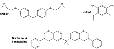
Two thermoset systems were considered in this study:

• Epoxy: Diglycidyl ether bisphenol F (DGEBF) epoxide monomer with an aromatic diethyltoluenediamine (DETDA) curing agent. This system is commercially manufactured as EPON 862/EPIKURE W.

• Polybenzoxazine (PBZ): Bisphenol A benzoxazine monomer. This system is commercially manufactured as Araldite 35600.

The molecular structures of the corresponding monomers are shown in Fig. 4.

Fig. 4 Epoxy (top) and PBZ (bottom) monomer molecular structures.

Simulation methods

The LAMMPS (Large-scale Atomic/Molecular Massively Parallel Simulator) software package⁴⁷ was used for all MD simulations described herein, utilizing the IFF-R force field. The virtual π orbitals that have been used previously with IFF^48–50 were not used in the current study because no aromatic reinforcement surfaces were simulated (e.g. graphene or carbon nanotubes). IFF-R has been previously shown to accurately predict physical, thermal, and mechanical properties of thermoset resins.^4,5,51 The Lennard-Jones diameters were chosen per guidelines described by Heinz et al.⁵² Nose–Hoover^53–55 algorithms were used for both the thermostats and barostats for all of the simulations discussed herein. The MD modeling algorithm consisted of three stages: model building, crosslinking, and property prediction.

In the building stage, the MD models were assembled, densified, annealed, and equilibrated to their equilibrium densities at either room temperature (glassy build) or an elevated temperature (rubbery build). The rubbery build temperature for both resin systems was chosen as the manufacturer-suggested processing temperature. All models were initially built with the monomers in a low-density mixture, which was gradually compressed to a target mass density at the respective build temperature. After reaching the target density, both glassy and rubbery build models were quickly ramped up to an annealing temperature and subsequently slowly cooled to their respective build temperature at a controlled rate in the NVT (controlled volume and temperature) ensemble. These constant-volume simulations were necessary to establish an equilibrated structure in a reasonable time frame. The models were then further equilibrated in the NPT (controlled pressure and temperature) ensemble (1 atm pressure) at their respective build temperatures. During these simulations, the simulation box volumes (and thus the mass densities) were allowed to change as driven by the material and thermodynamic system. Table S1 (ESI†) shows the simulation parameters for both thermoset systems. Replicates of both systems were built for statistical sampling purposes, which is also listed in Table S1 (ESI†).

In the crosslinking stage, the models were crosslinked using the “fix bond/react” command⁵⁶ in LAMMPS to the maximum crosslink density possible, where the crosslink density is defined as the ratio of the total number of covalent bonds actually formed to the total number of covalent bonds that could potentially be formed. As discussed previously,⁶ it is unrealistic to achieve crosslink densities of 100% for thermosets, both computationally and under laboratory conditions. For each model, the crosslinking was performed in the NVT ensemble and the subsequent equilibration was performed in the NPT ensemble (1 atm pressure) at the respective build temperature. The equilibrated mass density was determined for each model as illustrated in Fig. S1 (ESI†). The simulation conditions used for the crosslinking process and final equilibration for both resin systems are provided in Table S2 (ESI†). Further details on the simulated crosslinking can be found elsewhere for the epoxy⁵ and the PBZ⁵¹ systems. Fig. S2 (ESI†) shows a representative simulation box of the epoxy system.

In the property prediction stage of the MD simulation, the crosslinked systems (for both glassy and rubbery builds) were subjected to thermal loads to predict T_g and coefficient of thermal expansion (CTE). To determine these values, the glassy build systems were steadily heated to an elevated temperature (above T_g) and subsequently cooled to room temperature, as depicted in Fig. 3 (top row). Similarly, the rubbery build systems were steadily cooled to room temperature and subsequently heated back to the elevated temperature, as depicted in Fig. 3 (bottom row). For each cooling and heating cycles of each system, the NPT ensemble was used to observe the mass density and volume over the entire temperature range. The mass density-temperature relationship was fitted with a bilinear regression model, with the breakpoint taken as the T_g. The volume-temperature relationship was fit with a linear regression model above and below T_g, the slope of which was used to obtain the CTE. The MD parameters associated with the T_g and CTE predictions for each polymer system are shown in Table S3 (ESI†). Further details on the T_g and CTE calculations can be found elsewhere.⁴ The bilinear regression of the mass density and volume of a representative epoxy system is shown in Fig. S3 (ESI†). A preliminary study demonstrated that there was no clear dependency of simulated cooling rate on the predicted T_g and CTE values. Details on this preliminary study are included in the ESI.†

The glassy and rubbery build crosslinked systems were also subjected to mechanical loads to predict the elastic properties and yield strength. To determine the bulk modulus, the MD models were subjected to an elevated pressure (5000 atm) in the glassy and rubbery states (glassy and rubbery build temperatures shown in Table S1, ESI†) using the NPT ensemble, and the corresponding equilibrium volumes were compared to those of ambient pressure (1 atm) at the same temperature. The bulk moduli were subsequently calculated as described in detail elsewhere.⁵⁷ To determine the shear moduli, shearing deformations were performed in the yz, xy, xz planes⁵⁸ in the same glassy and rubbery states using the simulation parameters provided in Table S3 (ESI†). For the stress-strain curve associated with each replicate, resin, build, and shearing plane, the bilinear breakpoint was determined by observing the strain at which the slope changed significantly.⁴ The shear modulus was calculated as the slope of the line before the breakpoint. The Young's moduli and Poisson's ratios for each model were determined from the corresponding values of bulk modulus shear modulus using standard isotopic elasticity equations.⁵⁹ The origins of the variation in Young's modulus predictions are discussed in the ESI.†

For the uniaxial yield strength, the von Mises stress was determined from the individual stress components during the shear deformations. The corresponding yield strength was the von Mises stress at the same breakpoints determined for the shear modulus, described above. Thus, the yield strength was determined for each replicate, resin, shearing plane, and temperature build. The overall approach for directly relating the computationally-derived bilinear breakpoint with the laboratory length-scale yield stress was discussed previously.^4,60

The thermal conductivity was predicted using non-equilibrium molecular dynamics (NEMD) simulations using the methods and parameters described elsewhere⁶¹ for both epoxy and PBZ systems. The same simulation boxes were used as with the other simulations described herein. The NEMD approach was adopted as Chinkanjanarot et al.⁶² and Varshney et al.⁶³ showed that this method successfully predicts the thermal conductivity for amorphous polymer systems. A temperature of 40 K was maintained between the heat source and heat sink and the thermal conductivity was calculated by running a 2 ns simulation in the NVE (fixed volume and fixed energy) ensemble.

Experimental measurement of CTE

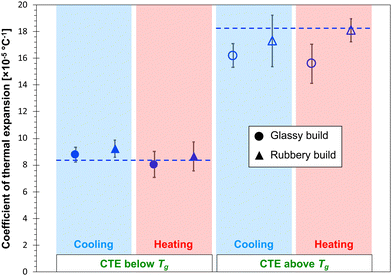
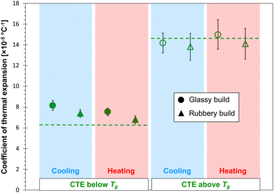
The CTE values of the epoxy and PBZ systems were measured using a thermo-mechanical analyser (TMA Q400, TA Instruments). Four specimens each were cut from panels fabricated as described elsewhere.^4,51 The TMA tests were carried out by placing the specimens on a platform equipped with an expansion probe enclosed in a furnace. A small normal force was applied for the entire duration of the test to maintain contact between the probe and the specimen. Initially, the furnace temperature was equilibrated to 30 °C and the specimen thicknesses were measured. The specimens were heated above T_g at a rate of 5 °C min⁻¹, while the change in thickness was measured as a function of the temperature. The resulting CTE values are provided in Table 1.

Table 1 Measured CTE values of epoxy and PBZ

	Epoxy	PBZ
CTE below Tg (×10^−5 °C^−1)	8.32 ± 0.25	6.36 ± 0.13
CTE above Tg (×10^−5 °C^−1)	18.30 ± 0.19	14.59 ± 3.65

---

Results and discussion

Table 2 shows the predicted glassy and rubbery mass density values for both resin systems and both build types. Experimentally-measured values^4,51 are also included in the table. The data indicates that the predicted mass densities in the glassy state are within 2% of the experimental values, regardless of build temperature. Clearly this indicates that the force field and MD modelling protocols are predicting accurate mass densities, which is an important first step in building accurate MD models of polymer systems. The data in the table also indicates that the difference in the mass densities between glassy and rubbery builds is significantly greater for PBZ than for the epoxy. As described in the ESI,† the uncertainty in predicted values between replicates is likely related to statistical variations in the structure of the crosslinked network.

Table 2 Predicted and experimental values of mass density for epoxy and PBZ resins (g cc⁻¹)

	Glassy build	Rubbery build	Experiment
Epoxy (glassy state)	1.213 ± 0.006	1.210 ± 0.003	1.193^4
Epoxy (rubbery state)	1.168 ± 0.005	1.156 ± 0.004	—
PBZ (glassy state)	1.182 ± 0.002	1.170 ± 0.006	1.182^51
PBZ (rubbery state)	1.133 ± 0.001	1.124 ± 0.004	—

---

Fig. 5 shows the predicted T_g values for the epoxy and PBZ systems for both builds for the cooling and heating cycles. An experimentally-measured value of the T_g for epoxy⁴ from the literature is included, as is a range of measured T_g values of bisphenol-a PBZ from the literature.^64–70 A wide range of T_g values for PBZ exists because of the sensitivity of processing methods on the degree of cure.

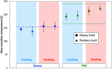Fig. 5 Predicted (data points) and experimental (dashed lines) T_g values for both thermoset systems.

Several important observations can be made from the data in Fig. 5. First, the predicted T_g values, regardless of build and heating/cooling cycle, fall within range of reported experimental T_g values for both systems. Second, the average predicted T_g values for the heating simulations tend to be higher than those from cooling simulations, although this trend is not statistically significant when considering the standard deviation values. Third, there is no statistically significant difference between the T_g values predicted by the glassy and rubbery builds for either resin system. The lack of any statistically significant differences with heating/cooling simulations and build temperatures is likely due to the scatter in predicted properties that is inherent with MD simulations of amorphous systems, which manifests itself in relatively large standard deviations. Thus, any differences in predicted T_g values from different heating/cooling simulations and build temperatures is small enough to be lost in the prediction scatter. It's important to note that if correction factors were used on this data (lowering the T_g by ∼30 °C), the epoxy predictions would be significantly lower than experiment, and the PBZ predictions would be in the lower portion of the experimental range. It's also important to note that, as explained in detail in the ESI,† any effects of simulated cooling rate on the predicted T_g values is too small to be statistically discernible for a range of typical simulated cooling rates.

Fig. 6 and 7 show the predicted CTE values (below and above T_g) for the epoxy and PBZ systems, respectively. The data includes the glassy and rubbery builds, as well as heating and cooling cycles. Experimentally-measured values of CTE for the bis-F epoxy and PBZ systems from Table 1 are included. For both systems, all of the CTE predictions are in reasonable agreement with experiment. There is no consistent, statistically significant difference between the predictions for glassy/rubbery builds and heating/cooling cycles. Similar to the results for T_g, the existence of any such differences is lost in the statistical scatter of the predictions over multiple replicates.

Fig. 6 Predicted (data points) and experimental (dashed lines) CTE values for the epoxy system.

Fig. 7 Predicted (data points) and experimental (dashed lines) CTE values for the PBZ system.

Table 3 provides the predicted Young's modulus for both resin systems at two different temperatures for both glassy and rubbery builds. Experimental values of the PBZ⁵¹ and epoxy from a high-strain rate experiment⁷¹ (as calculated by Odegard et al.⁴) are included for validation. The values of the predicted Young's modulus of PBZ are consistently higher for the glassy build systems, which is expected as the mass densities are consistently higher for the glassy systems (Table 2). For epoxy, the difference between glassy and rubbery builds are not statistically significant, similar to the mass densities (Table 2). Similar trends are observed for predicted bulk (Table S4, ESI†) and shear (Table S5, ESI†) moduli below and above T_g. As described in the ESI,† the uncertainty in predicted values of Young's modulus between replicates is likely related to statistical variations in the structure of the crosslinked network. Values of Poisson's ratio are relatively unaffected by the build temperature (Table S6, ESI†).

Table 3 Predicted and experimental values of Young's modulus for epoxy and PBZ resins

Material	Temperature (°C)	Glassy build (GPa)	Rubbery build (GPa)	Experiment (GPa)
Epoxy	27	3.3 ± 0.8	3.1 ± 0.7	3.3^4,71
	177	2.2 ± 0.7	2.0 ± 0.7	—
PBZ	27	5.6 ± 0.1	4.5 ± 0.3	5.5^51
	200	2.9 ± 0.4	2.5 ± 0.3	—

---

Table 4 provides the predicted yield strength for both resin systems at two different temperatures for both glassy and rubbery builds. Experimental values of the PBZ⁵¹ and epoxy from a high-strain rate experiment⁷¹ (as calculated by Odegard et al.⁴) are included for validation. It's important to note that the discrepancy between predictions and experiment is due to the well-known strain-rate effect, which is significant for yield strength predictions.⁴ The values of the predicted yield strength of PBZ are consistently higher for the glassy build systems, which is expected as the mass densities are consistently higher for the glassy systems (Table 2). For epoxy, the difference between glassy and rubbery builds are not statistically significant, similar to the mass densities (Table 2).

Table 4 Predicted and experimental values of yield strength for epoxy and PBZ resins

Material	Temperature (°C)	Glassy build (MPa)	Rubbery build (MPa)	Experiment (MPa)
Epoxy	27	103 ± 18	91 ± 17	94^4,71
	177	9 ± 3	10 ± 2	—
PBZ	27	132 ± 4	103 ± 9	49^51
	200	88 ± 15	64 ± 5	—

---

Table 5 shows the predicted and experimental^72,73 values of thermal conductivity for both polymer systems. The MD predictions agree well with the experimental measurements in all cases. There is no significant difference in predicted conductivities for the glassy and rubbery builds for both systems. Unlike the mechanical properties discussed above, thermal conductivity is not strongly dependent on mass density, but more closely dependent on the covalently bonded network.^61,63

Table 5 Predicted and experimental values of thermal conductivity for epoxy and PBZ resins

Material	Temperature (°C)	Glassy build (W mC^−1)	Rubbery build (W mC^−1)	Experiment (W mC^−1)
Epoxy	27	0.30 ± 0.02	0.33 ± 0.02	0.2–0.3^72
	177	0.30 ± 0.04	0.30 ± 0.02	—
PBZ	27	0.26 ± 0.03	0.30 ± 0.04	0.23^73
	200	0.28 ± 0.03	0.29 ± 0.02	—

---

Conclusions

The results of the study indicate that the accurate prediction of T_g of thermosetting polymers using all-atom MD simulation depends on the use of appropriate force fields and the building of molecular models with mass densities that are accurate within 2% of experimental values. Cooling rate correction factors, model building within different conformational states, and the choice of heating/cooling simulation runs do not provide statistically significant differences in the accurate prediction of T_g values, given the typical scatter observed in MD predictions of amorphous polymers. Similarly, the accurate prediction of CTE (above and below T_g) is not significantly affected by the MD model build temperature or heat/cooling cycle.

Because the difference in the mass densities between glassy and rubbery builds is significantly greater for PBZ than for epoxy, the predicted Young's modulus and yield strength is significantly affected by build temperature for PBZ, but not for epoxy. Because the thermal conductivity is strongly affected by network morphology and not mass density, the predicted thermal conductivities for the two polymer systems is not affected by the build temperature.

Taking all of these results together, the data indicates that accurate MD predictions of most properties are highly reliant upon accurate predictions of mass density. MD models of amorphous polymers should be built with mass densities that match experiment within 2% for the conformational state of interest (glassy/rubbery). While the conformational state type does not have a statistically significant influence on the prediction of T_g, CTE, and thermal conductivity, it has a significant effect on the prediction of mass density and mechanical properties.

Author contributions

GMO: conceptualization, data curation, formal analysis, funding acquisition, investigation, methodology, project administration, resources, supervision, writing – original draft, writing – review & editing; SUP: conceptualization, data curation, investigation, methodology, visualization, writing – original draft, writing – review & editing; PSG: data curation, investigation, methodology, visualization, writing – original draft, writing – review & editing; PD: conceptualization, data curation, investigation, methodology, visualization, writing – original draft, writing – review & editing; ASK: investigation, formal analysis; SPS: investigation, formal analysis; AR: Investigation, formal analysis; TD: project administration; JAK: project administration; MM: funding acquisition, project administration, writing – review & editing.

Conflicts of interest

There are no conflicts to declare.

Acknowledgements

This research was partially supported by the NASA Space Technology Research Institute (STRI) for Ultra-Strong Composites by Computational Design (US-COMP), grant NNX17AJ32G; and NASA grants 80NSSC19K1246 and 80NSSC21M0104. SUPERIOR, a high-performance computing cluster at Michigan Technological University, was used in obtaining the MD simulation results presented in this publication.

References

1. C. Y. Li and A. Strachan, Polymer, 2011, 52, 2920–2928.
2. C. Y. Li and A. Strachan, J. Polym. Sci., Part B: Polym. Phys., 2015, 53, 103–122.
3. M. S. Radue, V. Varshney, J. W. Baur, A. K. Roy and G. M. Odegard, Macromolecules, 2018, 51, 1830–1840.
4. G. M. Odegard, S. U. Patil, P. P. Deshpande, K. Kanhaiya, J. J. Winetrout, H. Heinz, S. P. Shah and M. Maiaru, Macromolecules, 2021, 54, 9815–9824.
5. S. U. Patil, S. P. Shah, M. Olaya, P. P. Deshpande, M. Maiaru and G. M. Odegard, ACS Appl. Polym. Mater., 2021, 3, 5788–5797.
6. M. S. Radue, B. D. Jensen, S. Gowtham, D. R. Klimek-McDonald, J. A. King and G. M. Odegard, J. Polym. Sci., Part B: Polym. Phys., 2018, 56, 255–264.
7. H. Park, B. Kim, J. Choi and M. Cho, Polymer, 2018, 136, 128–142.
8. V. Varshney, S. Patnaik, A. Roy and B. Farmer, Macromolecules, 2008, 41, 6837–6842.
9. A. Vashisth, C. Ashraf, W. Zhang, C. E. Bakis and A. C. T. van Duin, J. Phys. Chem. A, 2018, 122, 6633–6642.
10. C. E. Estridge, Polymer, 2018, 141, 12–20.
11. T. W. Sirk, K. S. Khare, M. Karim, J. L. Lenhart, J. W. Andzelm, G. B. McKenna and R. Khare, Polymer, 2013, 54, 7048–7057.
12. M. Tsige, C. D. Lorenz and M. J. Stevens, Macromolecules, 2004, 37, 8466–8472.
13. S. V. Kallivokas, A. P. Sgouros and D. N. Theodorou, Soft Matter, 2019, 15, 721–733.
14. J. Buchholz, W. Paul, F. Varnik and K. Binder, J. Chem. Phys., 2002, 117, 7364–7372.
15. J. H. R. Clarke, in The Physics of Glassy Polymers, ed. R. N. Haward and R. J. Young, Chapman & Hall, London, 1997.
16. J. M. Hutchinson, in Physics of Glassy Polymers, ed. R. N. Haward and R. J. Young, Chapman & Hall, London, 1997.
17. G. M. Odegard and A. Bandyopadhyay, J. Polym. Sci., Part B: Polym. Phys., 2011, 49, 1695–1716.
18. K. Vollmayr, W. Kob and K. Binder, J. Chem. Phys., 1996, 105, 4714–4728.
19. J. S. Bermejo and C. M. Ugarte, Macromol. Theory Simul., 2009, 18, 317–327.
20. C. Jang, T. E. Lacy, S. R. Gwaltney, H. Toghiani and C. U. Pittman, Macromolecules, 2012, 45, 4876–4885.
21. P.-H. Lin and R. Khare, Macromolecules, 2009, 42, 4319–4327.
22. N. J. Soni, P.-H. Lin and R. Khare, Polymer, 2012, 53, 1015–1019.
23. C. Y. Li, G. A. Medvedev, E. W. Lee, J. Kim, J. M. Caruthers and A. Strachan, Polymer, 2012, 53, 4222–4230.
24. N. B. Shenogina, M. Tsige, S. S. Patnaik and S. M. Mukhopadhyay, Macromolecules, 2012, 45, 5307–5315.
25. H. B. Fan and M. M. F. Yuen, Polymer, 2007, 48, 2174–2178.
26. A. Bandyopadhyay, P. K. Valavala, T. C. Clancy, K. E. Wise and G. M. Odegard, Polymer, 2011, 52, 2445–2452.
27. N. Nouri and S. Ziaei-Rad, Macromolecules, 2011, 44, 5481–5489.
28. J. Choi, S. Yu, S. Yang and M. Cho, Polymer, 2011, 52, 5197–5203.
29. G. Rossi, I. Giannakopoulos, L. Monticelli, N. K. J. Rostedt, S. R. Puisto, C. Lowe, A. C. Taylor, I. Vattulainen and T. Ala-Nissila, Macromolecules, 2011, 44, 6198–6208.
30. S. R. Yang and J. M. Qu, Polymer, 2012, 53, 4806–4817.
31. A. Izumi, T. Nakao and M. Shibayama, Soft Matter, 2012, 8, 5283–5292.
32. P. V. Komarov, C. Yu-Tsung, C. Shih-Ming, P. G. Khalatur and P. Reineker, Macromolecules, 2007, 40, 8104–8113.
33. F. Jeyranpour, G. Alahyarizadeh and B. Arab, J. Mol. Graphics Modell., 2015, 62, 157–164.
34. Y. Sun, L. Chen, L. Cui, Y. Zhang and X. Du, Comput. Mater. Sci., 2018, 143, 240–247.
35. S. Masoumi, B. Arab and H. Valipour, Polymer, 2015, 70, 351–360.
36. J. Konrad, R. H. Meißner, E. Bitzek and D. Zahn, ACS Polym. Au, 2021, 1, 165–174.
37. M. A. F. Afzal, A. R. Browning, A. Goldberg, M. D. Halls, J. L. Gavartin, T. Morisato, T. F. Hughes, D. J. Giesen and J. E. Goose, ACS Appl. Polym. Mater., 2021, 3, 620–630.
38. K. S. Khare and F. R. Phelan, Macromolecules, 2018, 51, 564–575.
39. J. D. Ferry, Viscoelastic Properties of Polymers, John Wiley & Sons, Inc., New York, 1980.
40. M. L. Williams, R. F. Landel and J. D. Ferry, J. Am. Chem. Soc., 1955, 77, 3701–3707.
41. J. J. Winetrout, K. Kanhaiya, G. Sachdeva, R. Pandey, B. Damirchi, A. van Duin, G. Odegard and H. Heinz, 2021, arXiv:2107.14418.
42. L. Yang, C.-H. Tan, M.-J. Hsieh, J. Wang, Y. Duan, P. Cieplak, J. Caldwell, P. A. Kollman and R. Luo, J. Phys. Chem. B, 2006, 110, 13166–13176.
43. S.-W. Chiu, S. A. Pandit, H. L. Scott and E. Jakobsson, J. Phys. Chem. B, 2009, 113, 2748–2763.
44. S. J. Marrink, H. J. Risselada, S. Yefimov, D. P. Tieleman and A. H. de Vries, J. Phys. Chem. B, 2007, 111, 7812–7824.
45. A. Arkhipov, P. L. Freddolino, K. Imada, K. Namba and K. Schulten, Biophys. J., 2006, 91, 4589–4597.
46. P. T. Underhill and P. S. Doyle, J. Non-Newtonian Fluid Mech., 2004, 122, 3–31.
47. S. Plimpton, J. Comput. Phys., 1995, 117, 1–19.
48. S. U. Patil, M. S. Radue, W. A. Pisani, P. Deshpande, H. Xu, H. Al Mahmud, T. Dumitrică and G. M. Odegard, Comput. Mater. Sci., 2020, 185, 109970.
49. W. A. Pisani, M. S. Radue, S. U. Patil and G. M. Odegard, Composites, Part B, 2021, 211, 108672.
50. P. P. Deshpande, M. S. Radue, P. Gaikwad, S. Bamane, S. U. Patil, W. A. Pisani and G. M. Odegard, Langmuir, 2021, 37, 11526–11534.
51. P. S. Gaikwad, A. S. Krieg, P. P. Deshpande, S. U. Patil, J. A. King, M. Maiaru and G. M. Odegard, ACS Appl. Polym. Mater., 2021, 3, 6407–6415.
52. H. Heinz, T. J. Lin, R. K. Mishra and F. S. Emami, Langmuir, 2013, 29, 1754–1765.
53. S. Nose, Mol. Phys., 1984, 52, 255–268.
54. S. Nosé, J. Chem. Phys., 1984, 81, 511–519.
55. W. G. Hoover, Phys. Rev. A: At., Mol., Opt. Phys., 1985, 31, 1695–1697.
56. J. R. Gissinger, B. D. Jensen and K. E. Wise, Polymer, 2017, 128, 211–217.
57. J. L. Tack and D. M. Ford, J. Mol. Graphics Modell., 2008, 26, 1269–1275.
58. H. Al Mahmud, M. S. Radue, S. Chinkanjanarot, W. A. Pisani, S. Gowtham and G. M. Odegard, Composites, Part B, 2019, 172, 628–635.
59. L. E. Malvern, Introduction to the Mechanics of a Continuous Medium, Prentice-Hall, Inc., Upper Saddle River, NJ, 1969.
60. G. M. Odegard, B. D. Jensen, S. Gowtham, J. Y. Wu, J. Y. He and Z. L. Zhang, Chem. Phys. Lett., 2014, 591, 175–178.
61. X. Wan, B. Demir, M. An, T. R. Walsh and N. Yang, Int. J. Heat Mass Transfer, 2021, 180, 121821.
62. S. Chinkanjanarot, M. S. Radue, S. Gowtham, J. M. Tomasi, D. R. Klimek-McDonald, J. A. King and G. M. Odegard, J. Appl. Polym. Sci., 2018, 135, 46371.
63. V. Varshney, S. S. Patnaik, A. K. Roy and B. L. Farmer, Polymer, 2009, 50, 3378–3385.
64. H. Ishida and H. Y. Low, Macromolecules, 1997, 30, 1099–1106.
65. E. M. Nour-Eddine, Q. Yuan and F. Huang, J. Appl. Polym. Sci., 2012, 125, 1773–1781.
66. S. Rimdusit, P. Kunopast and I. Dueramae, Polym. Eng. Sci., 2011, 51, 1797–1807.
67. S. Rimdusit, W. Bangsen and P. Kasemsiri, J. Appl. Polym. Sci., 2011, 121, 3669–3678.
68. Y.-C. Su, S.-W. Kuo, D.-R. Yei, H. Xu and F.-C. Chang, Polymer, 2003, 44, 2187–2191.
69. J.-M. Huang and S.-J. Yang, Polymer, 2005, 46, 8068–8078.
70. C. Jubsilp, T. Takeichi and S. Rimdusit, Polym. Degrad. Stab., 2011, 96, 1047–1053.
71. A. Gilat, K. Goldberg Robert and D. Roberts Gary, J. Aerosp. Eng., 2007, 20, 75–89.
72. S. Ganguli, A. K. Roy and D. P. Anderson, Carbon, 2008, 46, 806–817.
73. Y. Wang, W. Wu, D. Drummer, C. Liu, W. Shen, F. Tomiak, K. Schneider, X. Liu and Q. Chen, Mater. Des., 2020, 191, 108698.

---

Footnote

† Electronic supplementary information (ESI) available. See DOI: https://doi.org/10.1039/d2sm00851c

---