
 Open Access Article
 This Open Access Article is licensed under a
 Creative Commons Attribution 3.0 Unported Licence
Gradient copolymers versus block copolymers: self-assembly in solution and surface adsorption
Jonathan G.
Coldstream
 a,
Philip J.
Camp
*a,
Daniel J.
Phillips
b and
Peter J.
Dowding
b
a,
Philip J.
Camp
*a,
Daniel J.
Phillips
b and
Peter J.
Dowding
b
aSchool of Chemistry, University of Edinburgh, David Brewster Road, Edinburgh EH9 3FJ, Scotland, UK. E-mail: philip.camp@ed.ac.uk; Tel: +44 131 650 4763
bInfineum UK Ltd., P.O. Box 1, Milton Hill, Abingdon OX13 6BB, England, UK
First published on 2nd August 2022
Abstract
The structures of amphiphilic block and gradient copolymers in solution and adsorbed onto surfaces are surveyed using molecular-dynamics simulations. A bead-spring model is used to identify the general effects of the different architectures: block and gradient copolymers have equal numbers of solvophilic and solvophobic beads, and the gradient copolymer is represented by a linear concentration profile along the chain. Each type of isolated copolymer forms a structure with a globular head of solvophobic beads, and a coil-like tail of solvophilic beads. The radius of gyration of a gradient copolymer is found to be much more sensitive to temperature than that of a block copolymer due to an unravelling mechanism. At finite concentrations, both gradient and block copolymers self-assemble into micelles, with the gradient copolymers again showing a larger temperature dependence. The micelles are characterised using simulated scattering profiles, which compare favourably to existing experimental data. The adsorption of copolymers onto structureless surfaces is modelled with an attractive potential that is selective for the solvophobic beads, and the surface structures are characterised using the average height of the molecules, and the proportion of beads adsorbed. Both types of copolymer form adsorbed films with persistent micelle-like structures, but the gradient copolymers show a stronger dependence on the strength of the surface interactions and the temperature. Coarse-grained, bead-spring models allow a rapid survey and comparison of the block and gradient architectures, and the results set the scene for future work with atomistic simulations. A superficial but favourable comparison is made between the results from the bead-spring models, and atomistic simulations of a butyl prop-2-enoate/prop-2-enoic acid (butyl acrylate/acrylic acid) copolymer in n-dodecane at room temperature.
1 Introduction
Amphiphilic copolymers in selective solvents exhibit structures that depend strongly on the sequence of monomers in the polymer chain.1–7 The dependence of structure on architecture allows fine tuning of polymer properties for specific applications. Block copolymers consist of two segments with an abrupt change in composition from one type of monomer to another. These have been extensively studied in solution, and shown to form a wide range of self-assembled structures.8–10 In contrast to a block copolymer, gradient copolymers are described by a smooth transition from one type of monomer to another along the length of the chain. The gradual change from solvophilic to solvophobic units along the chain gives the copolymers interesting properties, such as thermal responsiveness,11 which make them suited to a wide range of applications. These include stabilisers for immiscible polymer blends,12 damping materials,13 and in pharmaceutical science as drug-delivery media.14–17Another potential application of copolymers is as lubricant additives. Lubricants consist of a package of various additives in a base oil. Polymeric molecules are often included as friction modifiers,18–20 and as viscosity modifiers.21 Gradient copolymers have been identified as being potentially useful as viscosity modifiers. The addition of gradient copolymers to base oils has been shown experimentally to reduce the temperature dependence of viscosity, when compared to the unmodified base oil.22 This is desirable as a large temperature dependence can lead to inconsistent performance of a lubricant over the wide range of temperatures that engines experience.
Block copolymers have been shown to have rich self-assembly behaviour, and can form many distinct structures including micelles, cylindrical micelles, and vesicles, among others.8,23,24 Gradient copolymers have also been shown experimentally to form micelles in solution depending on temperature,25,26 pH,27 and solvent quality.28 Self-assembly of gradient copolymers to form micelles has been studied computationally using lattice Monte Carlo techniques,29,30 and off-lattice, bead-spring models.31 The formation of micelles was shown to depend on both the strength of solvent selectivity, and the polymer architecture. Overall, though, the body of literature on modelling gradient copolymers is still sparse, and one of the aims of the current work is to emphasise some of the key differences between block and gradient copolymers.
In this work, molecular dynamics simulations of a simple bead-spring model are used to survey the structures formed by gradient and block copolymers both in solution, and at the solution–solid interface. Beginning with isolated copolymers, the dependence of the molecular conformation on architecture and temperature is determined; some comparisons with statistical (random) copolymers are also made. Solutions at finite concentration are then studied, and simulated scattering data are presented and compared to available data from neutron-scattering experiments. Simulations of gradient and block copolymers on selectively adsorbing surfaces are presented to show the types of structures formed at different temperatures and surface-interaction strengths. The results from these coarse-grained, bead-spring models provide a template for analysing all-atom simulations in the future. This is illustrated with preliminary simulations of a butyl prop-2-enoate/prop-2-enoic acid (butyl acrylate/acrylic acid) copolymer in n-dodecane at room temperature, which show the fidelity of the coarse-grained model.
The rest of the article is organised as follows. The simulation models and methods are detailed in Section 2. Section 3 reports the results from coarse-grained simulations of isolated copolymers in solution (3.1), many copolymers in solution (3.2), isolated adsorbed copolymers (3.3), and many adsorbed copolymers (3.4), and from atomistic simulations of isolated copolymers in solution (3.5). Section 4 concludes the article.
2 Simulation models and methods
2.1 Polymer sequences
This work is focused on two types of copolymer. The first type is a block copolymer, consisting of two different, but equally long blocks with uniform chemical composition; one block is composed of N1 solvophilic monomers, and the other of N2 = N1 solvophobic monomers. The total number of monomer units is N = N1 + N2, and they are labelled sequentially from i = 0 to i = N − 1. The second type is a gradient copolymer. Instead of a sharp interface between two blocks, there is a smooth transition from one type of monomer to another. To model these sequences a straight gradient model is used. This was chosen as a first approximation of a gradient copolymer to try and maximise any differences that might occur between the block and gradient architectures. In what follows, a few results will also be shown for statistical copolymers, where the composition varies randomly along the chain. Each monomer at a fractional position x = i/(N − 1) along the chain has a certain probability p1(x) to be of type 1. Continuous versions of the probability densities for block, gradient, and statistical (random) copolymers are plotted in Fig. 1. Monomer sequences were sampled from these distributions. Note that for the gradient copolymer, since p1(0) = 1 and p1(1) = 0, and the interpolation is linear, there are equal numbers of type 1 and type 2 beads. | ||
| Fig. 1 (Top) Chemical compositions of block, gradient, and statistical copolymers as functions of the fractional positions x along the chains. p1(x) is the probability density of solvophilic (type 1) monomers. (Bottom) Example distributions are shown for (a) block, (b) gradient, and (c) statistical copolymers. | ||
2.2 Coarse-grained model and molecular-dynamics simulations
Bead-spring models have been widely used to study the universal properties of polymers.32–35 The idea behind the model stems from the loss of directional correlation between segments above a certain characteristic distance along the polymer known as the Kuhn length.36 The result of this is that many structural properties of polymers above this length scale are independent of the precise chemical detail of the polymer, and often follow universal scaling laws.37–40 For homopolymers in solution, this results in the characteristic Flory exponent, with the radius of gyration (Rg) of the polymer scaling as Rg ∼ Nν, with ν = 0.588 in good solvent, ν = 1/2 for a random walk polymer in a θ-solvent, and ν = 1/3 in bad solvent. Similar scaling laws have been found for homopolymers37,41 and star polymers42 adsorbing to surfaces.The use of a coarse-grained model also helps to reduce the high computational cost of simulating polymers using an all-atom model. The sizes of typical polymer molecules require many solvent molecules to be included in explicit-solvent simulations. Much of the computational time is then spent calculating the structure and dynamics of the solvent, rather than those of the polymer. As a result, coarse-grained polymer models, using an implicit solvent, are often used as the solution to this problem. The bead-spring model used here consists of N beads of mass m with contiguous beads connected by a spring potential. If N is small, then the composition gradient in the gradient copolymer is large, and the molecule resembles a block copolymer. If N is large, then the computational cost of simulating many copolymers is prohibitively high. Most calculations were carried out with N = 256, so that the difference between p1 on neighbouring beads in the gradient copolymer was small, but some spot checks were made with N varying from 16 to 512. Each bead models either a solvophilic or a solvophobic segment of the chain. Here the bonds are modelled by a finitely extensible nonlinear elastic (FENE) potential of the form
 | (1) |
 | (2) |
 | (3) |
 | (4) |
 | (5) |
 | (6) |
 .
.
All simulations were performed in the NVT ensemble using the Nosé–Hoover thermostat with a timestep of δt = 0.002τ, where  . The dimensionless temperature is defined as T* = kBT/ε. The values of the FENE constants were set at R0 = 1.5σ and k = 30ε/σ2, which have been used in previous studies using a similar model.43 Simulation protocols for specific systems will be described in the relevant parts of Section 3. The LAMMPS package was used throughout.44–46
2.3 Atomistic model and molecular-dynamics simulations
All-atom molecular dynamics simulations of block and gradient copolymers were performed using the LAMMPS package.44–46 Each copolymer consisted of equal numbers of butyl prop-2-enoate and prop-2-enoic acid monomer units, and a single molecule was solvated in n-dodecane. Interatomic potentials were described using the OPLS-AA force field,47,48 with the LJ interactions cut off at 12 Å. Coulombic interactions were calculated using a particle–particle particle-mesh implementation of the Ewald summation. Simulations were run from initial configurations built using Packmol.49 Each system was equilibrated in a cubic box, with periodic boundary conditions applied in all three dimensions, and a time step of δt = 1 fs. A short run of 0.5 ns in the NVT ensemble was followed by at least 10 ns in the NPT ensemble with T = 298 K and P = 1 atm.3 Results
3.1 Coarse-grained models: a single copolymer in solution
The effects of monomer distribution on the conformation of a single copolymer are presented in this section. Simulations were performed in a cubic box with side L = 50σ, and with periodic boundary conditions applied in all three dimensions. L was chosen to be large enough to avoid the molecule interacting with its own periodic image. Systems were equilibrated for 5 × 10⁶ δt before a production run of at least 2 × 10⁷ δt. Simulations of the gradient and statistical copolymers were repeated eight times with different monomer sequences drawn from the appropriate type-1 bead distribution, and the results were averaged. Some snapshots of isolated block, gradient, and statistical copolymers are shown in Fig. 2. At both ends of the temperature scale considered here, the block copolymer forms a structure containing a spherical head of solvophobic beads, which minimises the bead–solution interfacial area, and a long tail of solvophilic beads, which is swollen in solution. Ostensibly, the gradient copolymer shows the same kind of structure, but the segregation of the solvophilic and solvophobic beads between the tail and the head is less pronounced. Moreover, at high temperature, there are solvophobic beads in the tail part of the structure. The statistical copolymer switches from a low-temperature globular form, to a high-temperature coil-like form, without any distinct head or tail motifs. | ||
| Fig. 2 Snapshots of isolated block, gradient, and statistical copolymers in solution: (a), (b), and (c) show block, gradient and statistical copolymers, respectively, at T* = 1.0; (d), (e), and (f) are the equivalent snapshots for T* = 2.0. Solvophobic beads are shown in orange, and solvophilic beads are shown in blue. | ||
The effects of increasing temperature on molecular conformation were quantified using the radius of gyration Rg defined by
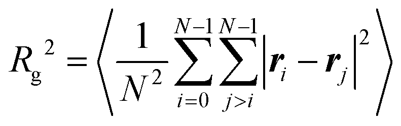 | (7) |
 | ||
| Fig. 3 The radius of gyration of (a) all beads, and (b) each type of bead, in the temperature range 1.0 ≤ T* ≤ 2.0, for block, gradient, and statistical copolymers. In (b) the dashed lines are for the solvophilic beads, and the dotted lines are for the solvophobic beads. | ||
The scaling law Rg ∼ Nν was determined for block and gradient copolymers at T* = 1.0, with N ranging from 16 to 512. The fitted Flory exponents were ν = 0.60 ± 0.04 for block copolymers, and ν = 0.50 ± 0.02 for gradient copolymers. This shows that the radius of gyration of the block copolymer is dictated by the solvophilic block, and so it scales according to the prediction for good-solvent conditions. For the gradient copolymer, the scaling is somewhere between the bad-solvent and good-solvent cases, as has been observed in experiments.11 The similarity with the random-walk exponent is probably coincidental.
To summarise, the radii of gyration of gradient and statistical copolymers depend sensitively on temperature, while displaying very different structures. The structure of the gradient copolymer looks much like that of the block copolymer, while the statistical copolymer forms an isotropic globular structure. Hereafter, the focus will be on the differences between block and gradient copolymers.
3.2 Coarse-grained models: many copolymers in solution
The self-assembly of copolymers to form micelles is an important phenomenon in soft-matter science. To study this, 50 copolymer chains of a given type were placed randomly into a cubic box with side L = 500σ, which was then shrunk in steps to L = 150σ over a period of 1 × 10⁶ δt. The final concentration was ρ* = Nσ3/V = 0.00379, which corresponds to a volume fraction of about 0.2%. The system was then equilibrated for 5 × 10⁷ δt, before a production run of 1 × 10⁷ δt.Simulation snapshots of block copolymers are shown in Fig. 4(a) and (c). The molecules aggregate into micelles consisting of a densely packed core of solvophobic beads surrounded by a corona of swollen solvophilic arms. The driving force for aggregation is the interaction energy between beads in bad solvent, and as the aggregation number increases, so does the number of good-solvent arms around the core; further aggregation is prevented by the entropic repulsion between those arms.
 | ||
| Fig. 4 Snapshots of many block and gradient copolymers in solution: (a) and (b) show structures formed by block and gradient copolymers, respectively, at T* = 1.0; (c) and (d) are the equivalent snapshots for T* = 2.0. Solvophobic beads are shown in orange, and solvophilic beads are shown in blue. | ||
Important experimental techniques for characterising micellar structures include small-angle neutron and X-ray scattering. In an isotropic system, the dependence of the scattering intensity I(q) on the magnitude of the wave vector q (and scattering angle) is given by
 | (8) |
Fig. 5 shows the total scattering [in (a)], and the partial functions [in (c) and (e)], for block copolymers at 1.0 ≤ T* ≤ 2.0. As for the radius of gyration, the partial functions are computed by restricting the sums in eqn (8) to beads of a given type. The first thing to note is that the scattering profiles are qualitatively similar at different temperatures, implying that an increase in T* has a small effect on the structure of the micelles. Given that the radius of gyration of an isolated block copolymer changes little with increasing temperature (Fig. 3), one might expect the size of a micelle to also be quite insensitive to temperature. At low micelle concentrations, the low-q behaviour of I(q) is largely controlled by the micelle radius of gyration, according to the Guinier law I(q) ≈ 1 − q2Rg2/3, and so its insensitivity to temperature is consistent with expectations. The main difference is in the partial scattering function for the solvophobic (attractive) particles at high wave vectors 1 < qσ < 10, which shows a less-deep minimum with increasing temperature. This shows that the solvophobic core structure changes, while the solvophilic arms are hardly affected by temperature.
 | ||
| Fig. 5 Scattering intensities of a block copolymer solution [(a), (c), (e)] and a gradient copolymer solution [(b), (d), (f)] with ρ* = 0.00379 and at various temperatures. (a) and (b) show the total scattering intensity, (c) and (d) show the partial scattering intensity for the solvophilic (repulsive) beads, and (e) and (f) show the partial scattering intensity for the solvophobic (attractive) beads. The yellow lines in (a) and (b) are fits of eqn (9) to the data for T* = 1.0 in the range qσ ≤ 0.2. The dashed line in (c) has the form I(q) ∝ q−3/2. | ||
Fig. 5(c) shows the scattering intensity for the solvophilic (repulsive) beads. The scattering intensity at intermediate values 0.5 < qσ < 2.0 decays approximately according to the scaling law q−D, where D ≃ 1.5 in this case. Scattering intensities of polymers at intermediate values of q often show scaling behaviour which characterises the mass-fractal dimension, or how the size of the polymer scales with mass. This is the approach of the Porod plot.50 The value of D is related to the Flory exponent ν by the relation D = 1/ν.51 Here ν ≈ 2/3 which implies a swollen chain in good solvent, but with a larger value of ν than an isolated homopolymer in good solvent (ν = 0.588). Fig. 5(e) shows the scattering intensity for the solvophobic (attractive) beads, and the small peak at qσ ≃ 0.6–0.8 signals that the core is around 8–10 particles across, in correspondence with the snapshots.
Fig. 4(b) and (d) show simulation snapshots of the gradient copolymer micelles at T* = 1.0 and T* = 2.0, respectively. The gradient copolymers form distinct micelles at low temperature. Fig. 5 shows the total scattering [in (b)], and partial functions [in (d) and (f)], for gradient copolymers at 1.0 ≤ T* ≤ 2.0. As temperature increases, I(q) at low q decays slightly more rapidly, and according to the Guinier law, this suggests that the radius of gyration of a micelle increases slightly with increasing temperature. This is broadly consistent with the individual molecules expanding, as shown in Fig. 3. Unlike the block copolymer, the segregation of solvophobic and solvophilic beads at the interface between the core and corona is not very strong. The presence of attractive beads in the micelle arms causes them to form loops attached to the micelle core, similar to the ‘reel in’ effect observed with the isolated copolymers in solution. The snapshot at T* = 2.0 shows that, while micelles still form at higher temperatures, there are also individual copolymers in solution which are in equilibrium with the micelle. This is due to the thermal energy becoming more significant when compared to ε, and the interaction energy is then less significant when compared to the loss of entropy the molecule experiences when joining the micelle. The partial scattering profile for the repulsive beads does not show the power-law scaling behaviour seen with the block copolymers, due to the mixing of repulsive and attractive beads.
An obvious fitting function for I(q) is the form factor of a core–shell model, given by
| I(q) = 9[yf(qR2) + (1 − y) f(qR1)]2 | (9) |
![[thin space (1/6-em)]](https://www.rsc.org/images/entities/char_2009.gif) x − xcosx)/x3, and 0 ≤ y ≤ 1 reflects the volumes, concentrations, and scattering contrasts of the core and the shell. Examples of fitting this equation to the simulation data at T* = 1.0 are shown in Fig. 5(a) and (b). The fits were restricted to the range qσ ≤ 0.2, but the accuracy is not very good. For the block copolymer, y = 0.69 ± 0.01, R1 = (10 ± 1)σ, and R2 = (85 ± 1)σ, confirming that there is a compact core of solvophobic beads, and a dilute corona of solvophilic beads with a thickness of less than half a polymer chain. For the gradient copolymer, y = 0.634 ± 0.007, R1 = (12.9 ± 0.6)σ, and R2 = (78.2 ± 0.6)σ, indicating that the core is slightly less compact, and the corona is slightly less thick, due to the mixing of solvophobic and solvophilic beads. The fits are less good at higher temperature, because the micelle structures are less well defined.
x − xcosx)/x3, and 0 ≤ y ≤ 1 reflects the volumes, concentrations, and scattering contrasts of the core and the shell. Examples of fitting this equation to the simulation data at T* = 1.0 are shown in Fig. 5(a) and (b). The fits were restricted to the range qσ ≤ 0.2, but the accuracy is not very good. For the block copolymer, y = 0.69 ± 0.01, R1 = (10 ± 1)σ, and R2 = (85 ± 1)σ, confirming that there is a compact core of solvophobic beads, and a dilute corona of solvophilic beads with a thickness of less than half a polymer chain. For the gradient copolymer, y = 0.634 ± 0.007, R1 = (12.9 ± 0.6)σ, and R2 = (78.2 ± 0.6)σ, indicating that the core is slightly less compact, and the corona is slightly less thick, due to the mixing of solvophobic and solvophilic beads. The fits are less good at higher temperature, because the micelle structures are less well defined.
Considering together the snapshots in Fig. 4 and the scattering intensities in Fig. 5, it is clear that the micelles formed by block copolymers show greater thermal stability than those formed by gradient copolymers. By visual inspection, Fig. 4(a) and (c) for the block copolymers at low and high temperature each show 6 or 7 micelle cores, indicating an aggregation number of 7 or 8 molecules. For the gradient copolymers, while there are 5 distinct micelle cores at low temperature [Fig. 4(b)], the structures at high temperature are much less well defined. It should be noted, however, that the present study is limited to self-assembled structures with aggregation numbers of 50 or fewer molecules. The fact that several distinct clusters are visible in Fig. 4 suggests that the system sizes are just about large enough for the present purposes. But it cannot be ruled out that at higher concentrations, self-assembled structures (such as cylindrical micelles and vesicles) containing more than 50 of these molecules could form.
Okabe et al. used small-angle neutron scattering (SANS) to characterise the structures of block and gradient copolymer micelles.25,26 Of particular note is Fig. 8 of ref. 25, which shows a direct comparison of the SANS profiles for 0.3 wt% solutions of block and gradient copolymers of 2-ethoxyethyl vinyl ether and 2-methoxyethyl vinyl ether in water. In each case, and at 25 °C, the scattering looks very similar to that shown in Fig. 5(a) and (b), and there is a peak at q ≃ 0.03 Å−1. The simulated profiles show peaks at qσ ≃ 0.1, which suggests a mapping between the coarse-grained models and the real copolymers with the choice σ = 3.3 Å, which is physically reasonable. From the scattering at low wave vectors, and at low temperature (15 °C), Okabe et al. inferred a segment length of around 5 Å, and a radius of gyration of about 70 Å. This means that Rg/σ ≃ 14, which is close to the values at the upper end of the temperature scale considered here [Fig. 3(a)], even without trying to map the lengths of the real and simulated chains onto one another.
3.3 Coarse-grained models: adsorption of a single copolymer
The adsorption of polymers onto surfaces is important for a wide range of technologies, such as coatings, colloid stabilisation, friction modification, and sensors. The interplay between self-assembly and adsorption of such molecules on surfaces can be examined using techniques such as atomic force microscopy, and complemented with simulations.41,42,52,53 The adsorption of isolated block and gradient copolymers is considered here first. The beads in bad solvent are taken to experience an attractive potential with the surface, while the beads in good solvent experience a short range repulsion. Simulations were performed in cubic boxes with side L = 100σ, and with periodic boundary conditions applied in the x and y directions. The z dimension is bounded by two parallel, structureless, and planar surfaces, the effects of which are modelled by eqn (5) and (6). The separation between the surfaces in the z direction is large enough so that a copolymer cannot interact with more than one surface at a time. Systems were equilibrated for at least 5 × 10⁶ δt, before a production run of 2 × 10⁷ δt was performed. Simulations for gradient copolymers were repeated eight times with different monomer sequences drawn from the type-1 probability distribution.Some simulation snapshots are shown in Fig. 6. Fig. 6(a) and (c) show that the block copolymer always adsorbs via its globular, solvophobic head. With weaker surface interactions and at lower temperature ( and T* = 1.0), the head is quite compact, while with stronger surface interactions and at higher temperature (
 and T* = 1.5), the head flattens out. The behaviour of the gradient copolymer changes qualitatively as
  and T* are increased. With the smaller values of these parameters, the conformation is not very different from that of the block copolymer, while with the larger values, the adsorption of the copolymer is more complete, with isolated clusters of solvophobic beads pinning the chain onto the surface, and the formation of loops and a tail.
 | ||
Fig. 6 Snapshots of isolated block and gradient copolymers adsorbed on a surface: (a) a block copolymer with  and T* = 1.0; (b) a gradient copolymer with and T* = 1.0; (b) a gradient copolymer with  and T* = 1.0; (c) a block copolymer with and T* = 1.0; (c) a block copolymer with  and T* = 1.5; (d) a gradient copolymer with and T* = 1.5; (d) a gradient copolymer with  and T* = 1.5. Solvophobic beads are shown in orange, and solvophilic beads are shown in blue. and T* = 1.5. Solvophobic beads are shown in orange, and solvophilic beads are shown in blue. | ||
Fig. 7 shows the probability density distribution p(z) that a bead is at a distance z from the surface. Fig. 7(a) and (b) show the distributions for block and gradient copolymers, respectively, with  and 1.0 ≤ T* ≤ 2.0, and Fig. 7(c) and (d) are the same but with
  and T* = 1.0. The distributions are normalised so that
  . In all cases, there is a peak in the distribution at z ≃ 0.86σ, which corresponds to the minimum in the attractive surface potential [eqn (5)]. Further peaks in the distribution correspond to roughly what would be expected for close packed spheres, with the second peak occurring at z ≃ 1.7σ. These spatial correlations are localised within the compact solvophobic end of the copolymer adsorbing to the surface.
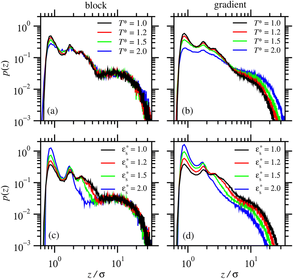 | ||
Fig. 7 Probability density distribution of a bead being a perpendicular distance z from the surface. (a) and (b) show isolated block and gradient copolymers, respectively, with  and 1.0 ≤ T* ≤ 2.0. (c) and (d) show block and gradient copolymers, respectively, with and 1.0 ≤ T* ≤ 2.0. (c) and (d) show block and gradient copolymers, respectively, with  and T* = 1.0. and T* = 1.0. | ||
Fig. 8(a) and (c) show the average bead heights of the block copolymer chains from the surface with  and 1.0 ≤ T* ≤ 2.0, both the overall average, and the average for each bead type. These averages are defined with relations of the form
  . There is a decrease in height of the attractive beads with increasing strength of surface interaction, which corresponds to the flattening of the solvophobic head to the surface. There is little effect on the average height of the solvophilic beads, as they only interact through a short range repulsive interaction. Therefore, an adsorbed block copolymer is effectively a solvophilic homopolymer grafted to the surface, and its conformation is insensitive to temperature.
 | ||
Fig. 8 (a) and (b): the average height of the beads of an isolated block copolymer (a) and an isolated gradient copolymer (b) with  and 1.0 ≤ T* ≤ 2.0. (c) and (d): the average heights of the solvophilic beads (dashed lines) and solvophobic beads (dotted lines) for isolated block and gradient copolymers under the same conditions. (e) and (f): the average fraction of adsorbed beads for isolated block and gradient copolymers under the same conditions. and 1.0 ≤ T* ≤ 2.0. (c) and (d): the average heights of the solvophilic beads (dashed lines) and solvophobic beads (dotted lines) for isolated block and gradient copolymers under the same conditions. (e) and (f): the average fraction of adsorbed beads for isolated block and gradient copolymers under the same conditions. | ||
The extent of the adsorption is measured with the average fraction of beads, fads, that are within the range z ≤ 1.3σ of the surface; this cut off was chosen on the basis that all of the bead density profiles have a first local minimum at approximately this value. Fig. 8(e) shows fads for a block copolymer with  and 1.0 ≤ T* ≤ 2.0. There is a small decrease in fads as temperature increases with each value of
  . The increase in fads with increasing
  again corresponds to the flattening of the solvophobic head to the surface. This is analogous to a wetting process, as the bead–surface attraction becomes much stronger than the bead–bead attraction.
As noted above, while gradient copolymers form qualitatively similar structures when compared to block copolymers adsorbed to surfaces at low  and T*, they react very differently to increases in those parameters. Fig. 7(b) shows the height distributions for gradient copolymers with
  and 1.0 ≤ T* ≤ 2.0. With a fixed value of
  , the primary peak height decreases as temperature increases; also, p(z) dies off at longer distances, corresponding to increased desorption of the polymer tail. The total average height of the gradient copolymer beads is shown in Fig. 8(b), and the individual average heights by bead type are shown in Fig. 8(d), over the ranges
  and 1.0 ≤ T* ≤ 2.0. The average height of the copolymer increases with increasing temperature for both types of bead, and at all values of
  , corresponding to gradual desorption. In contrast to the block copolymer, the heights of the repulsive beads also show a strong temperature dependence; the attractive beads pin down parts of the tail of the copolymer to the surface, and reduce the average height of the repulsive beads. Fig. 8(f) shows the average fraction of adsorbed beads for a gradient copolymer with 1.0 ≤ T* ≤ 2.0 and
  . The fraction of adsorbed beads decreases dramatically with temperature at all values of
  . There are two mechanisms behind this. Firstly, the unravelling of the solvophobic head of the copolymer produces a smaller head and a longer tail, much like the isolated copolymers in solution. Secondly, the solvophilic end of the copolymer can also adsorb onto the surface, pinned by small groups of solvophobic beads. Moving along the chain of the gradient copolymer, the local concentration of beads attracted to the surface decreases. At a certain point the energy of adsorption is no longer high enough to overcome the loss of entropy the chain experiences when it is close to the surface. As the temperature increases, the threshold concentration of repulsive beads, where tail adsorption is no longer favourable, decreases. This has the effect of creating loops in the adsorbed copolymer, as well as increasing the length of the desorbed tail of the copolymer. This mechanism for tail adsorption has a dramatic effect on the average height of the beads. This behaviour is much more complex than that of the block copolymer, and is difficult to capture in a simple theoretical analysis.
Fig. 8 does not show points for the gradient copolymer with  and T* = 2.0, as it desorbs under these conditions. The solvophobic end of the molecule is not solvophobic enough to lead to adsorption, as compared to the block copolymer.
3.4 Coarse-grained models: adsorption of many copolymers
Simulations were performed with 50 chains of N = 256 beads on a square surface of side lengths Lx = Ly = 100σ, 125σ, 150σ, 300σ, and 500σ, giving surface bead concentrations in the range , and area fractions
  . Individual chains were placed close to a surface in a box with Lx = Ly = 500σ and Lz = 100σ. The z dimension of the box was chosen to be large enough so that the copolymers remained adsorbed on that one surface. The x and y dimensions were then shrunk to the desired size over a period of 1 × 10⁶ δt, and equilibrated for 5 × 10⁶ δt, before a production run of 1 × 10⁷ δt was performed.
Fig. 9 shows structures of block and gradient copolymers adsorbed on a surface with Lx = Ly = 125σ. With  and T* = 1.0, both the block and the gradient copolymers form distinct surface-adsorbed micelles. This closely mirrors the formation of micelles in solution, as described in Section 3.2. With
  and T* = 2, the two architectures show very different behaviour. The block copolymers form fewer, larger micelles, in order to optimise the interactions between beads, and between beads and the surface; as the micelles flatten to the surface, they combine with their neighbours and form fewer, flatter aggregates until the surface is covered. The gradient copolymers no longer form distinct surface-adsorbed micelles, and instead, there is a loose network of molecules flat on the surface. This is a drastic difference between the two architectures.
 | ||
Fig. 9 Snapshots of block and gradient copolymers adsorbed on a surface with Lx = Ly = 125σ: (a) block copolymers, and (b) gradient copolymers, with  and T* = 1.0; (c) block copolymers, and (d) gradient copolymers, with and T* = 1.0; (c) block copolymers, and (d) gradient copolymers, with  and T* = 2.0. Solvophobic beads are shown in orange, and solvophilic beads are shown in blue. and T* = 2.0. Solvophobic beads are shown in orange, and solvophilic beads are shown in blue. | ||
As with the study of single-copolymer adsorption, the film structure can be characterised with the fraction of adsorbed beads fads, and the average bead height 〈z〉. fads is plotted for block copolymers in Fig. 10(a)–(c), adsorbed on surfaces with  ,
,  , and
, and 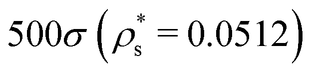 , and with
  and 1.0 ≤ T* ≤ 2.0. In general, fads increases with increasing
  , but there is a big jump between
  . This is due to the bead–surface interaction dominating the bead–bead interaction, and the solvophobic core flattening on the surface. A more interesting effect is that, with
  , increasing the temperature leads to a slight decrease in fads, while with
  , there is a slight increase. One explanation for this is that with high
  , increasing temperature only diminishes the structuring within the solvophobic core, and beads released from the core are strongly attracted to the surface. With low
  , increasing temperature leads to both desorption and disordering of the solvophobic core.
 | ||
Fig. 10 (a)–(c) the fraction of adsorbed beads, and (d)–(f) the average heights of the beads, for block copolymers adsorbed on a surface with Lx = Ly = 100σ, 150σ, and 500σ, and with  and 1.0 ≤ T* ≤ 2.0. and 1.0 ≤ T* ≤ 2.0. | ||
These effects are mirrored in the behaviour of 〈z〉, shown in Fig. 10(d)–(f) for the same block-copolymer systems. With  , increasing the temperature leads to a larger average height as beads desorb. With
  , the opposite trend is observed because of beads being released from the solvophobic core, and adsorbed onto the surface.
The effect of increasing the surface concentration is to increase the average height of the copolymer beads, as the aggregation number of the micelles increases, and the solvophobic core grows laterally and vertically. This is shown for block copolymers in Fig. 11(a)–(c), where the results are plotted as functions of  for
for  , and 1.0 ≤ T* ≤ 2.0. The dependence on the temperature is rather weak, while increasing
  leads to a flattening of the copolymer onto the surface.
 | ||
Fig. 11 The average height of the beads as a function of surface concentration for (a)–(c) block copolymers, and (d)–(f) gradient copolymers. Results are shown for systems with 1.0 ≤ T* ≤ 2.0: (a) and (d)  ; (b) and (e) ; (b) and (e)  ; (c) and (f) ; (c) and (f)  . . | ||
The characterisation of self-assembled and adsorbed gradient copolymers reflects the very different behaviour illustrated in Fig. 9. Fig. 12(a)–(c) show the fraction of adsorbed beads as a function of temperature, for systems adsorbed on surfaces with Lx = Ly = 100σ, 150σ, and 500σ, and with  . In all cases, fads decreases with increasing temperature. Similar to the isolated copolymer on a surface, as T* increases, the arms desorb closer to the solvophobic cores of the micelles due to the decreasing concentration of attractive beads going along the chain. Simultaneously, the arms of the micelle are more extended, and the solvophobic core of the micelle decreases in size, resulting in the formation of smaller clusters and eventually the collapse of the micelles altogether, to form a thin layer of molecules on the surface. Naturally, fads increases with increasing
  due to the flattening of the solvophobic core, and the partial adsorption of the rest of the chain.
 | ||
Fig. 12 (a)–(c) the fraction of adsorbed beads, and (d)–(f) the average heights of the beads, for gradient copolymers adsorbed on a surface with Lx = Ly = 100σ, 150σ, and 500σ, and with  and 1.0 ≤ T* ≤ 2.0. and 1.0 ≤ T* ≤ 2.0. | ||
Fig. 12(d)–(f) show that 〈z〉 always decreases as  increases. This creates a patchy surface structure, where the solvophobic ends of the copolymers are flat to the surface, and the rest of the chains form loops and tails which interact with those on other molecules. This is in contrast to the block copolymer, where the micellar structure is more robust, and the solvophilic arms are fully desorbed.
The effect of surface concentration on the average height of the beads in gradient copolymers is shown in Fig. 11(d)–(f), where the results can be compared directly with those for block copolymers. Firstly, increasing  obviously leads to a decrease in 〈z〉. Secondly, the increase in 〈z〉 with increasing temperature is much more strongly pronounced than with block copolymers. Finally, the relative changes in bead height with increasing temperature are greater than with block copolymers (note the differences in scale in the figure). The copolymers become crowded on the surface, which has an unfavourable entropic effect due to the proximity of the neighbouring chains. This causes some of the copolymer tails to desorb, to alleviate the surface crowding.
To summarise, there are stark differences between the adsorption of block copolymers and gradient copolymers. The adsorption of block copolymers is characterised by the formation of robust surface micelles. With increasing adsorption strength and temperature, the solvophobic cores flatten slightly on the surface, and simulataneously combine with neighbours to form larger micelles. Gradient copolymers behave differently due to the mixing of the solvophilic and solvophobic segments. At low temperature the copolymers form micelles, similar to the block copolymers. But the differences at high temperature occur due to the presence of some solvophilic beads in the solvophobic core of the adsorbed micelle. This allows the arms of the micelle to detach and lengthen with increasing T*, which decreases the size of the core of the micelle. As  also increases, more of the micelle arms become adsorbed to the surface, pinned by small groups of solvophobic units. The overall structural transition is a combination of the disintegration of the micelles, the unravelling of the solvophilic ends of the molecules, and the subsequent formation of loops and tails stabilised by small numbers of solvophobic units.
3.5 Atomistic model: a single molecule in solution
Coarse-grained models allow a relatively rapid screening of molecular properties, and for polymers, many of these can exhibit universal scaling properties that are independent of the precise chemical details. Nonetheless, it is worth confirming that the models are qualitatively correct by comparing them to atomistic representations. In addition, for specific applications such as coatings, lubricants, and sensors, chemical details do matter. As a proof of principle, atomistic simulations of single block and gradient copolymers in explicit solvent have been carried out. Since the intramolecular terms in force fields such as OPLS-AA are parameterised against quantum-chemical and spectroscopic data for single molecules, the inherent rigidity arising from bond-bending and torsional potentials will be described correctly. Each molecule is built up from 32 butyl prop-2-enoate (butyl acrylate) and 32 prop-2-enoic acid (acrylic acid) monomers, and solvated in 2000 n-dodecane molecules at T = 298 K and P = 1 atm. The acrylic-acid units are solvophobic due to the polar acid groups, while the butyl-acrylate units are solvophilic due to the alkyl substituents. The total atom count in each case is N = 76962. This is to be compared with the simple task of simulating N = 64 beads in the equivalent coarse-grained model. Fig. 13 shows snapshots of the block and the gradient copolymers after full equilibration. In both cases, the acrylic-acid units (with hydrogen atoms shown in yellow) tend to cluster in order to minimise contact with the solvent, while the butyl-acrylate units (with hydrogen atoms shown in blue) remain exposed to the solvent. Under the conditions presented here, the block copolymer adopts a distinct solvophobic head/solvophilic tail structure, reminiscent of the bead-spring structure shown in Fig. 2(a). In contrast, the gradient copolymer has a smaller and less-defined solvophobic head, and there are kinks in the tail due to the clustering of a few solvophilic units; this looks like the bead-spring structure in Fig. 2(b). The radii of gyration are both around 18 Å, suggesting that these simulations correspond to low values of T* in the coarse-grained model. Coarse-grained copolymers with N = 64 beads at T* = 1.0 have Rg ≃ 4σ, meaning that σ ≃ 4.5 Å, which is a reasonable value. These are just preliminary results, and the aim is to study more systems with atomistic models in order to shed light on experimental measurements, e.g., from SANS studies. But the initial impression is that the results from detailed atomistic simulations can be interpreted with reference to the framework established using the coarse-grained models. | ||
| Fig. 13 Snapshots from all-atom simulations of block and gradient copolymers: (a) block copolymer; (b) gradient copolymer. To aid visualisation, the hydrogen atoms are coloured yellow on the solvophobic groups, and blue on the solvophilic groups. Carbon atoms are coloured black, and the oxygen atoms red. The explicit solvent is not shown. | ||
4 Conclusions
In this article, the self-assembly and surface adsorption of block and gradient copolymers were compared and contrasted using a coarse-grained, bead-spring model. Isolated block and gradient copolymers were studied in solution. At low temperature, both architectures lead to a globular, solvophobic head, and an extended, solvophilic tail. The radius of gyration of a gradient copolymer is much more sensitive to temperature than that of a block copolymer, due to a gradual unravelling mechanism of the solvophilic tail from the solvophobic head.Both types of copolymer were shown to form micelles in solution at low temperature, but the gradient copolymer micelles disassemble much more readily with increasing temperature. Simulated scattering profiles match qualitatively with experimental data,25,26 and a quantitative comparison leads to a chemically reasonable value for the segment length. A scaling law was identified in the scattering function for the solvophilic beads in the block copolymer, which is broadly consistent with this component being in good-solvent conditions.
The structures of isolated block and gradient copolymers with selective (solvophobic) adsorption on surfaces were investigated. Block copolymers were found to adsorb solely by the compact solvophobic head of the copolymer, and this varied little with different surface-interaction strengths and temperatures. At low temperature, gradient copolymers were also observed to adsorb through the solvophobic end of the copolymer. But due to the presence of some solvophobic beads throughout the tail, the tail is also weakly adsorbed, but with solvophilic loops. This leads to the average height of the gradient copolymer showing a much stronger dependence on temperature than does the block copolymer. Overall, isolated gradient copolymers were found to desorb more readily from the surface.
The structures of many copolymers adsorbing to surfaces were explored at different temperatures, levels of surface interaction, and surface concentrations. Both block and gradient copolymers were found to form adsorbed micelle-like structures at low temperature and with weak surface interactions. The adsorption of block copolymer micelles was found to be much less sensitive to temperature and surface-interaction strength. Gradient copolymers, however, show a transition from micelle-like structures to a more uniform, thin layer on the surface as temperature and strength of surface interaction are increased.
Finally, some all-atom simulations of real gradient and block copolymers in an explicit hydrocarbon solvent were performed as a proof of concept. Both block and gradient copolymers adopt similar structures to those formed by the respective bead-spring models, which gives some confidence in the fidelity of the coarse-grained models.
The main conclusion from this work is that the self-assembly and adsorption of gradient copolymers are much more sensitive to temperature and surface-interaction strength than those of block copolymers. Essentially, the structural motif of a block copolymer consists of a globular, solvophobic head, and a coil-like, solvophilic tail, and this is rather robust. Gradient copolymers can also form such structures at low temperature, but an unravelling mechanism with increasing temperature leads to a greater variety of self-assembled and surface-film structures. This could be a useful property in developing thermally and chemically responsive copolymers for specific applications. Future work will focus more on all-atom simulations, in order to understand how the chemical details control copolymer properties. Importantly, the results will be interpreted with reference to the trends and patterns established in the current work using coarse-grained models.
Author contributions
Conceptualisation: J. G. C., P. J. C., D. J. P., P. J. D. Data curation: J. G. C., P. J. C. Formal analysis: J. G. C., P. J. C. Funding acquisition: P. J. C., P. J. D. Investigation: J. G. C. Methodology: J. G. C., P. J. C. Project administration: P. J. C., D. J. P., P. J. D. Resources: P. J. C. Software: J. G. C. Supervision: P. J. C., D. J. P. Validation: J. G. C. Visualisation: J. G. C. Writing – original draft: J. G. C., P. J. C. Writing – review & editing: J. G. C., P. J. C., D. J. P., P. J. D.Conflicts of interest
There are no conflicts to declare.Acknowledgements
This research was supported jointly by Infineum UK Ltd and the Engineering and Physical Sciences Research Council (Project Reference EP/T517884/1) through a studentship for J. G. C. For the purpose of open access, the authors have applied a Creative Commons Attribution (CC BY) licence to any Author Accepted Manuscript version arising from this submission.Notes and references
- M. W. Matsen, Macromolecules, 1995, 28, 5765–5773 CrossRef CAS.
- M. W. Matsen and F. S. Bates, J. Chem. Phys., 1997, 106, 2436–2448 CrossRef CAS.
- F. Drolet and G. H. Fredrickson, Phys. Rev. Lett., 1999, 83, 4317–4320 CrossRef CAS.
- G. H. Fredrickson, V. Ganesan and F. Drolet, Macromolecules, 2002, 35, 16–39 CrossRef CAS.
- P. Košovan, J. Kuldová, Z. Limpouchová, K. Procházka, E. B. Zhulina and O. V. Borisov, Macromolecules, 2009, 42, 6748–6760 CrossRef.
- J. Kuldová, P. Košovan, Z. Limpouchová, K. Procházka and O. V. Borisov, Collect. Czech. Chem. Commun., 2010, 75, 493–505 CrossRef.
- R. F. G. Apóstolo, P. J. Camp, B. N. Cattoz, P. J. Dowding and A. D. Schwarz, Mol. Phys., 2018, 116, 2942–2953 CrossRef.
- Y. Mai and A. Eisenberg, Chem. Soc. Rev., 2012, 41, 5969–5985 RSC.
- F. S. Bates and G. H. Fredrickson, Phys. Today, 1999, 52, 32–38 CrossRef CAS.
- J. C. M. van Hest, D. A. P. Delnoye, M. W. P. L. Baars, M. H. P. van Genderen and E. W. Meijer, Science, 1995, 268, 1592–1595 CrossRef CAS PubMed.
- S. Jaksch, A. Schulz, K. Kyriakos, J. Zhang, I. Grillo, V. Pipich, R. Jordan and C. M. Papadakis, Colloid Polym. Sci., 2014, 292, 2413–2425 CrossRef CAS.
- R. Wang, W. Li, Y. Luo, B.-G. Li, A.-C. Shi and S. Zhu, Macromolecules, 2009, 42, 2275–2285 CrossRef CAS.
- J. Kim, M. M. Mok, R. W. Sandoval, D. J. Woo and J. M. Torkelson, Macromolecules, 2006, 39, 6152–6160 CrossRef CAS.
- M.-C. Jones and J.-C. Leroux, Eur. J. Pharm. Biopharm., 1999, 48, 101–111 CrossRef CAS PubMed.
- H. M. Aliabadi and A. Lavasanifar, Expert Opin. Drug Delivery, 2006, 3, 139–162 CrossRef CAS PubMed.
- G. Yu, Q. Ning, Z. Mo and S. Tang, Artif. Cells, Nanomed., Biotechnol., 2019, 47, 1476–1487 CrossRef CAS PubMed.
- S. S. Kulthe, Y. M. Choudhari, N. N. Inamdar and V. Mourya, Des. Monomers Polym., 2012, 15, 465–521 CrossRef CAS.
- P. M. Cann and H. A. Spikes, Tribol. Trans., 1994, 37, 580–586 CrossRef CAS.
- M. Smeeth, H. A. Spikes and S. Gunsel, Tribol. Trans., 1996, 39, 720–725 CrossRef CAS.
- M. Smeeth and H. Spikes, 1996 SAE International Fall Fuels and Lubricants Meeting and Exhibition, 1996.
- A. Martini, U. S. Ramasamy and M. Len, Tribol. Lett., 2018, 66, 1–14 CrossRef CAS.
- N. Merlet-Lacroix, E. Di Cola and M. Cloitre, Soft Matter, 2010, 6, 984–993 RSC.
- N. A. Lynd, A. J. Meuler and M. A. Hillmyer, Prog. Polym. Sci., 2008, 33, 875–893 CrossRef CAS.
- C. Li, Q. Li, Y. V. Kaneti, D. Hou, Y. Yamauchi and Y. Mai, Chem. Soc. Rev., 2020, 49, 4681–4736 RSC.
- S. Okabe, K. Seno, S. Kanaoka, S. Aoshima and M. Shibayama, Macromolecules, 2006, 39, 1592–1597 CrossRef CAS.
- S. Okabe, K. Seno, S. Kanaoka, S. Aoshima and M. Shibayama, Polymer, 2006, 47, 7572–7579 CrossRef CAS.
- Y. Zhao, Y.-W. Luo, B.-G. Li and S. Zhu, Langmuir, 2011, 27, 11306–11315 CrossRef CAS PubMed.
- R. Hoogenboom, H. M. L. Thijs, D. Wouters, S. Hoeppener and U. S. Schubert, Macromolecules, 2008, 41, 1581–1583 CrossRef CAS.
- G. Pandav, V. Pryamitsyn, K. C. Gallow, Y.-L. Loo, J. Genzer and V. Ganesan, Soft Matter, 2012, 8, 6471–6482 RSC.
- J. Kuldová, P. Košovan, Z. Limpouchová and K. Procházka, Macromol. Theory Simul., 2012, 22, 61–70 CrossRef.
- V. S. Kravchenko and I. I. Potemkin, J. Phys. Chem. B, 2016, 120, 12211–12217 CrossRef CAS PubMed.
- G. S. Grest and K. Kremer, Phys. Rev. A: At., Mol., Opt. Phys., 1986, 33, 3628–3631 CrossRef CAS PubMed.
- G. S. Grest, K. Kremer and T. A. Witten, Macromolecules, 1987, 20, 1376–1383 CrossRef CAS.
- G. S. Grest, Macromolecules, 1994, 27, 3493–3500 CrossRef CAS.
- G. S. Grest, M.-D. Lacasse, K. Kremer and A. M. Gupta, J. Chem. Phys., 1996, 105, 10583–10594 CrossRef CAS.
- M. Rubinstein and R. H. Colby, Polymer Physics, Oxford University Press, Oxford, 2003 Search PubMed.
- P. G. de Gennes, Scaling Concepts in Polymer Physics, Cornell University Press, Cornell, 1st edn, 1979 Search PubMed.
- P. G. de Gennes, Macromolecules, 1981, 14, 1637–1644 CrossRef CAS.
- T. A. Witten and P. A. Pincus, Structured fluids: polymers, colloids, surfactants, Oxford University Press, Oxford, 2004 Search PubMed.
- S. O. Nielsen, C. F. Lopez, G. Srinivas and M. L. Klein, J. Phys.: Condens. Matter, 2004, 16, R481–R512 CrossRef CAS.
- A. Chremos, E. Glynos, V. Koutsos and P. J. Camp, Soft Matter, 2009, 5, 637–645 RSC.
- A. Chremos, P. J. Camp, E. Glynos and V. Koutsos, Soft Matter, 2010, 6, 1483–1493 RSC.
- K. Kremer and G. S. Grest, J. Chem. Phys., 1990, 92, 5057–5086 CrossRef CAS.
- LAMMPS Molecular Dynamics Simulator, https://lammps.sandia.gov, 2021.
- S. Plimpton, J. Comput. Phys., 1995, 117, 1–19 CrossRef CAS.
- A. P. Thompson, H. M. Aktulga, R. Berger, D. S. Bolintineanu, W. M. Brown, P. S. Crozier, P. J. in’t Veld, A. Kohlmeyer, S. G. Moore, T. D. Nguyen, R. Shan, M. J. Stevens, J. Tranchida, C. Trott and S. J. Plimpton, Comput. Phys. Commun., 2022, 271, 108171 CrossRef CAS.
- W. L. Jorgensen, J. D. Madura and C. J. Swenson, J. Am. Chem. Soc., 1984, 106, 6638–6646 CrossRef CAS.
- W. L. Jorgensen, D. S. Maxwell and J. Tirado-Rives, J. Am. Chem. Soc., 1996, 118, 11225–11236 CrossRef CAS.
- L. Martínez, R. Andrade, E. G. Birgin and J. M. Martínez, J. Comput. Chem., 2009, 30, 2157–2164 CrossRef PubMed.
- G. Porod, Kolloid-Z., 1951, 124, 83–114 CrossRef CAS.
- Y. Wei and M. J. A. Hore, J. Appl. Phys., 2021, 129, 171101 CrossRef CAS.
- E. Glynos, A. Chremos, G. Petekidis, P. J. Camp and V. Koutsos, Macromolecules, 2007, 40, 6947–6958 CrossRef CAS.
- D. S. Wood, V. Koutsos and P. J. Camp, Soft Matter, 2013, 9, 3758–3766 RSC.
| This journal is © The Royal Society of Chemistry 2022 |