Critical behavior of quorum-sensing active particles

Abstract

It is still a debated issue whether all critical active particles belong to the same universality class. Here we numerically study the critical behavior of quorum sensing active particles that represents the archetypal model for interpreting motility-induced phase separation. Mean-field theory predicts that this model should undergo a full phase separation if particles slow-down enough when sensing the presence of their neighbors and that the coexistence line terminates in a critical point. By performing large-scale numerical simulations, we confirm this scenario, locate the critical point and use finite-size scaling analysis to show that the static and dynamic critical exponents of this active system substantially agree with those of the Ising universality class.

---

Introduction

Quorum sensing (QS) is a widely exploited communication strategy among microorganisms which allows a single cell to sense the concentration of the population and act accordingly via gene expression.¹ A famous example is that of the bacterium Aliivibrio fischeri² which is capable of emitting bioluminescence depending on the density of the colony. More recently, it has been shown that QS is implicated in several other biological processes, such as virulence³ or biofilm formation⁴ and that QS can be used by cells to regulate their motility.⁵

In recent years, scientists have been questioning how to mimic biology by designing synthetic active particles able to display collective behaviors similar to QS. These artificial self-propelled particles are typically phoretic colloids exploiting self-generated chemical⁶ or temperature gradients⁷ to achieve autonomous locomotion. Advances in the control of these active particles have allowed to create nano- and micro-robots capable of accomplishing some particular tasks⁸ and also to realize active systems with controllable interactions. This is the case of light-activated Janus particles whose speed is controlled by the intensity of the impinging radiation. In these systems QS-type interaction is achieved thanks to a real-time particle-detection algorithm which calculates the density field from particles position and adjusts their speed accordingly via light-modulation.⁹ A similar technique has been employed to implement active particles capable of adjusting their velocities depending on the direction of their peers.¹⁰ In both cases it has been observed that particles may act collectively by forming dense clusters.

These aggregation phenomena can be generally rationalised within the so-called motility induced phase separation (MIPS) scenario that has attracted a deep interest in the active matter community.¹¹ MIPS broadly indicates phase separation occurring in active particles which slow down when the local density is high. These active particles thus further accumulate in slow regions causing a positive feedback loop triggering condensation. It has been also shown that such a condensation process, at the mean-field level, is completely analogous to the standard gas–liquid phase separation. Moreover, the MIPS framework has been used to explain the condensation observed in active particles interacting via purely repulsive interaction potentials. In such systems inter-particle collisions are responsible for the dynamic slow-down and, in the modelling, it is assumed that the net effect of pairwise interactions can be mapped into a density-dependent particle speed that decreases when local density increases, as in QS models. More recently, also a formalism including both QS and pairwise interactions, has been proposed¹² to describe MIPS.

Besides the interest in studying fully phase-separated active particles, the attention of the community has been recently turned to the study of active systems close to the ending point of the MIPS curve i.e., in the vicinity of the “motility-induced critical point”. However these studies have reached different conclusions about the universality class of these systems. For instance, it has been shown that Active Ornstein–Uhlenbeck particles (AOUPs) in two dimensions, interacting with pairwise repulsion, have static and dynamic critical exponents that agree with those of the Ising universality class.^13,14 Differently, results for active Brownian particles (ABPs) are controversial: some in-lattice simulations point towards Ising¹⁵ while other in- and off-lattice simulations provide critical exponents deviating considerably from the Ising ones and suggest that some active systems may belong to a different universality class.^16,17 It is important to mention that the evaluation of critical exponents in these off-equilibrium systems is highly challenging, since one cannot use the same tools routinely employed in the study of critical equilibrium systems such as grand-canonical simulations. Moreover it has been pointed out that these systems develop additional (non-universal) correlations¹³ associated with the formation of hexatic microdomains¹⁸ and of clusters of particles with aligned velocities.¹⁹ Since these correlations play a role at intermediate time and length scales, one should use large system sizes for observing the scaling regime in critical active systems.

All these results have been obtained for model systems with pairwise repulsive interactions, while no study has focused so far on critical QS active particles. In this work we fill this gap by investigating the critical behavior of a minimal model of AOUPs with short-ranged QS interactions in two dimensions (d = 2). AOUPs possibly represent the simplest model for active particles since, as detailed below, the active propulsion force is produced by a linear stochastic process whose analytical properties have allowed to derive numerous theoretical results.^20–23 Moreover it has been recently shown that QS AOUPs undergo MIPS if the model's control parameters are varied appropriately.²⁴ We first study the model at the mean field-level showing that the system phase separates when the parameter controlling the particles’ slowing down is varied. Moreover, we show that the spinodal line terminates in a critical point. By performing computer simulations in d = 2 we find that the mean-field theory is in qualitative agreement with the numerical results. By performing a detailed finite-size-scaling analysis we locate the critical point and estimate, independently from each other, the static critical exponents ν, γ, β and η finding that these substantially agree with the Ising exponents. Lastly, we characterize the critical dynamics by studying the density fluctuations at large scales and their relaxation frequencies. We find that also the dynamic exponent z is compatible with the Ising value.

Theory

Here we show that our minimal model of QS AOUPs has a mean-field phase diagram characterized by a spinodal line ending in a critical point. As we will see in the following, the control parameter that can be varied to induce the transition is the speed variation that a particle undergoes when it “senses” a local density change.

We start by considering one single AOUP having position x and subject to a space-dependent scalar speed-field (here x = (x₁,…, x_d) in a d-dimensional space). The equations of motion of such an AOUP are given by:

τ[capital Psi, Greek, dot above] = −ψ + η (2)

where τ is the persistence time of the active force ψ and η is a standard white noise source, i.e. 〈η_α(t)〉 = 0 and 〈η_α(t)η_β(s)〉 = 2Dδ_αβδ(t − s), where the greek indices indicate the Cartesian components. The stationary probability density p(x) for the process (1) and (2) reduces to the standard p(x) of a (Stratonovich) process driven by multiplicative white noise:^25–27where . Eqn (3) has been recently derived, specifically for AOUPs, in ref. 28 by using the so called “velocity representation” and solving the Fokker–Planck equation stemming from eqn (1) and (2).

We now assume that the speed of the probe particle in x is determined by the positions x_j of the other N particles in the system, i.e. we set in eqn (3). Note that, in this approximation, the degrees of freedom x_j are considered as if they were frozen parameters. We further assume that the individual x_j contribute additively to the speed in xvia some function g:

The function g is chosen to depend only on the distance between the particle in x and its neighbor in x_j, i.e. g(x,x_j) = g(|x − x_j|). If, for example, d = 2 and

g(|x − x_j|) = Θ(R − |x − x_j|)/(πR²) (5)

(with Θ being the Heaviside step-function) then the speed of the particle in x is determined by the local density g measured by the particle in a disk of radius R. By rewriting (4) in terms of delta functions we have

Note that, to obtain eqn (6), we have used the mean-field approximation by which the instantaneous density field is replaced by the trajectory-averaged density field, i.e.. Moreover, the gradient expansion of (6) is²⁹

where and are constants independent on x. From now on we assume for simplicity that g₀ = 1 (as in the example (5)). Since, for identical particles Np(x) = N〈δ(x − x_j)〉 = ρ(x), by taking the log of eqn (3), we obtain the self-consistency equation: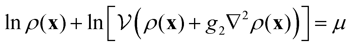where μ = ln(N/Z) is an effective chemical potential which can be thought as a Lagrange multiplier adjusting the total number of particles N in the system.²⁹ By using (7) in (8) and further expanding in gradients we havewhere .

Assuming a homogeneous density field ρ(x) = ρeqn (9) reduces to the fundamental equation describing MIPS at the mean-field level^30,31

Note that eqn (10) could have also been directly derived by assuming a homogeneous density in (3). Eqn (9) consistently shows that density gradients can also be neglected after the expansion.

For the choice of we now require that (i)eqn (10) admits a positive solution (ρ > 0) for any number of particles 0 < N < ∞ (i.e. for −∞ < μ < ∞) and that (ii)eqn (10) admits more than one positive solution, at least in some parameters range. A possible choice for , which satisfies (i) and (ii), is:

where and ρ₀ are positive parameters which control the response of the particle's speed to the density. According to (11) when a particle “perceives” a density much lower than the threshold density ρ₀ it moves fast (close to maximum speed ), while it moves almost at minimum speed () when ρ ≫ ρ₀. Property (i) is clearly satisfied by (11) since ln ρ ranges from −∞ to ∞ (as ρ varies between 0 and ∞) while stays finite. Property (ii) is fulfilled if ∂_ρμ < 0, i.e. if 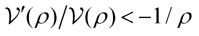(which is the condition for MIPS³⁰). Assuming that are fixed in (11), while is the control parameter, the system undergoes spinodal decomposition when

Moreover, by solving

we find that the spinodal line defined by (12) terminates in a critical point located at ρ_c = 3^1/2ρ₀ and as sketched in Fig. 1(a).

Fig. 1 (a) Theoretical spinodal curve (dashed line) in the mean field model of QS active particles. The system undergoes spinodal decomposition for large values of and intermediate values of ρ (blue area). The spinodal line terminates in a critical point (open square). (b) Coexistence region and critical point in AOUPs interacting via QS in d = 2 (numerical simulations). The system phase-separates for large values of and intermediate values of ρ (purple area). The estimated critical point is represented by an open circle. The critical point of the mean-field model in (a) is reported here for comparison (open square). (c)–(e) Snapshots of the largest system investigated (N = 30 × 10³ particles) at three different -values indicated in (b) along the critical density: a phase separated (c), a near-critical (d) and a homogeneous state point (e).

Interestingly the theory suggests that when particles react moving faster in low-density regions (i.e. when is increased above ) the system may phase separate, while particles always maintain a non-zero minimum speed also in the dense phase. Moreover an expansion of eqn (10) around the critical point shows that the latter belongs to the (mean-field) Ising universality class in full analogy with the condensation of van der Waals fluids.²⁹ In the following sections we will compare this scenario with the results of direct particle simulations in d = 2.

Numerical model and methods

Our microscopic model for QS is implemented by integrating eqn (1) and (2) for N identical point-like AOUPs (i.e., without excluded volume interactions). The speed of the i-th particle is computed as (see eqn (11)):
where the function g(x) is defined in eqn (5) and measures the local density within the cut-off distance R (which sets the range of the interaction). We fix all parameters of the active force to unity D = τ = 1, and the parameters of the QS interactions to ρ₀ = 1, and R = 1.3. The parameter , determining the speed change, will be varied to induce the phase separation and hence, together with density, it represents a control parameter of the system. Particles move in a rectangular box with periodic boundary conditions and with sides L_x = 3 × L_y. To apply the finite-size scaling analysis for the study of the critical point, we simulate different system sizes with N = (3.5, 7.5, 15, 30) × 10³. The equations of motion have been integrated numerically using the Euler scheme with a time step Δt = 10⁻³ up to N_t = 3 × 10⁸ time steps for the largest system size. To reach the stationary state a preliminary run has been performed for a comparable amount of steps, starting from a configuration in which particles are randomly distributed. As in ref. 13 we have checked that the auto-correlation function of density fluctuations relaxes for all system sizes within the simulation time window. Moreover, for each state point investigated, the whole procedure has been repeated five times starting from independent configurations.

To characterize the critical behavior of our model, we will rely on the finite-size scaling ansatz according to which any observable can be rewritten in terms of a dimensionless scaling function :

where is the critical exponent associated with the observable and ν is the exponent characterizing the divergence of the correlation length ξ, as the control parameter gets close to its critical value. As suggested by the mean-field theory described above, the speed change parameter can be used as a control parameter to tune the system at criticality and thus we assume . Note that the scaling ansatz (15) implies that, when the quantity is plotted as a function of , for different system sizes, all data should collapse onto the scaling function.

We are interested in measuring observables related to density fluctuations both for locating the critical point and estimating the critical exponents. These fluctuations are calculated using an improved version of the “block-density-distribution method” initially proposed by Binder and coworkers.^32–35 The technique represents an alternative to grand-canonical simulations (where the particle density fluctuates) to characterize density fluctuations in the canonical ensemble (where the overall density is fixed). The main idea is to divide the simulation box into small sub-boxes of linear size L that exhibit, to a good approximation, the same density fluctuations of the grand-canonical ensemble. In each sub-box one measures the particles number density ρ = N_b/L², where N_b is the number of particles found in a sub-box, and compute the density variance 〈Δρ²〉 = 〈(N_b/L²) − (〈N_b/L²〉)²〉 and its fourth moment 〈Δρ⁴〉 = 〈(N_b/L²) − (〈N_b/L²〉)⁴〉. From these quantities one then computes the “Binder cumulant” for which one expects that the ansatz (15) reduces to the simple form and thus, at the critical point, is size independent since This suggests that one could locate the critical point by finding the value of the control parameter at which the curves, for different sizes, cross. Unfortunately it has been shown that this procedure fails (the -curves do not cross) even for the equilibrium two-dimensional lattice gas in the canonical ensemble (which is equivalent to the Ising model with conserved magnetization).^16,35 The failure of this scheme can be attributed to the fact that the grand-canonical fluctuations cannot be well reproduced in the sub-boxes due to the large contribution coming from the interface between the two phases.

To overcome this problem, a modified version of the method has been proposed in ref. 16 and successfully applied both to critical equilibrium systems and active systems.^13,15–17 The basic idea of the modified method is that the system centre of mass can be used to locate the dense phase excluding the interfaces from the analysis. More specifically, for each particle configuration the x-coordinate of the systems’ centre of mass is always shifted to x = 3L_x/4 and density fluctuations are then evaluated far from the interface, by selecting only four squared sub-boxes of size L = L_y/2: two sub-boxes centred around x= 3L_x/4 (dense phase) and the other two in x = L_x/4 (dilute phase). The same procedure is then repeated for different system sizes to find the crossing of the cumulants and thus locate the critical point. It has been shown that this technique yields the correct critical point in d = 2 in the case of equilibrium square-lattice gas¹⁶ and the triangular-lattice gas.¹³

Note that by combining the sub-box method with the finite-size scaling formula (15) we can also obtain the values of the critical exponents. To this aim we employ the data-collapse optimization technique that has been previously exploited to extract critical exponents in various spin models.^36,37 To use this approach one first measures the variable at different values of the control parameter and of the system size. All collected measurements form a set of M data-points, where represent the i-th data point. If (15) holds, and the correct values of , and ν are known, the following quantity should be zero

where we have introduced the scaled variable . Note that the “error function” (16) is positive (i.e., since it is a sum of squares) and attains its minimum in the ideal case in which the critical parameters , and ν have their exact values. This implies that if we knew we could also minimize (16), with respect to , and ν to find their correct values, which is the basic principle that we will use in the data-analysis presented below. Although we generally do not know , we can still approximate it from the data. To this aim we divide the values in a set of W windows (with M > W) and average the values of the data-points lying within the same window. The value of appearing in (16) can then be calculated by a linear interpolation of the window-averaged . With this technique the function can be then minimized to obtain the parameters , ν and .

Results

Before focusing on the critical behavior we start by discussing how simulations results compare with the mean-field picture explained above. We first numerically locate the boundaries of the MIPS-region, by performing a numerical scan in ρ and for the smallest system size (N = 3500) distinguishing those state points in which phase-separation occurs from those in which the system is homogeneous. This has been done by checking whether the density distribution (computed over all sub-boxes) has two detectable peaks. The resulting coarse phase-diagram is reported in Fig. 1(b). Already from this data we can approximately locate the critical point to be at and ρ_c ≈ 3. Visual inspection of configurations immediately confirms that, upon increasing , QS active particles undergo a transition from a homogeneous state (Fig. 1(e)) to phase separation (Fig. 1(c)), with large fluctuations at intermediate -values (Fig. 1(d)). The overall picture confirms that the microscopic model follows qualitatively the mean-field scenario discussed above, albeit with significant quantitative differences. In particular, we observe that the MIPS of the numerical model occurs at significantly higher and ρ-values. However, the shape of the numerical coexistence curve is reminiscent of the theoretical spinodal line which is slightly asymmetric with the dense-fluid branch less steep than the gaseous one. To precisely locate the critical point we proceed as in ref. 13 calculating the Binder parameter , introduced in the previous Section, as a function of ρ and at fixed , i.e. near the critical . According to ref. 34, should exhibit a maximum at ρ = ρ_c when plotted as a function of the density at fixed . We perform this analysis for the smallest system size and, fitting the data with a parabola, we get the critical density ρ_c = 2.821(0.041) as shown in the inset of Fig. 2(a) (we report the fit error in the brackets). Since we are interested in the critical behavior of the system, from now on we will fix ρ = ρ_c for our analysis. To determine accurately the value of and of the exponent ν we first compute at different values of and L (simulation data are shown in Fig. 2(a)) and we minimize (16) with respect to ν and (which are considered as free fitting parameters). The optimization yields and ν = 1.040(0.045). We note that the exponents ν is close to the Ising value and that, when we use these parameters to scale data, we obtain a good collapse as shown in Fig. 2(b). Note also that, the obtained corresponds, to a good approximation, with the value at which the Binder cumulants cross, as shown by the vertical line in Fig. 2(a). The common crossing point of the Binder parameters at different L-values confirms that scale-invariance holds and thus that a critical point exists.³²

Fig. 2 (a) The main panel shows the Binder parameter obtained in simulations (data points) as function of for different system sizes (see legend). The full lines are fits with generalized logistic functions to guide the eye (also in (c) and (e)). The vertical line shows the value of the critical which is close to the intersection of the curves. The inset (same y-axis scale as main panel) shows the Binder parameter as a function of density (open symbols) computed in simulations with fixed = 18 and N = 3500. The position of the maximum is found by a fit with a parabola (full line) to estimate the critical density. (b) Collapse of the data in (a) with the parameters ν and determined by the optimization method. The full line is a fit of all data-points with the generalized logistic function as a guide to the eye (also in (d) and (f)). (c) susceptibility χ as a function of for different system sizes. (d) data of (c) collapsed with the critical exponent γ. (e) order parameter m vs for different system sizes. (f) collapsed data of (e) with the exponent β.

We now proceed to determine independently the exponents γ and β. To this aim, we fix the values of ν and to those found previously, letting as a free parameter in the optimization. To estimate γ we consider the susceptibility χ = 〈(N_b − 〈N_b〉)²〉/〈N_b〉 at different and L-values, as shown in Fig. 2(c). We then minimize (16) with respect to finding that γ = 1.763(0.070) (the error on ν is propagated), which is compatible with the Ising value. Data are well collapsed using this exponent as shown in Fig. 2(d). For estimating β we consider the order parameter m = ρ_dens − ρ_dil, defined as the difference between the densities of the dense (ρ_dens) and dilute (ρ_dil) phases.¹⁶ The values of m, collected at several and L, are shown in Fig. 2(e). The minimization of the error-function (16) with gives β = 0.116(0.013) (which is close to the Ising β = 0.125) and a scaling of data with this β provides a good collapse as shown Fig. 2(f). To conclude the analysis of the static critical exponents we now estimate the exponent η which controls the behavior of the critical static structure factor S(q) at low wave-vectors q. We consider , where ρ_q is the real part of the Fourier transform of the density field at time t: , where q = 2π(n_x/L_x,n_y/L_y) represents the wave-vector (n_x,y ∈ [Doublestruck Z]). Here we assume that rotational and time-translational invariance hold so that S(q) is averaged over all q with the same modulus q = |q| and over all times t. Moreover, the prefactor is chosen such that S(q → ∞) = 1. The S(q), calculated for the largest system size, is shown in Fig. 3 for two different -values across the transition. While far from the critical point the S(q) flattens at low q, close to the structure factor exhibits a power-law behavior. By fitting the low-q data with S(q) ∼ q^{−2 +η} we obtain 2 − η = 1.765(0.012), which is close to the Ising value (2 − η = 1.75). Note that the slope of the fit is appreciably different from the typical mean-field decay S(q) ∼ q⁻² which is also reported Fig. 2.

Fig. 3 Static structure factor S(q) computed for the largest system (N = 30 × 10³) at two state points with the same ρ = ρ_c but different (see legend). S(q) tends to a constant at low q in the homogeneous phase (blue points). Close to the critical point (orange data-points) the structure factor is well fitted, for small q values, by a power law S(q) ∼ q^−2+η (full line). The dashed line represents the fit with S(q) ∼ q⁻² (mean-field).

Finally, we focus on the critical dynamics of the QS system. As in ref. 14, we compute the time auto-correlation function C(q,t) = 2N⁻¹〈ρ_−q(t + s)ρ_q(s)〉 to characterize the dynamics of spontaneous fluctuations at different time- and length-scales. The C(q,t) is computed for various q-s and at the near-critical value . From correlations we compute the spectra . The functions ωC(q,ω) are shown in Fig. 4(a). We observe that ωC(q,ω) grows in amplitude upon lowering q and its peak shifts towards lower frequencies revealing the characteristic slowing-down of the system's dynamics at large length-scales. As discussed in ref. 14 the value of ω at which ωC(q,ω) reaches its maximum (denoted as ω_max) can be associated with the system's relaxation frequency at that q. Moreover in ref. 14 it was shown that AOUPs may exhibit deviations from the scaling regime at frequencies as high as the relaxation rate of the active force τ⁻¹ (appearing in the equations of motions (1) and (2)). For this reason, we restrict our analysis to q-values that are low enough so that ω_max ≪ 2π/τ.

Fig. 4 (a) Frequency-resolved correlation functions at various q values (see legend). (b) Scaling of the data in (a) by their amplitude and peak position. The green curve represents the scaled correlator from the equilibrium lattice gas. The dashed curve is the correlator from the Gaussian-field theory shown for comparison. (c) Peak frequency ω_max, from data in (a), plotted as a function of q (the error-bar on each data-point corresponds to the error made in fitting the peak position). The full line is a power-law fit to estimate the critical exponent z. The dashed line is the fit with the fixed exponent z = 4 (mean-field).

Within this q-range we first characterize the shape of ωC(q,ω). This is an interesting feature to consider since it is know³⁸ that, at the critical point, the relaxation spectrum C(q,ω) could be rewritten in terms of a universal scaling function as follows:

Eqn (17) implies that ω_max ∼ q^z and that all ωC(q,ω) should have the same shape described by . In Fig. 4(b) we check this by plotting data of Fig. 4(a) rescaled by their maxima, finding a good superposition. Moreover, since should be a universal scaling function we plot on top of our data the scaled ωC(q,ω) of the critical two-dimensional lattice gas in equilibrium (see ref. 14 and 39 for details). We find that the data of the QS active system follow quite well the correlator of the lattice gas simulations (especially at large ω/ω_max). Data are also compared with the result of the dynamical Gaussian field-theory³⁸ which yields ωC(q,ω) ∼ ω/(ω² + ω_max²). Fig. 4(b) shows that this formula (which should be valid only for d > 4) sensibly deviates from the data-points. As mentioned above we expect that the peak position follows ω_max ∼ q^z and this allows us to estimate the dynamic critical exponent z. In Fig. 4(c) we show ω_max as a function of q and the direct fit with a power-law giving z = 3.640(0.073) which is also compatible with z = 3.75 of the Ising model, with conserved magnetization and in d = 2. All exponents estimated in the present work are summarized in Table 1.

Table 1 Critical exponents estimated from simulations of the two-dimensional QS active system. The exponents of the Ising model with conserved magnetization are reported for comparison

Exponent	Ising value	Fitted value	Fit error
ν	1	1.040	0.045
γ	1.75	1.763	0.070
β	0.125	0.116	0.013
η	0.25	0.235	0.011
z	3.75	3.640	0.073

---

Conclusions

In this work we have investigated the critical behavior of an active system interacting via QS. In the model each particle senses the number of neighbors, within a given cut-off distance, and then varies its speed according to a specific rule. Mean-field theory suggests that this model has a spinodal line ending in a critical point. To check the validity of the theoretical picture we have performed large-scale numerical simulations on GPU, finding that the system does phase-separate and that the coexistence region terminates in a motility induced critical point. To address the problem of the universality class, we have used finite-size scaling analysis to measure static and dynamic critical exponents. We have found that these exponents are in substantial agreement with those of the two-dimensional Ising model with conserved magnetization.

We stress that, the QS system studied here interacts differently from the repulsive AOUPs of ref. 13. QS particles slow-down whenever they get close (independently of their orientation), which is different from repulsive active particles which slow-down (or even stop) only when pointing towards each other. Despite these differences the results for the critical fluctuations are nearly identical in these systems (which is the landmark of universality). We recall also that finite-size-scaling analysis has been applied to off-lattice¹⁶ and in-lattice simulations¹⁵ of repulsive ABPs with some controversial results. In particular the off-lattice simulations seem to lead to non-Ising exponents¹⁶ while on-lattice simulations seems to point towards the Ising universality class.¹⁵ Such an intense research motivates our present work on QS active particles for which a systematic study of the critical point has not been performed so far.⁴⁰ Our results on critical QS particles are also consistent with recent field theoretical developments.^41–43 Indeed, according to the derivation in ref. 42, only the presence of repulsive interactions, together with a density-dependent speed, could generate field-theoretical terms that may destabilize the critical point.

Our study also opens different possibilities for future investigations on critical active systems. It would be useful to understand if and how the QS interaction rules could be changed to possibly induce micro-phase separation. Moreover, it would be helpful to understand if and how the fluctuation dissipation theorem could be violated by critical QS particles. In particular, it could be to understand whether the breakdown of the theorem differs from the one observed for purely repulsive AOUPs.¹⁴ Finally, from a more general perspective, it would be interesting to compare the critical behavior of our QS system with the one of model systems interacting via chemotaxis,⁴⁴ in the presence of aligning^45,46 and/or steric interactions,⁴⁷ and in mixtures of active and passive particles.^48,49

Conflicts of interest

There are no conflicts of interest to declare.

References

1. M. B. Miller and B. L. Bassler, Annu. Rev. Microbiol., 2001, 55, 165–199.
2. K. H. Nealson, T. Platt and J. W. Hastings, J. Bacteriol., 1970, 104, 313–322.
3. J. Zhu, M. Miller, R. Vance, M. Dziejman, B. L. Bassler and J. J. Mekalanos, Proc. Natl. Acad. Sci. U. S. A., 2002, 99(5), 3129–3134.
4. B. Hammer and B. Bassler, Mol. Microbiol., 2003, 50(1), 101–104.
5. R. Daniels, J. Vanderleyden and J. Michiels, FEMS Microbiol. Rev., 2004, 28, 261–289.
6. J. R. Gomez-Solano, S. Samin, C. Lozano, P. Ruedas-Batuecas, R. van Roij and C. Bechinger, Sci. Rep., 2017, 7, 14891.
7. H.-R. Jiang, N. Yoshinaga and M. Sano, Phys. Rev. Lett., 2010, 105, 268302.
8. C. Maggi, J. Simmchen, F. Saglimbeni, J. Katuri, M. Dipalo, F. De Angelis, S. Sanchez and R. Di Leonardo, Small, 2016, 12, 446–451.
9. T. Bäuerle, A. Fischer, T. Speck and C. Bechinger, Nat. Commun., 2018, 9, 1–8.
10. F. Lavergne, H. Wendehenne and B. C. Bäuerle, Science, 2019, 364(6435), 70–74.
11. M. E. Cates and J. Tailleur, Annu. Rev. Condens. Matter Phys., 2015, 6, 219–244.
12. A. P. Solon, J. Stenhammar, M. E. Cates, Y. Kafri and J. Tailleur, Phys. Rev. E, 2018, 97, 020602.
13. C. Maggi, M. Paoluzzi, A. Crisanti, E. Zaccarelli and N. Gnan, Soft Matter, 2021, 17, 3807–3812.
14. C. Maggi, N. Gnan, M. Paoluzzi, E. Zaccarelli and A. Crisanti, Commun. Phys., 2022, 5, 55.
15. B. Partridge and C. F. Lee, Phys. Rev. Lett., 2019, 123, 068002.
16. J. T. Siebert, F. Dittrich, F. Schmid, K. Binder, T. Speck and P. Virnau, Phys. Rev. E, 2018, 98, 030601.
17. F. Dittrich, T. Speck and P. Virnau, Eur. Phys. J. E: Soft Matter Biol. Phys., 2021, 44, 1–10.
18. C. B. Caporusso, P. Digregorio, D. Levis, L. F. Cugliandolo and G. Gonnella, Phys. Rev. Lett., 2020, 125, 178004.
19. L. Caprini, U. M. B. Marconi, C. Maggi, M. Paoluzzi and A. Puglisi, Phys. Rev. Res., 2020, 2, 023321.
20. U. M. B. Marconi, M. Paoluzzi and C. Maggi, Mol. Phys., 2016, 114, 2400–2410.
21. E. Fodor, C. Nardini, M. E. Cates, J. Tailleur, P. Visco and F. van Wijland, Phys. Rev. Lett., 2016, 117, 038103.
22. U. Marini Bettolo Marconi, C. Maggi and M. Paoluzzi, J. Chem. Phys., 2017, 147, 024903.
23. S. Dal Cengio, D. Levis and I. Pagonabarraga, Phys. Rev. Lett., 2019, 123, 238003.
24. D. Martin, J. O’Byrne, M. E. Cates, É. Fodor, C. Nardini, J. Tailleur and F. van Wijland, Phys. Rev. E, 2021, 103, 032607.
25. H. Risken, The Fokker-Planck Equation, Springer, 1996, pp. 63–95.
26. C. W. Gardiner, et al., Handbook of stochastic methods, Springer, Berlin, 1985, vol. 3.
27. P. Hänggi and P. Jung, Adv. Chem. Phys., 1995, 89, 239–326.
28. L. Caprini, U. M. B. Marconi, R. Wittmann and H. Löwen, Soft Matter, 2022, 18, 1412–1422.
29. N. G. van Kampen, Phys. Rev., 1964, 135, A362–A369.
30. J. Tailleur and M. E. Cates, Phys. Rev. Lett., 2008, 100, 218103.
31. M. E. Cates and J. Tailleur, Annu. Rev. Condens. Matter Phys., 2015, 6, 219–244.
32. K. Binder, Z. Phys. B: Condens. Matter, 1981, 43, 119–140.
33. M. Rovere, D. Hermann and K. Binder, EPL, 1988, 6, 585.
34. M. Rovere, D. W. Heermann and K. Binder, J. Condens. Matter Phys., 1990, 2, 7009.
35. M. Rovere, P. Nielaba and K. Binder, Z. Phys. B: Condens. Matter, 1993, 90, 215–228.
36. S. M. Bhattacharjee and F. Seno, J. Phys. A: Math. Gen., 2001, 34, 6375.
37. J. Houdayer and A. K. Hartmann, Phys. Rev. B: Condens. Matter Mater. Phys., 2004, 70, 014418.
38. U. C. Täuber, Critical dynamics: a field theory approach to equilibrium and non-equilibrium scaling behavior, Cambridge University Press, 2014.
39. L. Caprini, F. Cecconi, C. Maggi and U. M. B. Marconi, Phys. Rev. Res., 2020, 2, 043359.
40. J. Stenhammar, arXiv, 2021, preprint, arXiv:2112.05024.
41. F. Caballero, C. Nardini and M. E. Cates, J. Stat. Mech.: Theory Exp., 2018, 2018, 123208.
42. C. Nardini, É. Fodor, E. Tjhung, F. Van Wijland, J. Tailleur and M. E. Cates, Phys. Rev. X, 2017, 7, 021007.
43. T. Speck, Phys. Rev. E, 2022, 105, 064601.
44. E. J. Marsden, C. Valeriani, I. Sullivan, M. Cates and D. Marenduzzo, Soft Matter, 2014, 10, 157–165.
45. F. Farrell, M. Marchetti, D. Marenduzzo and J. Tailleur, Phys. Rev. Lett., 2012, 108, 248101.
46. M. Paoluzzi, D. Levis and I. Pagonabarraga, arXiv preprint arXiv:2205.15643, 2022.
47. M. Paoluzzi, M. Leoni and M. C. Marchetti, Soft Matter, 2020, 16, 6317–6327.
48. J. Stenhammar, R. Wittkowski, D. Marenduzzo and M. E. Cates, Phys. Rev. Lett., 2015, 114, 018301.
49. D. R. Rodriguez, F. Alarcon, R. Martinez, J. Ramírez and C. Valeriani, Soft Matter, 2020, 16, 1162–1169.

---