DOI:
10.1039/D2SM00622G
(Paper)
Soft Matter, 2022,
18, 6868-6881
Non-equilibrium shapes and dynamics of active vesicles†
Received
13th May 2022
, Accepted 23rd August 2022
First published on 24th August 2022
Abstract
Active vesicles, constructed through the confinement of self-propelled particles (SPPs) inside a lipid membrane shell, exhibit a large variety of non-equilibrium shapes, ranging from the formation of local tethers and dendritic conformations, to prolate and bola-like structures. To better understand the behavior of active vesicles, we perform simulations of membranes modelled as dynamically triangulated surfaces enclosing active Brownian particles. A systematic analysis of membrane deformations and SPP clustering, as a function of SPP activity and volume fraction inside the vesicle is carried out. Distributions of membrane local curvature, and the clustering and mobility of SPPs obtained from simulations of active vesicles are analysed. There exists a feedback mechanism between the enhancement of membrane curvature, the formation of clusters of active particles, and local or global changes in vesicle shape. The emergence of active tension due to the activity of SPPs can well be captured by the Young–Laplace equation. Furthermore, a simple numerical method for tether detection is presented and used to determine correlations between the number of tethers, their length, and local curvature. We also provide several geometrical arguments to explain different tether characteristics for various conditions. These results contribute to the future development of steerable active vesicles or soft micro-robots whose behaviour can be controlled and used for potential applications.
1 Introduction
Many phenomena in biological cells, including cytoskeletal dynamics,1,2 cytoplasmic streaming,3 and cell migration,4,5 are intrinsically out of equilibrium.6 Such processes and functions inevitably rely on force generation by internal active elements, whose primary example is a filament-based cytoskeleton driven by the dynamic growth/shrinkage of its filaments and the activity of molecular motors.2,7,8 Non-equilibrium force generation by the cytoskeleton can lead to dynamic changes in cell shape, such as the formation of filopodia and lamellipodia9,10 and highly branched elongated structures in neurons and glia cells.11,12 Furthermore, non-equilibrium processes can contribute to different physical effects, such as active membrane fluctuations13,14 in cells, and the emergence of collective behavior within a group of biological or artificial microswimmers.15,16
To tackle the complexity of biological cells in a more systematic and controlled way, the field of synthetic biology has recently emerged.18,19 In particular, the bottom-up approach, where a synthetic cell is built from scratch by combining different cell-mimicking components,19,20 is appealing to physicists, as the composition and complexity of such systems can precisely be controlled. Examples include chemical factories that imitate different metabolic processes,21 membrane compartments with cytoskeletal filaments,22–24 and growth and spontaneous division of droplet-based or vesicle-based compartments.25,26 The development of cell mimics also includes artificial systems built from non-cell-derived components. One of the prominent examples is so-called active vesicles, which consist of a membrane enclosing active particles17,27–31 or filaments.32–34
A recent study combining experiments and simulations17 has realized active vesicles driven from inside by diffusiophoretic self-propelled particles (SPPs). Determined by the balance between forces exerted by active particles and membrane bending rigidity and tension, several different regimes of vesicle shapes are observed, see Fig. 1. For weak particle activity, SPPs cannot strongly deform the membrane, resulting in a quasi-spherical shape with active fluctuations. As the particle activity is increased at small to moderate particle densities, tethers are formed by single SPPs or their clusters. For large particle densities and high propulsion strengths of SPPs, bola-like and/or prolate vesicle shapes can form with two or more satellite vesicles. A similar active system has been realized by enclosing swimming bacteria inside a lipid vesicle, though the density of bacteria was kept relatively low.31
 |
| | Fig. 1 Phase diagram of various vesicle shapes, including fluctuating, tethering, and bola/prolate regimes, as a function of Peclet number Pe and the volume fraction ϕ of active particles. The solid black lines are the theoretical phase boundaries of the tethering regime. The grey region indicates the crossover between the fluctuating and the bola/prolate regimes. In all simulations of the phase diagram, the membrane area is conserved, while volume conservation is not imposed, so that the dimensionless area-to-volume ratio can adjust freely. Adapted from ref. 17. | |
The observed shapes of active vesicles, such as tethers, prolate and bola-like structures, as well as fluctuating quasi-spherical shapes, may have some resemblance with vesicle shapes in equilibrium, which are determined by the energy minimization for an imposed reduced volume and spontaneous curvature.35–37 For instance, a non-zero spontaneous curvature induced by the adsorption of amphipathic peptides or BAR domain proteins can lead to string-of-pearls-like and tubular protrusions,37,38 reminiscent of tether-like extensions of active vesicles. However, such structures in equilibrium are stationary and do not possess active force generation and dynamic shape changes, which occur in non-equilibrium systems driven by the underlying active processes. A recent example for a non-equilibrium vesicle system is the active shape oscillations of giant vesicles driven by dynamic changes in spontaneous curvature.39 For the case of vesicles with enclosed active particles, their highly dynamic shapes largely depend on the strength of active forces and their distribution, and the dynamics of the active components, so that fixed spontaneous curvature and reduced volume play at most a secondary role for such systems.17
Several physical mechanisms govern the behavior of active vesicles, including the curvature-induced clustering of active particles40 near the membrane, and generation of active tension through the swim pressure.41 The accumulation of active particles near the membrane is similar to wall accumulation of SPPs, which occurs due to a slow rotational diffusion so that SPPs spend a significant time at the walls.40,42 Local membrane curvature further enhances accumulation of SPPs at the membrane, and results in the formation of particle clusters, which are able to collectively alter the shape of active vesicles.17,27,29,30 At large enough SPP densities, motility-induced phase separation can also take place,43–45 leading to large clusters at the membrane surface. In order to better understand how far active vesicles are driven out of equilibrium, it is necessary to study the interplay between vesicle shape changes, local membrane properties, and the dynamics of active particles for various SPP densities and propulsion strengths.
In this study, we perform a systematic simulation investigation and analysis of active vesicle shapes and the clustering characteristics of SPPs. We demonstrate how varying particle activity and density strongly affect membrane properties such as local curvature and tension. Furthermore, changes in vesicle shapes are directly correlated with alterations in the dynamics and clustering of SPPs, resulting in a feedback mechanism between the enhancement of membrane curvature and the formation of active-particle clusters. In the tethering regime, the tether properties such as length and local curvature correlate with the number of tethers. Most of the non-equilibrium aspects of active vesicles can well be rationalized by simple theoretical arguments, providing a good explanation for the non-equilibrium behavior of active vesicles. A detailed understanding of and control over such systems is crucial toward the development of potential applications such as self-propelled soft micro-robots or synthetic cells with programmable functions.33,46–48
2 Methods and models
An active vesicle is represented by a closed fluid membrane of spherical topology with radius R, enclosing a number of active Brownian particles. The activity of the particles is described by the dimensionless Peclet number Pe = σvp/Dt, where σ is the particle diameter, vp the propulsion velocity, and Dt the translational diffusion coefficient. Note that Pe is a measure of the propulsion force fp of SPPs, with vp = fp/γp and Dt = kBT/γp, where γp is the translational friction coefficient, so that Pe = fpσ/kBT. Particle volume fraction within the vesicle is given by ϕ = Np(σ/2R)3, where Np is the number of enclosed SPPs. All simulation parameters are given in Table 1.
Table 1 Parameters used for 3D simulations of active vesicles both in model and physical units. Nt = 2Nv − 4 is the number of triangular faces in the vesicle discretization. Also, the table includes equilibrium value of local membrane curvature
| Parameters |
Model units |
Physical units |
|
Principal properties
|
| Vesicle radius in equilibrium R |
32 |
8 μm |
| Thermal energy unit kBT |
0.2 |
4.14 × 10⁻²¹ J |
| Time scale τ = γpR2/κc |
1.28 × 10⁵ |
7.3 s |
|
|
|
Investigated properties
|
| Peclet number Pe = σvp/Dt |
25–800 |
25–800 |
| Total number of SPPs Np |
3–1458 |
3–1458 |
| SPP volume fraction ϕ = Np(σ/2R)3 |
7.3 × 10⁻⁴–3.56 × 10⁻¹ |
7.3 × 10⁻⁴–3.56 × 10⁻¹ |
| SPP diameter σ |
R/8 |
1 μm |
|
|
|
Vesicle properties
|
| Number of vertices Nv |
30![[thin space (1/6-em)]](https://www.rsc.org/images/entities/char_2009.gif) 000 000 |
30000 |
| Bending rigidity κc |
20kBT |
8.28 × 10⁻²⁰ J |
| Average bond length lb |

|
0.176 μm |
| Bond stiffness kb |
80kBT |
3.31 × 10⁻¹⁹ J |
| Minimum bond length lmin |
0.6lb |
0.11 μm |
| Potential cutoff length lc1 |
0.8lb |
0.14 μm |
| Potential cutoff length lc0 |
1.2lb |
0.21 μm |
| Maximum bond length lmax |
1.4lb |
0.25 μm |
| Desired vesicle area A |
4πR2 |
8.04 × 102 μm2 |
| Desired vesicle volume V0 |
4πR3/3 |
2.14 × 103 μm3 |
| Local area stiffness ka |
6.43 × 10⁶kBT/A |
3.3 × 10⁻⁵ J m−2 |
| Volume stiffness kv (if used) |
1.6 × 10⁷kBT/R3 |
130 J m−3 |
| Friction coefficient γm |
0.4kBTτ/R2 |
1.9 × 10⁻¹⁰ J s m−2 |
| Flipping frequency ω |
6.4 × 10⁶τ−1 |
8.8 × 10⁵ s−1 |
| Flipping probability ψ |
0.3 |
0.3 |
|
|
|
SPP properties
|
| Translational friction γp |
20kBTτ/R2 |
9.4 × 10⁻⁹ J s m−2 |
| Translational diffusion Dt |
k
B
T/γp |
4.4 × 10⁻¹³ m2 s−1 |
| Rotational diffusion Dr |
3Dt/σ2 |
1.32 s−1 |
| LJ potential depth ε |
2kBT |
8.28 × 10⁻²¹ J |
|
|
|
Equilibrium vesicle properties
|
| Mean local curvature 〈Ceq〉 |
1.01R−1 |
0.126 μm−1 |
2.1 Model of self-propelled particles
SPPs are modeled as spherical active Brownian particles (ABPs) without hydrodynamic interactions. Each ABP experiences a propulsion force fp that acts along an orientation vector ei. The force results in a propulsion velocity 〈vp〉 = fp/γp, where γp is the friction coefficient. The orientation vector ei is subject to random rotation ėi = ζi × ei, where ζi is a Gaussian random process with 〈ζi(t)〉 = 0 and 〈ζi(t)ζj(t′)〉 = 2Drδijδ(t − t′) with a rotational diffusional coefficient Dr. Dr is related to the ABP size σ and translational diffusion coefficient Dt as Dt = Drσ2/3. Furthermore, the ABPs repel each other and the membrane, which is implemented through the repulsive part of the 12-6 Lennard-Jones potential, with the potential minimum at rm = σ for ABP-ABP interactions and rm = 0.5σ for ABP-membrane interactions. The potential cut-off is set at rc = 21/6rm, so that no attractive interactions are present.
2.2 Membrane model
The vesicle is modeled by a dynamically triangulated membrane of Nv linked vertices.49,50 The interaction between linked vertices is controlled via a tethering potential49,51 that is a combination of attractive and repulsive parts| |  | (1) |
| |  | (2) |
Here, kb is the bond stiffness, lmin and lmax are the minimum and maximum bond lengths, and lc0 and lc1 are the potential cutoff lengths.
The bending elasticity is modeled by the Helfrich curvature energy,52
| |  | (3) |
where
κc is the bending rigidity and
![[c with combining macron]](https://www.rsc.org/images/entities/i_char_0063_0304.gif)
is the mean local curvature at the membrane surface element d
A. In the discretized form, it becomes
53,54| |  | (4) |
where

is the discretized mean curvature at vertex
i,
![[n with combining right harpoon above (vector)]](https://www.rsc.org/images/entities/i_char_006e_20d1.gif) i
i is the unit normal at the membrane vertex
i,

is the area corresponding to vertex
i (the area of the dual cell),
j(
i) corresponds to all vertices linked to vertex
i, and
σij =
rij(cot
θ1 + cot
θ2)/2 is the length of the bond in the dual lattice, where
θ1 and
θ2 are the angles at the two vertices opposite to the edge
ij in the dihedral. In practice, since the dihedral terms corresponding to
σij are additive, the local curvature at each vertex can be calculated by summing over contributions from all triangles containing that vertex.
The area conservation is imposed locally to each triangle by the potential
| |  | (5) |
where
Nt = 2(
Nv − 2) is the number of triangles,
Al =
A0/
Nt is the targeted local area (
A0 is the total membrane area),
Ai is the instantaneous local area, and
ka is the local-area conservation coefficient. Also, there is a constraint applied on the total volume
V of the vesicle
via the potential
| |  | (6) |
where
kv is the volume constraint coefficient and
V0 is the desired total volume.
Membrane fluidity is modelled by a stochastic flipping of bonds following a Monte-Carlo scheme. The bond shared by each pair of adjacent triangles can be flipped to connect the two previously unconnected vertices.49,54 The flipping is performed with a frequency ω and probability ψ. An energetically favorable bond flip is accepted with a probability of p = 1. For an energetically unfavorable flip, the resulting change in energy due to an attempted bond flip ΔU = ΔUatt + ΔUrep + ΔUA determines the probability of the flipping as ψ = exp[−ΔU/kBT]. The resulting membrane fluidity can be characterized by a 2D membrane viscosity for the selected frequency ω and flipping probability ψ.51,55
2.3 Equation of motion
The system evolves in time according to the Langevin equation| |  | (7) |
where m is the mass of membrane particle or SPP,  and ri represent the second and first time derivatives of particle positions, ∇i is the spatial derivative at particle i, and Utot is the sum of all interaction potentials described above. The effect of a viscous fluid is mimicked by the friction co-efficient γ, whose value can be different for membrane particles and SPPs. Thermal fluctuations are modelled as a Gaussian random process ξi with 〈ξi(t)〉 = 0 and 〈ξi(t)ξj(t′)〉 = δijδ(t − t′). Inertial effects are minimized by performing the simulations in the over-damped limit with m and γ such that τt = m/γ < 1 ≪ τr = Dr−1. The positions and velocities of all particles are integrated using the velocity-Verlet algorithm.56
3 Results
3.1 Dynamic vesicle shapes
In the absence of volume constraint at Pe = 0 (i.e., passive particles), the vesicle has a nearly spherical shape with thermal membrane fluctuations for the entire range of volume fractions ϕ. As Pe is increased, active fluctuations appear in addition to the thermal undulations, representing the fluctuating regime (see Fig. 1). However, in the fluctuating regime for Pe ≲ 100, the average shape of the vesicle remains nearly spherical, independently of ϕ, since the propulsion force of SPPs or their clusters is too weak to induce tethering or dramatic changes in the vesicle shape. For Pe ≳ 100 and ϕ ≲ 0.1, dynamic tether formation becomes possible by single SPPs or their clusters. At Pe ≳ 100 and large enough ϕ ≳ 0.1, several large clusters of SPPs may form at the membrane, which can pull in different directions and induce a spontaneous symmetry breaking to prolate and bola-like shapes. Note that the shapes in the prolate/bola regime are also very dynamic.
Due to the rotational diffusion of the SPPs and the dynamic adjustment of membrane shape in reaction to the pushing forces generated by the active particles, vesicle shapes are highly dynamic (e.g., persistent tether formation and retraction). This is illustrated in Fig. 2 and corresponding Movie S1 (ESI†). Tether formation starts when the orientation of a SPP is essentially along the membrane normal. For times t ≲ τr = 1/Dr, the SPP moves ballistically and pulls a straight tether. The particle velocity slows down with increasing tether length, as the friction imposed by the tether increases linearly with tether length. At times t ≃ τr, the pulling direction of the SPP starts to deviate from the initial tether orientation, resulting in tether curving as it elongates further. Now, the retraction force of the tether given by κ/Rb (Rb is the tether radius) in the absence of a membrane tension shortens the tether length by pulling it toward a straight configuration. At the same time, the anchoring point of the tether at the vesicle may move in the force direction. Finally, on even larger time scale t > τr, there is a significant probability that the propulsion direction of the SPP reverts toward the vesicle surface, so that the SPP would move back through the tether accompanied by tether retraction.
 |
| | Fig. 2 Several snapshots of a simulation illustrating tether pulling and retraction for parameters Pe = 400, ϕ = 0.002 and a reduced volume ν = 0.8. (a and b) For t < τr, SPPs move ballistically and pull a few tethers. (c) When t ≃ τr, SPPs start changing their direction of propulsion which leads to tether curving. (d) For t > τr, some of the tethers are retracted since some SPPs may move back toward the vesicle. (e and f) For SPP clusters, some particles continuously leave and join different tethers. See also Movies S1 (ESI†). | |
When there are more than one SPP in the tether, the dynamics becomes even richer, as shown in Fig. 2(e) and (f) and Movie S1 (ESI†). In addition to several SPPs pulling together to extend the tether, some active particles may have changed their orientation at times t > τr, and either move back along the tether or on their way back to the vesicle pull in a direction roughly perpendicular to the tether orientation, thereby inducing a kink in the tether shape or a branching of the tether.
In order to characterize and understand this non-equilibrium behavior and the resulting dynamic shapes of active vesicles, we perform a detailed analysis of their various properties. Note that the analysis of the membrane properties and particle clustering focuses on simulations without a volume constraint, whereas for the analysis of tethers, simulations both with and without a volume constraint are considered.
3.2 Vesicle membrane characteristics
3.2.1 Local curvature.
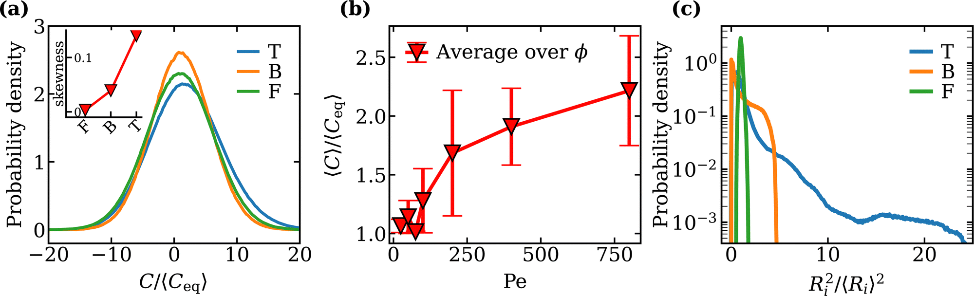
Fig. 3(a) shows distributions of the reduced local curvature ![[C with combining macron]](https://www.rsc.org/images/entities/i_char_0043_0304.gif) = C/〈Ceq〉 for different activities and classes of vesicle shapes, where 〈Ceq〉 is the average local mean curvature measured from an equilibrium simulation of the vesicle, i.e. with no enclosed active particles. The distributions indicate considerable variations in the local curvature induced by thermal fluctuations of the membrane and changes in the vesicle shape due to SPPs. The distribution peak for the “fluctuating” phase is centered at 〈Ceq〉 ≃ 1/R, and shifts towards larger values from the fluctuating to the tethering regime. The tethering regime is associated with the development of regions with a high curvature. This leads to a non-zero skewness 〈(C − 〈C〉)3〉/〈(C − 〈C〉)2〉3/2 of the distribution, as shown in the inset of Fig. 3(a). In the ‘bola’ regime, the distribution of local curvature is narrower than for the other cases due to smaller fluctuations of the vesicle. In this case, membrane fluctuations become suppressed as a result of high density of SPPs and the development of significant active tension.27,28
= C/〈Ceq〉 for different activities and classes of vesicle shapes, where 〈Ceq〉 is the average local mean curvature measured from an equilibrium simulation of the vesicle, i.e. with no enclosed active particles. The distributions indicate considerable variations in the local curvature induced by thermal fluctuations of the membrane and changes in the vesicle shape due to SPPs. The distribution peak for the “fluctuating” phase is centered at 〈Ceq〉 ≃ 1/R, and shifts towards larger values from the fluctuating to the tethering regime. The tethering regime is associated with the development of regions with a high curvature. This leads to a non-zero skewness 〈(C − 〈C〉)3〉/〈(C − 〈C〉)2〉3/2 of the distribution, as shown in the inset of Fig. 3(a). In the ‘bola’ regime, the distribution of local curvature is narrower than for the other cases due to smaller fluctuations of the vesicle. In this case, membrane fluctuations become suppressed as a result of high density of SPPs and the development of significant active tension.27,28
 |
| | Fig. 3 (a) Local curvature distributions for the tethering (T) (Pe = 200, ϕ = 0.02), bola (B) (Pe = 200, ϕ = 0.18) and fluctuating (F) (Pe = 25, ϕ = 0.06) regimes. The inset shows the effect of global shape changes on the skewness 〈(C − 〈C〉)3〉/〈(C − 〈C〉)2〉3/2 of the distributions. (b) Mean local curvature 〈C〉 as a function of Pe. The values are averaged over different ϕ with ϕ < 0.18. (c) Distribution for the squared distances 〈Ri2〉/〈Ri〉2 of the membrane from the vesicle center of mass for the tethering, bola and fluctuating regimes. The tail is pronounced for the bola and tethering regimes with the latter having a significantly slow decay. | |
At low ϕ, an increase in Pe causes a transition from the fluctuating to the tethering regime. Tethers are regions of a high curvature due to their small radii, causing an overall increase in the mean local curvature 〈C〉. Consequently, the transition into the tethering regime at Pe ∼ 100 is accompanied by a steep increase in 〈C〉, as shown in Fig. 3(b). Note that the values of 〈C〉 at each Pe are averaged over various ϕ values lying in the fluctuating and tethering regimes, i.e. ϕ < 0.18.
3.2.2 Squared distance from the center of mass.
To differentiate between active vesicles in the tethering regime and in the fluctuating/bola regimes, a useful quantity is the squared distance Ri2/〈Ri〉2 of the membrane vertices from the center-of-mass of the vesicle. This quantity characterizes well a deviation of the vesicle shape from a sphere, as tethers cause the mean value of Ri2/〈Ri〉2 to increase. Fig. 3(c) shows that the distribution in the tethering regime is significantly wider than those in the bola and fluctuating regimes. Furthermore, the distribution for the tethering regime exhibits a pronounced tail due to the formation of multiple long tethers. The distribution for the bola regime also has a tail, although it decays much faster than that in the tethering case. The distribution for the fluctuating regime is nearly symmetric with no significant tails.
3.2.3 Membrane tension.
The membrane tension λ of active vesicles can be divided into two contributions: active and passive (equilibrium) tension, i.e. λ = λa + λeq. The passive tension is computed as the membrane tension (see Appendix A) for an equilibrium simulation of the vesicle at ϕ = 0 (i.e., no SPPs), and is close to zero for a vesicle in equilibrium, i.e. λ = λeq ≃ 0. Even though λeq ≃ 0, it is not exactly zero due to numerical errors and approximations used in the calculations. Therefore, only the deviations from the equilibrium are considered for the membrane tension, knowing that the tension of the vesicle in equilibrium is zero.57,58 In the presence of active particles, the membrane tension increases and is generated as a consequence of the swim pressure41 due to the active Brownian particles.
For a fixed Pe, an increase in particle density ϕ leads to a linear increase in the vesicle tension, as shown in Fig. 4(a). However, Peclet number affects the slope, so that it increases with increasing Pe, and saturates for Pe > 100. A similar effect on membrane tension is observed for a fixed particle density, when Pe is increased, see Fig. 4(b). The dependence of λ on Pe is also linear with a slope nearly independent of ϕ.
 |
| | Fig. 4 Linear increase in the reduced vesicle tension ![[small lambda, Greek, macron]](https://www.rsc.org/images/entities/i_char_e0cc.gif) as a function of (a) ϕ and (b) Pe. The values of the vesicle tension are normalized as = λ/λ0, with λ0 = R2kBT/(πσ4), and have further been re-scaled by the corresponding value of ϕ and Pe. The solid lines are linear fits to the data. as a function of (a) ϕ and (b) Pe. The values of the vesicle tension are normalized as = λ/λ0, with λ0 = R2kBT/(πσ4), and have further been re-scaled by the corresponding value of ϕ and Pe. The solid lines are linear fits to the data. | |
To better understand these trends, we estimate the active tension originating from the swim pressure via the Young–Laplace equation as
| |  | (8) |
where
χ ≤ 1 is the active tension weight which accounts for deviations of the particle force direction from orientation along the membrane normal. Its value changes with both Pe and
ϕ,
i.e. χ =
χ(Pe,
ϕ). With the proportionality Pe ∝
fp and
ϕ ∝
Np, the active tension can be described as
| | | = χPeϕ, | (9) |
where
=
λ/
λ0 is the vesicle tension normalized by
λ0 =
R2kBT/(π
σ4). This theoretical argument supports the linear dependence of
λ in
Fig. 4(a) and (b) obtained from simulations.
To investigate the dependence of χ on the parameters involved, we determine the fraction ρ of SPPs located at the membrane for different Pe and ϕ. ρ is calculated as the number of particles Np,mem, which are in direct or indirect contact with the membrane (within a distance of 1.75σ, i.e. accounting for up to three layers of SPPs), divided by the total number of SPPs as ρ = Np,mem/Np. All values of ρ are averaged over 10 statistically independent timeframes of simulations. The values of χ are obtained by fitting a linear function in eqn (9) to the data in Fig. 4(a) and (b). Note that in general, it is difficult to decouple the effects of Pe and ϕ on χ. As an approximation, we use χ(Pe,ϕ) ≃ χ(Pe,ϕ0) for the variation of with ϕ, where ϕ0 is an unknown parameter which minimizes the function  . This approximation allows us to qualitatively extract the effect of different Pe on χ by measuring the slope χ(Pe,ϕ0). The same method can be employed for the variation of with Pe.
Fig. 5(a) and (c) shows that both χ and ρ follow similar trends as a function of Pe, suggesting that the larger is the particle fraction at the membrane, the larger the contribution of SPPs to active tension. Note that for low particle densities ϕ < 0.005, χ can be larger than unity [see Fig. 5(a)], because the distribution of SPPs at the membrane is very inhomogeneous, which makes the analysis based on the Young–Laplace equation questionable. However, for ϕ ≳ 0.005, χ values remain in the range between 0.7 and 1.0, indicating that the majority of SPPs exert a force along a direction close to the normal direction of the membrane. This is due to the fact that the rotational diffusion of SPPs is small (or Pe is large), so that the SPPs primarily push in the direction of the membrane normal. Fig. 5(b) and (c) shows that nearly all SPPs are located at the membrane for large Pe, independently of ϕ. However, at low Pe and large ϕ, a considerable fraction of SPPs remain away from the membrane, as the SPPs are able to leave the membrane due to larger rotational diffusion (low Pe). Moreover, at low Pe, most SPPs can never reach the membrane surface due to the comparable effects of diffusion and propulsion.
 |
| | Fig. 5 (a) Dependence of the active tension weight χ on Pe and ϕ. The values of χ are obtained using a linear fitting of the function = χPeϕ. Variation in fraction ρ of SPPs located at the membrane surface as a function of (b) Pe and (c) ϕ. The value of ρ is calculated as the number of particles Np,mem that are in a direct or indirect contact with the membrane divided by the total number of particles, i.e., ρ = Np,mem/Np. | |
3.3 Active particle clustering
The mobility of SPPs and the membrane-mediated interactions lead to the formation of particle clusters. We perform the analysis of cluster sizes and their dependence on Pe and ϕ. Furthermore, the mobility of single SPPs is characterized by their fixed-time displacements, and the shape of clusters is described through cluster asphericity.
3.3.1 Cluster sizes.
Clusters of SPPs are identified by using a clustering algorithm, where particles located within a cutoff distance rcut are considered as a part of the same cluster. In this analysis, rcut is selected to be 1.1σ. Fig. 6(a) and (b) presents the distributions of cluster sizes for different Pe and ϕ. At low ϕ, only small clusters with sizes of Nc ≃ 10 are formed due to a limited number of particles. Nevertheless, an increase in Pe leads to a larger probability to form larger clusters as seen in Fig. 6(a), since at low ϕ, particles primarily cluster at membrane locations with significant deformation (or large local curvature). SPPs simply spend more time at the locations of large membrane curvature due to longer escape times, so that large curvatures promote SPP accumulation and clustering. This process can also be described as a feedback-loop mechanism, where the arrival of additional particles to a cluster generates larger cluster forces which result in stronger membrane deformation, aiding SPP accumulation and cluster growth. Fig. 6(b) also shows a secondary peak in the cluster-size distribution at large enough ϕ ≳ 0.1. At large ϕ, SPPs cover a substantial portion of the membrane area, yielding a few large clusters in the prolate regime. Note that, even though small clusters are still present at large ϕ, their probability reduces in comparison to the cases with low ϕ, since the majority of SPPs is located within the large clusters.
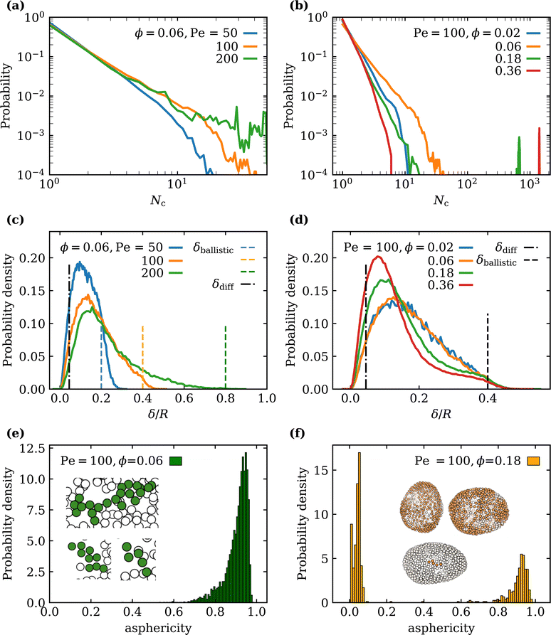 |
| | Fig. 6 Distributions of various SPP cluster properties. Cluster-size distributions (a) for different Pe at ϕ = 0.06 and (b) for different ϕ at Pe = 100. Fixed-time displacement δ/R distributions, characterizing SPP mobility for various (c) Pe and (d) ϕ for Δt = 0.1Dr−1. Estimates based on diffusive (dashed dotted lines) and ballistic motion (dotted lines) of the SPPs are plotted for reference. Cluster asphericity distributions at Pe = 100 for (e) ϕ = 0.06 and (f) ϕ = 0.18. The insets show snapshots of particle clusters near the vesicle membrane (particle size is not to scale). | |
3.3.2 SPP mobility.
In order to determine changes in particle mobility as a function of Pe and ϕ, the fixed-time displacement δ of SPPs is computed as a distance traveled by each active particle during a fixed time interval Δt = 0.1τr. For a free SPP in three dimensions, the crossover time t* from the diffusive to the ballistic regime can be estimated as t* ≃ 18τr/Pe2. For Pe = 100, this implies Δt ≃ 54t* which is well beyond the diffusive regime, with an expected fixed time displacement| |  | (10) |
The results in Fig. 6(c) and (d) suggest that while a small fraction of SPPs exhibits ballistic motion (indicated by the distribution tail in Fig. 6(d)), the majority of SPPs moves much slower than a free active particle due to the interactions of SPPs with the membrane and each other. The slowing down of SPPs occurs due to their small rotational diffusion such that when the SPP is near the membrane, the orientation vector of the particle mostly points in the direction of the membrane normal. An approximation based on two-dimensional diffusion of a SPP at the membrane surface yields the estimate| |  | (11) |
which is still significantly lower than the distribution peaks in Fig. 6(c) and (d). Thus, despite a considerable slowing down of the SPPs at the vesicle membrane, the fixed-time displacements are on average larger than δdiff due to SPP activity. The value of Pe does not significantly affect the peak of δ distributions [see Fig. 6(c)], but mainly alters the distribution tail.
For a fixed Pe, an increase in ϕ shifts the peak of mobility distribution to lower values of δ [see Fig. 6(d)], as the lateral mobility along the membrane surface becomes hindered due to steric repulsion between SPPs within large clusters. Note that the distributions for ϕ = 0.02 and ϕ = 0.06 in Fig. 6(d) are nearly identical, as the cluster sizes for the both particle densities are small and lie within a similar range (Nc ∈ (1,40)). As the cluster size grows with increasing ϕ [see Fig. 6(a)] for a fixed Pe, the lateral mobility of SPPs decreases. Therefore, the results in Fig. 6(c) and (d) suggest that the average cluster sizes determine the peak position of the mobility distribution, while the value of Pe affects the distribution tail.
3.3.3 Cluster shapes.
We characterize cluster shapes by their asphericity, as defined in Appendix B. Clusters whose asphericity is close to zero have a near-spherical shape, whereas asphericity close to unity implies a rod-like shape. Note that only clusters with more than four particles are taken into consideration in this analysis. Fig. 6(e) and (f) shows a strong dependence of the cluster-shape distribution on particle density for Pe = 100 (fluctuating regime). For low particle densities (ϕ ≲ 0.06), most clusters have an elongated shape; nearly all particles have a direct contact with the membrane surface, so that only single-layer flat clusters of sizes in the range Nc∈ (5,30) are formed as seen in the insets of Fig. 6(e). At large SPP densities (ϕ ≳ 0.18), large clusters develop, see Fig. 6(a), whose shape is closer to a filled sphere, as they generally consist of several layers of SPPs and are distributed over a considerable area of the vesicle, see the insets of Fig. 6(f). However, several small clusters with Nc ∼ 10 may still be present at large ϕ, whose asphericity is close to unity as in the case for low particle densities. Therefore, asphericity distribution in Fig. 6(f) has two peaks at large ϕ. For ϕ = 0.36, almost all clusters have near zero asphericity, since hardly any small clusters remain.
3.4 Membrane tethers
Membrane tethers are detected by using an automated algorithm based on the positions of membrane vertices and SPPs, as described in Appendix C. Various tether properties, such as tether size, length, curvature and number, are calculated from simulations both with and without volume constraints.
3.4.1 Tether length distribution.
Fig. 7 presents a distribution of tether lengths Lteth, which are computed from simulation data as the distance between the vertices in the tether closest and farthest away from the vesicle center of mass. Since active vesicles are highly dynamic and the tethers constantly change their length, the data are collected every Δt = 0.1τr within a time frame 0.4τr < t < 5τr from simulations representing the tethering regime with Pe ∈ (50,800). Note that the range of Pe starts from a lower value than the critical Pe for tether formation in the state diagram in Fig. 1, because simulation data for other reduced volumes, where tether formation may occur at a lower Pe,17 are also included in the analysis.
 |
| | Fig. 7 Tether length distribution obtained from simulations and a simple model with an assumption that Lteth,th = α1Pet* + α2, where α1 and α2 are fitting parameters. | |
To rationalize the computed distribution of Lteth, a simple model of linear tether growth is considered as
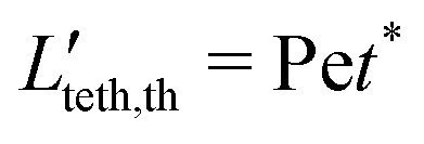
| | | Lteth,th = α1Pet* + α2, | (12) |
where
α1 accounts for multiple factors such as tether friction and effective pulling force of the SPPs due to clustering and varying propulsion direction,
α2 represents the existence of a minimum tether length required for the automated algorithm to detect it, and
t* ∈ [0,1] is the dimensionless time. First, we randomly sample the lengths

for various Pe ∈ (50,800) and
t* ∈ [0,1]. Then, the required coefficients
α1 and
α2 are calculated as

and
, where std(*) denotes standard deviation. Finally, the estimated tether lengths are given by
. Note that in this model, the range of
t* can be taken arbitrarily as
α1 absorbs any scaling of the time, and
α2 accounts for a minimum tether length so that
t* can start from zero. However, this is not true for the selection of Pe values, as changing the range of Pe causes a qualitative change in the distribution of
Lteth,th.
Fig. 7 shows a very good agreement between the distributions computed from the simulation data and the model above, suggesting that the linear tether extension model provides a reasonable description for the tether growth and captures the principal mechanism.
3.4.2 Geometrical estimates of tether curvature and length as a function of its size.
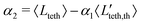
To rationalize dependencies between various tether properties, two classes of tethers are assumed. For tethers formed by less than 10 SPPs, the front (or head) of a tether is relatively small and can be neglected in comparison with a long cylindrical stalk. Such tethers are characterized by the radius Rb of the cylindrical stalk. For tethers formed by large clusters, we can assume that the head constitutes the major part of the tether, while the cylindrical stalk can be neglected. These tethers are characterized by the radius Rh of the tether head. For a cylindrical tether, the radius in equilibrium is determined by the vesicle tension λ as59 , where κc is the membrane bending rigidity. The particle diameter σ is another length scale that is relevant for tether formation; however, it should not affect the radius Rb of the stalk for long enough tethers. The average equilibrium tether radius can now be estimated as
 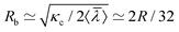 , where the calculated mean vesicle tension 〈〉 ≃ 1.9λ0 is averaged over all simulations with tethers. Note that Rb decreases with increasing Pe, as membrane tension increases. Also, it is important to mention that there is a minimal tether radius in our simulations, which is determined by the bond length lb of the discretized membrane; this corresponds to Rb ≳ lb ≃ R/45.
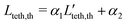
In addition, we define the tether size as the number of vertices Nv,teth within the tether which is proportional to the area of the tether Ateth as Nv,teth = B1Ateth. The constant B1 can be calibrated through the relation between the total number of vertices in the membrane and the total membrane area A as B1 = Nv/A = 2387R−2. Fig. 8(a) presents the relation between the average local curvature 〈Cteth〉 of the tether and tether size, which is well described by a power law. The value of the power-law exponent can be estimated through dimensional analysis. For tethers formed by clusters with Nc < 10, Nv,teth ∼ Rb and 〈Cteth〉 ∼ Rb−1, implying a power-law dependence 〈Cteth〉 ∼ Nv,teth−1. However, for tethers formed by large clusters, Nv,teth ∼ Rh2, so that 〈Cteth〉 ∼ Nv,teth−0.5. This rather crude approximation qualitatively captures the dependence of 〈Cteth〉 on tether size in Fig. 8(a) with an exponent of 0.9 for tethers formed by less than 10 particles and an exponent of 0.4 for tethers formed by more than 10 particles.
 |
| | Fig. 8 (a) Mean local tether curvature 〈Cteth〉/Ceq as a function of tether size Nv,teth. The various colors represent tethers formed by SPP clusters of different sizes. The solid black line is a fit for tethers formed by clusters with Nc < 10, while the dashed black line is for tethers formed by clusters with Nc > 10. The lines are least-squared fits to the data using the function 〈Cteth〉/Ceq = ANv,teth−B + C, whose form is motivated by the geometrical arguments in Section 3.4.2. (b) Variation of the tether size Nv,teth with tether length Lteth for tethers formed by clusters with Nc < 10. The solid line is a linear fit to the data based on eqn (13). (c) Mean vesicle curvature 〈C〉/Ceq as a function of the number Nteth of detected tethers. The black line indicates the best fit, while the gray region is the confidence interval computed using a bootstrap procedure. | |
For tethers with less than 10 SPPs, a positive linear correlation of tether length with size is presented in Fig. 8(b). We assume that the “head” of cylindrical tethers on average has a constant size, which implies a fixed offset. We then obtain the equation
| |  | (13) |
where
Lteth is the tether length. We assume that
Rb ≃ 2
R/32 and
S1 =
B1(2π
Rb)
R ≃ 30
R.
Rh ≃ 〈
Nc〉
1/3σ/2 ≃ 3.6
R/32 is determined by considering that on average clusters of size 〈
Nc〉 occupy the tether head, where we have used 〈
Nc〉 = 3.2 as determined from the simulation data. Then,
S2 =
B1(4π
Rh(
Rh −
Rb)) ≃ 170 can be estimated. The linear fit based on the determined slope
S1 and intercept
S2 is presented in
Fig. 8(b) and follows well the simulation data.
3.4.3 Average membrane curvature with number of tethers.
Fig. 8(c) shows the mean local curvature averaged over the whole vesicle as a function of the number of tethers. Here, the number of tethers and the curvature are averaged over every Δt = 0.1τr, as the active system is highly dynamic and a single snapshot is not sufficient for the analysis. A positive linear correlation of the mean curvature with the number of tethers is found, since the tethers are regions of enhanced local curvature. The slope of the linear fit in Fig. 8(c) can be estimated as follows. With the assumption that all tethers have some mean length 〈Lteth〉, a mean radius Rh and Rb for the tether head and body respectively, the average mean local curvature 〈C〉 of the vesicle can be expressed as| | 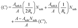 | (14) |
where Nteth is the number of tethers, A = 4πR2 is the total vesicle area, Ateth,b = 2πRb(〈Lteth〉 − 2Rh) is the area of the tether body, Ateth,h = 4πRh2 is the area of the tether head, Ateth = Ateth,b + Ateth,h is the total tether area, and 〈C′〉 is the average mean local curvature of the reduced main vesicle body with area A′ = 4πR′2 = A − AtethNteth. In the limit of AtethNteth/A ≪ 1, eqn (14) reduces to| |  | (15) |
where 〈Ceq〉 = 1/R is the equilibrium mean vesicle curvature. The values of 〈Lteth〉 = 0.53R (measured from the distribution of lengths), Rb ≃ 2R/32 (estimated from the calculated mean vesicle tension 〈〉 ≃ 1.9λ0 averaged over all simulations with tethers) and Rh = 6R/32 (estimated from the calculated mean cluster size 〈Nc〉 ≃ 9), imply the slope and the value of 〈C〉/〈Ceq〉 at Nteth = 0 to be 0.2 and unity, respectively. A least squares fit to the data in Fig. 8(c) results in the values of 0.19 and 0.99, which agree very well with the estimate above. Note that despite the tether number, radius, and length being very dynamic quantities, this theoretical argument based on averages captures the data very well.
4 Summary and conclusions
Unlike static vesicle shapes obtained in equilibrium through energy minimization, active vesicles exhibit highly dynamic shape changes such as persistent tether formation and retraction. Therefore, active vesicles require a statistical physics approach, where stationary states of such systems and the variability in system properties can be characterised by the corresponding distributions and their moments. We have performed simulations and a systematic analysis of structural and dynamic properties of vesicles with enclosed active particles. Distributions of local curvature and the departure of vesicle geometry from a spherical shape are strongly affected by the non-equilibrium nature of this active system. As a result, dramatic and dynamic changes in vesicle shape have a substantial effect on its membrane properties. For instance, there exists a direct relation between active tension of the vesicle and the fraction of SPPs located at the membrane surface, which can be quantified via the Young–Laplace equation. Furthermore, enhanced local curvature of the vesicle favors the accumulation of SPPs, leading to a feedback loop between the evolution of local curvature and particle accumulation. This has been confirmed through the analysis of dynamic SPP clustering at the membrane, including variations in particle displacement, cluster size and shape as a function of Pe and ϕ. At ϕ ≲ 0.1 and large enough Pe, small SPP clusters with Nc ∼ 10 are formed, and trigger the formation of various tether structures. At large particle densities, the cluster size distribution develops the second peak due to the formation of very large SPP clusters which cover a substantial area of the membrane. Note that when large clusters are formed, the number of small clusters generally becomes reduced. The formation of large clusters is similar to the motility-induced phase separation found in non-equilibrium systems of active particles.45,60 Distributions of particle mobility suggest a competition between SPP activity leading to an increase in the lateral mobility of particles along the membrane surface and steric repulsion between SPPs, which plays an increasing role in the formation of large clusters. Finally, we have employed an automated method for tether detection, which allows a subsequent analysis of tether number, size, shape, and local curvature for different simulated conditions. Most of the correlations between different tether properties can be rationalized by considering two classes of tether geometries: (i) tethers with a long cylindrical body whose head can be omitted, and (ii) tethers with a large head formed by a cluster of SPPs. The distribution of tether lengths can be rationalized well by considering a linear growth model of the tethers for a given range of Pe. These theoretical arguments provide qualitative understanding of tether structure and variability.
Despite the fact that most of the non-equilibrium aspects of active vesicles can well be rationalized, several observations still remain unclear. The analysis of SPP mobility at the membrane surface shows that the lateral motion of active particles is majorly diffusive. This raises an interesting question whether motility-induced phase separation can take place under certain conditions and how the local curvature of the membrane influences the possible coexistence of low-density and high-density phases. Furthermore, it would be interesting to study the effects of particle shape and hydrodynamic interactions on the behavior of active vesicles, as such systems can be a precursor for active synthetic micro-robots capable of performing specific functions. For instance, the ability to change shape and induce membrane deformations is of importance for the motility of active systems,33,46 the internalization of drug-delivery particles by cells,61 and the development of biomimetic systems which can mimic phagocytic functions.48
Author contributions
G. G. and D. A. F. conceived the research project. P. I. performed the simulations and analysed the obtained data. All authors participated in the discussions and writing of the manuscript.
Conflicts of interest
There are no conflicts to declare.
Appendix A: calculation of membrane tension
Membrane tension is calculated using the virial theorem.62 We consider the three contributions: forces from global volume constraint, local area conservation and bond stretching/compression. The contributions from the bending energy and global area conservation are not considered for membrane tension, because the bending forces mainly act perpendicular to the tension plane while the global area coefficient has been set to zero in the simulations. The stress tensor τα,β for a system of N particles contained in a volume V is defined via the virial theorem as| |  | (16) |
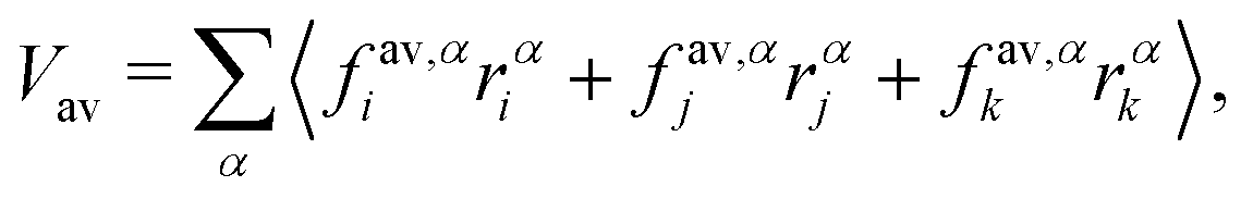
where fi is the net force on particle i due to inter-particle interactions and α, β are the coordinates x, y or z. Since the stress is written as sum over all particles, an atomic/local stress tensor τi,α,β can be defined, which characterizes the local stress at the particle i. Note that the local stress is the same as the stress throughout the system, and appropriate spatial and temporal averages must be performed for the equivalence between the virial stress and the mechanical stress. Since our system has both two-body and three-body interactions, the determination of the local stress tensor is not immediately obvious. However we are only interested in the trace of the stress tensor, which in two dimensions characterizes the tension of the vesicle. The sum over virial contributions from three body forces (area/volume constraints) is given by| | 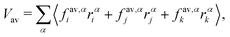 | (17) |
where indices i, j and k correspond to the vertices of the triangle and fav,αi is the force on vertex i in the direction α due to the area and volume constraints. This contribution is then divided equally between the three vertices. For bond forces fb,αi and fb,αj acting on vertices i and j, the virial contribution Vb is divided equally among the two vertices and is calculated as| | 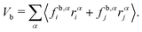 | (18) |
The total virial contribution from particle forces at each vertex is therefore V = Vav/3 + Vb/2. The tension in the system is calculated as a spatial and temporal average of the local stresses| |  | (19) |
where the factor two is due to the dimensionality of the system, Vi(t) is the virial contribution at vertex i at time t due to inter-particle forces and ai is the area of the dual cell, which is approximated by considering that each neighbouring triangle to the vertex contributes roughly one-third to the area. The contribution from momentum transfer is approximated by using the equipartition theorem.
Appendix B: asphericity of SPP clusters
Cluster shapes are quantified by their asphericity. The asphericity is calculated from the gyration tensor G, which is based on the second moments of N particle positions as| |  | (20) |
where r is measured from the center of mass of the N-particle system, i.e. . Let λ1, λ2, and λ3 be the eigenvalues of G. Then, the asphericity A is defined as63
| |  | (21) |
Values of A range between 0 and 1, with A = 0 for a perfectly spherical shape, and A = 1 for a long rod.
Appendix C: tether detection
For the detection and analysis of membrane tethers, we have developed an automated algorithm based on the positions of membrane vertices and SPPs. First, an adaptive cutoff distance from the center of mass of a vesicle is defined as| | 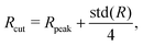 | (22) |
where Rpeak and std(R) are the peak position and standard deviation of the distance distribution of membrane vertices from the vesicle center of mass, respectively. Vertices that are located beyond this cutoff may belong to a tether. The coefficient 1/4 in front of std(R) is chosen by a trial-and-error procedure such that a large fraction of tethers is retained, while the detection of non-tether-like membrane undulations is minimized. Note that a too large cutoff may exclude the base region of tethers. An adaptive threshold is necessary as a single cutoff value fails to properly detect tethers in different simulations due to a significant complexity of active vesicle shapes. Then, a density-based clustering algorithm is used to determine membrane regions which represent different tethers.
After the identification of possible tether regions, false tether detections have to be eliminated. First, existing SPP clusters are identified and only membrane regions that are associated with some SPP clusters are retained. This association is made if the distance between the membrane patch and a SPP cluster is within a cutoff distance of 2.2R/32 (compare to the particle radius of σ/2 = 2R/32). In this step, no minimum cluster size is defined, so that even single SPPs are considered as clusters. This is a valid assumption since even single active particles are able to pull tethers at large enough Pe. The association of SPP clusters with possible tether regions does not guarantee that those regions are tethers, as enhanced membrane undulations are induced by active particles. Therefore, in the second check, the standard deviation σj = std(Ri) of a possible tether region j (Ri are vertex distances from the vesicle's center of mass) is considered. For non-tether-like membrane undulations, a low standard deviation is expected, because such regions are typically flat with moderate deviations from the mean value 〈Ri〉. However, for a tether, a number of vertices will lie considerably above and below the mean 〈Ri〉, leading to a large standard deviation. As a rule of thumb, only regions with σj > 2.5R/32 are retained as possible tethers, and this cutoff value of σj was selected manually to minimize false detection.
Finally, the last check is performed to eliminate ‘global’ shape changes of a vesicle misidentified as tethers. These are typically very large regions with a high tension due to a large number of SPPs near them. Such membrane regions are eliminated by considering the ‘size’ of such regions Nv,teth using a selected threshold of Nv,teth < 104, i.e. we impose an order of magnitude restriction based on the total size of the vesicle Nv = 3 × 10⁴ which ensures that the identified region is not a ‘global’ shape change. We also restrict the algorithm for ϕ < 0.18 to avoid the bola/prolate regime. Fig. 9 illustrates this multistep procedure for the detection of tethers, which allows us to automatically identify tethers in most simulations. Other properties of identified tethers such as mean tension, size of the associated cluster, tether length and tether size, can then easily be computed.
 |
| | Fig. 9 Illustration of tether identification. (a) A vesicle shape with tethers. (b) Several regions identified as possible tethers based on an adaptive cutoff distance from the center of mass of the vesicle. (c) Identification of tethers by discarding non-tether-like (e.g., due to membrane undulations) regions. | |
Acknowledgements
We thank Thorsten Auth and Roland G. Winkler for many helpful discussions. The authors gratefully acknowledge the computing time granted through JARA on the supercomputer JURECA64 at Forschungszentrum Jülich.
Notes and references
- L. Blanchoin, R. Boujemaa-Paterski, C. Sykes and J. Plastino, Physiol. Rev., 2014, 94, 235–263 CrossRef CAS PubMed.
- M. Kelkar, P. Bohec and G. Charras, Curr. Opin. Cell Biol., 2020, 66, 69–78 CrossRef CAS PubMed.
- R. E. Goldstein and J.-W. van de Meent, Interface Focus, 2015, 5, 20150030 CrossRef PubMed.
- K. M. Yamada and M. Sixt, Nat. Rev. Mol. Cell Biol., 2019, 20, 738–752 CrossRef CAS PubMed.
- A. Shellard and R. Mayor, Trends Cell Biol., 2020, 30, 852–868 CrossRef CAS PubMed.
- X. Fang, K. Kruse, T. Lu and J. Wang, Rev. Mod. Phys., 2019, 91, 045004 CrossRef CAS.
- M. W. Kirschner, J. Cell Biol., 1980, 86, 330–334 CrossRef CAS PubMed.
- U. S. Schwarz and M. L. Gardel, J. Cell Sci., 2012, 125, 3051–3060 CAS.
- P. K. Mattila and P. Lappalainen, Nat. Rev. Mol. Cell Biol., 2008, 9, 446–454 CrossRef CAS PubMed.
- M. Krause and A. Gautreau, Nat. Rev. Mol. Cell Biol., 2014, 15, 577–590 CrossRef CAS PubMed.
- L. A. Lowery and D. Van Vactor, Nat. Rev. Mol. Cell Biol., 2009, 10, 332–343 CrossRef CAS PubMed.
- D. M. Suter and K. E. Miller, Prog. Neurobiol., 2011, 94, 91–101 CrossRef CAS PubMed.
- Y.-K. Park, C. A. Best, T. Auth, N. S. Gov, S. A. Safran, G. Popescu, S. Suresh and M. S. Feld, Proc. Natl. Acad. Sci. U. S. A., 2010, 107, 1289–1294 CrossRef CAS PubMed.
- H. Turlier, D. A. Fedosov, B. A. Audoly, T. Auth, N. S. Gov, C. Sykes, J.-F. Joanny, G. Gompper and T. Betz, Nat. Phys., 2016, 12, 513–519 Search PubMed.
- M. C. Marchetti, J. F. Joanny, S. Ramaswamy, T. B. Liverpool, J. Prost, M. Rao and R. A. Simha, Rev. Mod. Phys., 2013, 85, 1143–1189 CrossRef CAS.
- J. Elgeti, R. G. Winkler and G. Gompper, Rep. Prog. Phys., 2015, 78, 056601 CrossRef CAS PubMed.
- H. R. Vutukuri, M. Hoore, C. Abaurrea-Velasco, L. van Buren, A. Dutto, T. Auth, D. A. Fedosov, G. Gompper and J. Vermant, Nature, 2020, 586, 52–56 CrossRef CAS PubMed.
-
Nat. Biotechnol., 2009, 27, 1071–1073, https://doi.org/10.1038/nbt1209-1071 Search PubMed.
- P. Schwille, J. Spatz, K. Landfester, E. Bodenschatz, S. Herminghaus, V. Sourjik, T. J. Erb, P. Bastiaens, R. Lipowsky, A. Hyman, P. Dabrock, J.-C. Baret, T. Vidakovic-Koch, P. Bieling, R. Dimova, H. Mutschler, T. Robinson, T.-Y. D. Tang, S. Wegner and K. Sundmacher, Angew. Chem., Int. Ed., 2018, 57, 13382–13392 CrossRef CAS PubMed.
- D. Needleman and Z. Dogic, Nat. Rev. Mater., 2017, 2, 17048 CrossRef CAS.
- T. Beneyton, D. Krafft, C. Bednarz, C. Kleineberg, C. Woelfer, I. Ivanov, T. Vidakovic-Koch, K. Sundmacher and J.-C. Baret, Nat. Commun., 2018, 9, 2391 CrossRef PubMed.
- F. C. Keber, E. Loiseau, T. Sanchez, S. J. DeCamp, L. Giomi, M. J. Bowick, M. C. Marchetti, Z. Dogic and A. R. Bausch, Science, 2014, 345, 1135–1139 CrossRef CAS PubMed.
- E. Loiseau, J. A. M. Schneider, F. C. Keber, C. Pelzl, G. Massiera, G. Salbreux and A. R. Bausch, Sci. Adv., 2016, 2, e1500465 CrossRef PubMed.
- K. Jahnke, M. Weiss, C. Weber, I. Platzman, K. Göpfrich and J. P. Spatz, Adv. Biosyst., 2020, 4, 2000102 CrossRef CAS PubMed.
- K. Weirich, K. L. Dasbiswas, T. A. Witten, S. Vaikuntanathan and M. L. Gardel, Proc. Natl. Acad. Sci. U. S. A., 2019, 116, 11125–11130 CrossRef CAS PubMed.
- J. Steinkühler, R. L. Knorr, Z. Zhao, T. Bhatia, S. M. Bartelt, S. Wegner, R. Dimova and R. Lipowsky, Nat. Commun., 2020, 11, 905 CrossRef PubMed.
- M. Paoluzzi, R. Di Leonardo, M. C. Marchetti and L. Angelani, Sci. Rep., 2016, 6, 34146 CrossRef CAS PubMed.
- J. Chen, Y. Hua, Y. Jiang, X. Zhou and L. Zhang, Sci. Rep., 2017, 7, 15006 CrossRef PubMed.
- Y. Li and P. R. ten Wolde, Phys. Rev. Lett., 2019, 123, 148003 CrossRef CAS PubMed.
- C. Wang, Y. Guo, W. Tian and K. Chen, J. Chem. Phys., 2019, 150, 044907 CrossRef PubMed.
- S. C. Takatori and A. Sahu, Phys. Rev. Lett., 2020, 124, 158102 CrossRef CAS PubMed.
- M. S. Peterson, A. Baskaran and M. F. Hagan, Nat. Commun., 2021, 12, 1–9 CrossRef PubMed.
- C. Abaurrea-Velasco, T. Auth and G. Gompper, New J. Phys., 2019, 21, 123024 CrossRef.
- H. Ni and G. A. Papoian, J. Phys. Chem. B, 2021, 125, 10710–10719 CrossRef CAS PubMed.
- U. Seifert, K. Berndl and R. Lipowsky, Phys. Rev. A: At., Mol., Opt. Phys., 1991, 44, 1182 CrossRef CAS PubMed.
- S. Svetina and B. Žekš, Eur. Biophys. J., 1989, 17, 101–111 CrossRef CAS PubMed.
- R. Lipowsky, Faraday Discuss., 2013, 161, 305–331 RSC.
- R. Lipowsky, Adv. Colloid Interface Sci., 2022, 102613 CrossRef CAS PubMed.
- S. Christ, T. Litschel, P. Schwille and R. Lipowsky, Soft Matter, 2021, 17, 319–330 RSC.
- Y. Fily, A. Baskaran and M. F. Hagan, Soft Matter, 2014, 10, 5609–5617 RSC.
- S. C. Takatori, W. Yan and J. F. Brady, Phys. Rev. Lett., 2014, 113, 028103 CrossRef CAS PubMed.
- J. Elgeti and G. Gompper, Europhys. Lett., 2013, 101, 48003 CrossRef CAS.
- J. Tailleur and M. E. Cates, Phys. Rev. Lett., 2008, 100, 218103 CrossRef CAS PubMed.
- M. E. Cates and J. Tailleur, Annu. Rev. Condens. Matter Phys., 2015, 6, 219–244 CrossRef CAS.
- P. Digregorio, D. Levis, A. Suma, L. F. Cugliandolo, G. Gonnella and I. Pagonabarraga, Phys. Rev. Lett., 2018, 121, 098003 CrossRef CAS PubMed.
- M. Medina-Sánchez, V. Magdanz, M. Guix, V. M. Fomin and O. G. Schmidt, Adv. Funct. Mater., 2018, 28, 1707228 CrossRef.
- A. Deblais, T. Barois, T. Guerin, P.-H. Delville, R. Vaudaine, J. S. Lintuvuori, J.-F. Boudet, J.-C. Baret and H. Kellay, Phys. Rev. Lett., 2018, 120, 188002 CrossRef CAS PubMed.
- Y. Sato, Y. Hiratsuka, I. Kawamata, S. Murata and S. M. Nomura, Sci. Rob., 2017, 2, eaal3735 CrossRef PubMed.
-
G. Gompper and D. M. Kroll, Statistical mechanics of membranes and surfaces, World Scientific, Singapore, 2nd edn, 2004, pp. 359–426 Search PubMed.
- D. M. Kroll and G. Gompper, Science, 1992, 255, 968–971 CrossRef CAS PubMed.
- H. Noguchi and G. Gompper, Phys. Rev. E: Stat., Nonlinear, Soft Matter Phys., 2005, 72, 011901 CrossRef PubMed.
- W. Helfrich, Z. Naturforsch., C: J. Biosci., 1973, 28, 693–703 CrossRef CAS PubMed.
- G. Gompper and D. M. Kroll, J. Phys. I, 1996, 6, 1305–1320 CrossRef.
- G. Gompper and D. M. Kroll, J. Phys.: Condens. Matter, 1997, 9, 8795–8834 CrossRef CAS.
- H. Noguchi and G. Gompper, Phys. Rev. Lett., 2004, 93, 258102 CrossRef PubMed.
-
M. P. Allen and D. J. Tildesley, Computer simulation of liquids, Clarendon Press, New York, 1991 Search PubMed.
- R. Goetz and R. Lipowsky, J. Chem. Phys., 1998, 108, 7397–7409 CrossRef CAS.
- F. David and S. Leibler, J. Phys. II, 1991, 1, 959–976 CrossRef CAS.
- I. Derényi, F. Jülicher and J. Prost, Phys. Rev. Lett., 2002, 88, 238101 CrossRef PubMed.
- A. Wysocki, R. G. Winkler and G. Gompper, Europhys. Lett., 2014, 105, 48004 CrossRef.
- S. Dasgupta, T. Auth and G. Gompper, Nano Lett., 2014, 14, 687–693 CrossRef CAS PubMed.
- D. H. Tsai, J. Chem. Phys., 1979, 70, 1375–1382 CrossRef CAS.
- J. Rudnick and G. Gaspari, J. Phys. A: Math. Gen., 1986, 19, L191–L193 CrossRef.
- Jülich Supercomputing Centre, J. Large-Scale Res. Facil., 2021, 7, A182 CrossRef.
Footnote |
| † Electronic supplementary information (ESI) available: A movie of an active vesicle illustrating tether pulling and retraction. See DOI: https://doi.org/10.1039/d2sm00622g |
|
| This journal is © The Royal Society of Chemistry 2022 |
Click here to see how this site uses Cookies. View our privacy policy here. 
 Open Access Article
 This Open Access Article is licensed under a
  ,
Gerhard
Gompper
,
Gerhard
Gompper


 is the discretized mean curvature at vertex i,
  is the area corresponding to vertex i (the area of the dual cell), j(i) corresponds to all vertices linked to vertex i, and σij = rij(cot


 and ri represent the second and first time derivatives of particle positions, ∇i is the spatial derivative at particle i, and Utot is the sum of all interaction potentials described above. The effect of a viscous fluid is mimicked by the friction co-efficient γ, whose value can be different for membrane particles and SPPs. Thermal fluctuations are modelled as a Gaussian random process ξi with 〈ξi(t)〉 = 0 and 〈ξi(t)ξj(t′)〉 = δijδ(t − t′). Inertial effects are minimized by performing the simulations in the over-damped limit with m and γ such that τt = m/γ < 1 ≪ τr = Dr−1. The positions and velocities of all particles are integrated using the velocity-Verlet algorithm.56


 . This approximation allows us to qualitatively extract the effect of different Pe on χ by measuring the slope χ(Pe,ϕ0). The same method can be employed for the variation of


 for various Pe ∈ (50,800) and t* ∈ [0,1]. Then, the required coefficients α1 and α2 are calculated as
  and
and  , where std(*) denotes standard deviation. Finally, the estimated tether lengths are given by
 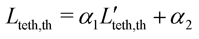 . Note that in this model, the range of t* can be taken arbitrarily as α1 absorbs any scaling of the time, and α2 accounts for a minimum tether length so that t* can start from zero. However, this is not true for the selection of Pe values, as changing the range of Pe causes a qualitative change in the distribution of Lteth,th. Fig. 7 shows a very good agreement between the distributions computed from the simulation data and the model above, suggesting that the linear tether extension model provides a reasonable description for the tether growth and captures the principal mechanism.
 , where κc is the membrane bending rigidity. The particle diameter σ is another length scale that is relevant for tether formation; however, it should not affect the radius Rb of the stalk for long enough tethers. The average equilibrium tether radius can now be estimated as
  , where the calculated mean vesicle tension 〈


 . Let λ1, λ2, and λ3 be the eigenvalues of G. Then, the asphericity A is defined as63

