DOI:
10.1039/D2SM00063F
(Paper)
Soft Matter, 2022,
18, 3771-3780
Arrested coalescence of multicellular aggregates†
Received
12th January 2022
, Accepted 22nd March 2022
First published on 5th May 2022
Abstract
Multicellular aggregates are known to exhibit liquid-like properties. The fusion process of two cell aggregates is commonly studied as the coalescence of two viscous drops. However, tissues are complex materials and can exhibit viscoelastic behaviour. It is known that elastic effects can prevent the complete fusion of two drops, a phenomenon known as arrested coalescence. Here we study this phenomenon in stem cell aggregates and provide a theoretical framework which agrees with the experiments. In addition, agent-based simulations show that active cell fluctuations can control a solid-to-fluid phase transition, revealing that arrested coalescence can be found in the vicinity of an unjamming transition. By analysing the dynamics of the fusion process and combining it with nanoindentation measurements, we obtain the effective viscosity, shear modulus and surface tension of the aggregates. More generally, our work provides a simple, fast and inexpensive method to characterize the mechanical properties of viscoelastic materials.
Shaping of organs during morphogenesis results from the material response of the constituent tissues to the forces which in turn are generated by them. Understanding the material properties of biological tissues holds the key to elucidating how shape and form emerge during morphogenesis both in vivo during embryonic development,1,2 as well as in vitro in the context of synthetic morphogenesis.3–5 For instance, viscous dissipation allows tissues to gradually change their shape without accumulation of significant stresses6,7 and adapt to different environments. Embryonic tissues are known to exhibit liquid-like properties: they round up,8,9 fuse,10 engulf other tissues11 and segregate or sort from heterotypic cell mixtures.12,13 However, tissues are also known to exhibit elastic behaviour which can critically affect the final tissue configuration.8,9,14 Unlike viscous forces, which only affect the rate of deformation of the tissue, elastic forces can resist deformation leading to a non-trivial final tissue configuration. Indeed jamming14 and viscoelastic8,15 effects have been shown to be critical in different morphogenetic processes.
The mechanical properties of tissues have been measured using a wide range of techniques (for a detailed review see ref. 16 and 17). Absolute measurements of tissue mechanical parameters such as surface tension γ, viscosity η or shear modulus μ, are possible by means of different techniques such as parallel plate compression,8,18,19 axisymmetric drop shape analysis,9,20 micropipette aspiration21 and drop sensors.22,23 In all cases, an external force is used to probe the system. A few methods have been used to obtain relative measurements at the tissue scale such as laser ablation24 or the fusion of multicellular aggregates.25–27 In both cases the measured velocities can be related to material properties. In the first case, the strain rate is related to the ratio of tissue stress σ and viscosity η,24 while in the second case the speed of fusion is dictated by the viscocapillary velocity γ/η.26,28–31 Of all the previous methods, limited appreciation has been given to the fusion method,10,27,32,33 which is arguably one of the simplest methods to obtain relative measures. Additional advantages of the method are the fact that there is no need for a calibrated probe and it is a non-contact method.16 The fusion of viscoelastic droplets is known to exhibit a phenomenon known as arrested coalescence,34–37 whereby the degree of coalescence is related to the elasticity of the material. The stable anisotropic shapes it can produce, have been exploited extensively to produce emulsions in a wide range of industries like food, cosmetics, petroleum and pharmaceutical formulations.34–36,38,39 Interestingly, this phenomenon has also been observed in biological tissues,40,41 as well as other active matter systems such as ant42 or bacterial43 aggregate colonies. Despite the fact that the sintering of drops is a classical problem that has been extensively studied both for passive28–30,44–46 and active systems,26,31,42,43,47,48 arrested coalescence still remains poorly understood.
In this work, we study the phenomenon of arrested coalescence in stem cell aggregates and show that a minimal Kelvin–Voigt model successfully captures the dynamics of the process. By fitting our model to the fusion dynamics, the viscocapillary velocity vc = γ/η and the shear elastocapillary length ![[small script l]](https://www.rsc.org/images/entities/char_e146.gif) e = γ/μ49 can be obtained. In addition, we complement these results with nanoindentation measurements to obtain absolute values of the effective viscosity, shear modulus and surface tension of the aggregates. Finally, by using agent-based simulations of the fusion process, we propose a mechanism by which active cell fluctuations can drive a solid-to-fluid phase transition and explore how the supracellular mechanical properties arise from the cell level interactions.
e = γ/μ49 can be obtained. In addition, we complement these results with nanoindentation measurements to obtain absolute values of the effective viscosity, shear modulus and surface tension of the aggregates. Finally, by using agent-based simulations of the fusion process, we propose a mechanism by which active cell fluctuations can drive a solid-to-fluid phase transition and explore how the supracellular mechanical properties arise from the cell level interactions.
1 Experimental setup
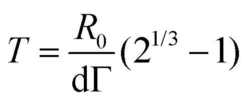
Fusion experiments were carried out by placing two cellular aggregates in contact with each other (Fig. 1A and B). In Fig. 1C an example of the fusion of two aggregates of mouse embryonic stem cells is shown. Arrested coalescence was observed after ∼4 h (Fig. 1C and Movie S1, ESI†), with anisotropic shapes maintained for the next ∼6 h. During the fusion process, the aggregates increased in size due to cell proliferation. To quantify the change in radius we imaged the growth of single aggregates. The radius of the aggregates increased linearly over time. After ∼4 h, the radius of the aggregates increased by ≃5%, corresponding to a ≃15% increase in volume (Fig. S1, ESI†). The doubling time of the cells was estimated by simply fitting a linear function to the time evolution of the aggregate radius (see Appendix) and was found to be T = 13.8 ± 0.4 h (n = 10, mean ± SD). Given that the fusion process is ∼3 times faster than cell division, we conclude that the volume of the cell aggregates does not change significantly during the fusion process.
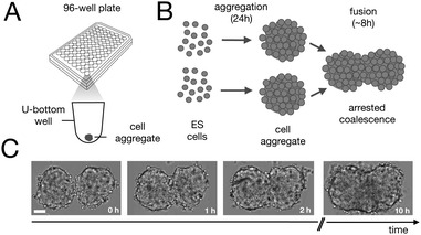 |
| | Fig. 1 Arrested coalescence in aggregates of mouse embryonic stem cells. (A) Spheroids were formed by aggregation of embryonic stem cells in low adhesion U-bottom multiwell plates. (B) Cell aggregates were placed in close contact at 24 h after aggregation and the fusion process was imaged using bright field microscopy. (C) Image sequence of a fusion event showing the resulting anisotropic shape of the assembly. Notice that the anisotropic shape of the assembly does not change significantly from ∼2 h to 10 h. Scale bar: 50 μm. | |
2 Continuum model
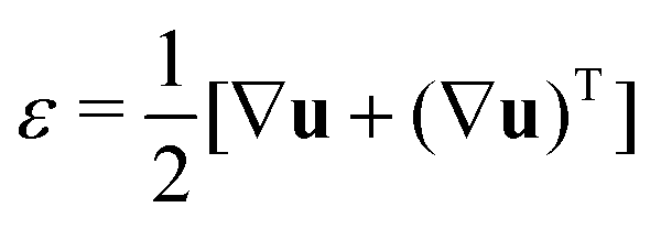
In order to understand the fusion dynamics, we considered each multicellular aggregate as a drop of a homogeneous incompressible Kelvin–Voigt material with effective shear viscosity η, shear modulus μ and surface tension γ. Kelvin–Voigt type models have been shown to be successful in describing the relaxation dynamics of multiple types of embryonic tissue explants19 and cellular spheroids,9 and they are arguably the simplest models to describe arrested coalescence.36 Given the fact that there is no apparent order in our aggregates, we will neglect an active anisotropic stress contribution considered in other studies.48 The constitutive equation for the stress tensor σ is then σ = 2η![[small epsi, Greek, dot above]](https://www.rsc.org/images/entities/i_char_e0a1.gif) + 2με − PI, where
+ 2με − PI, where  is the symmetric strain tensor, P is the hydrostatic pressure and u is the displacement field. Given that cell proliferation is negligible on the timescale of fusion, we approximate the continuity equation as ∇·
![[u with combining dot above]](https://www.rsc.org/images/entities/b_char_0075_0307.gif) = 0. Force balance in the bulk and on the surface read ∇·σ = 0 and σ·n = 2γHn, respectively, where H is the local mean curvature of the surface and n is the unit normal vector to the surface. Notice that in general η, μ, γ or P will depend on cell activity. Next, following the work in ref. 28–31, we approximate the assembly as two identical spherical caps of radius R(θ) with a circular contact ‘neck’ region of radius r(θ) = R(θ)
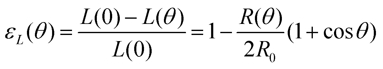
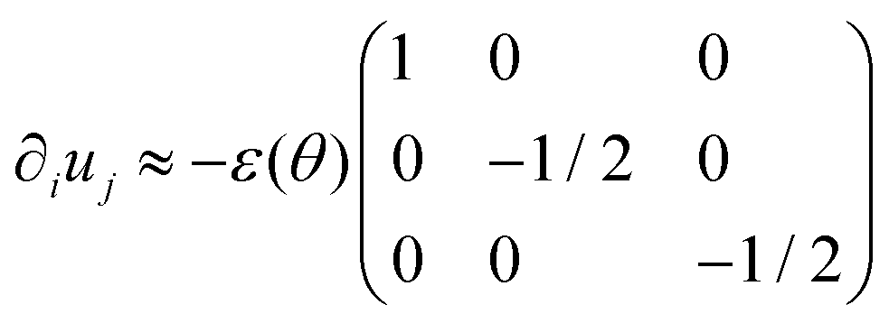
= 0. Force balance in the bulk and on the surface read ∇·σ = 0 and σ·n = 2γHn, respectively, where H is the local mean curvature of the surface and n is the unit normal vector to the surface. Notice that in general η, μ, γ or P will depend on cell activity. Next, following the work in ref. 28–31, we approximate the assembly as two identical spherical caps of radius R(θ) with a circular contact ‘neck’ region of radius r(θ) = R(θ)![[thin space (1/6-em)]](https://www.rsc.org/images/entities/char_2009.gif) sinθ, with a fusion angle θ (Fig. 2A). The dependence of the radius R on θ is determined by the incompressibility condition (see Appendix). The dynamics of the fusion process will be described by the evolution of θ(t). Let us assume the axis of fusion to be ex (Fig. 2A). The end-to-end length L(θ) of the fusion assembly along this axis will be given by L(θ) = 2R(θ)(1 + cosθ). It is known that coalescence of viscoelastic solid drops can be suppressed for sufficiently large values of the elastic modulus.36 The physics at the onset of fusion is not captured by our hydrodynamic model and has its origin on the cell–cell interactions between the two aggregates. To account for such an effect we incorporate an ad hoc yield strain by considering a shift of the rest length L′(0) = L(0) + δL, being δL/L(0) ≪ 1. In this way, we include a minimum critical strain that needs to be overcome to trigger coalescence, as proposed in ref. 36. The strain is approximated as ∂xu ≃ − ε(θ), with ε(θ) = [L′(0) − L(0)]/L′(0) ≃ εY + εL(θ), where εY = δL/L′(0) is the yield strain and
sinθ, with a fusion angle θ (Fig. 2A). The dependence of the radius R on θ is determined by the incompressibility condition (see Appendix). The dynamics of the fusion process will be described by the evolution of θ(t). Let us assume the axis of fusion to be ex (Fig. 2A). The end-to-end length L(θ) of the fusion assembly along this axis will be given by L(θ) = 2R(θ)(1 + cosθ). It is known that coalescence of viscoelastic solid drops can be suppressed for sufficiently large values of the elastic modulus.36 The physics at the onset of fusion is not captured by our hydrodynamic model and has its origin on the cell–cell interactions between the two aggregates. To account for such an effect we incorporate an ad hoc yield strain by considering a shift of the rest length L′(0) = L(0) + δL, being δL/L(0) ≪ 1. In this way, we include a minimum critical strain that needs to be overcome to trigger coalescence, as proposed in ref. 36. The strain is approximated as ∂xu ≃ − ε(θ), with ε(θ) = [L′(0) − L(0)]/L′(0) ≃ εY + εL(θ), where εY = δL/L′(0) is the yield strain and 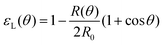 is the strain caused by fusion.36 The corresponding strain rate reads
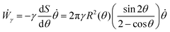
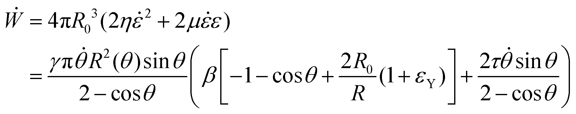
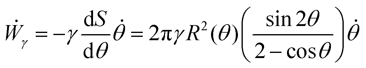
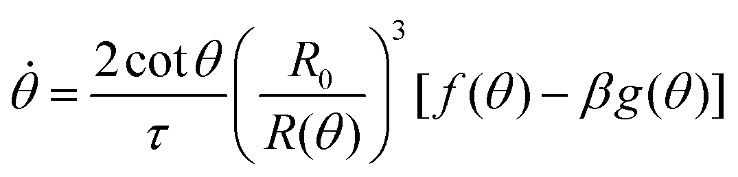
 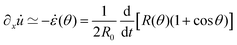 . The previous expression differs from the one used in ref. 26 and 28–31, where strain is defined using the distance between the center of a droplet in the assembly and the fusion plane (i.e. R(θ)cosθ), as opposed to the end-to-end length L(θ). Both expressions are only equivalent for small angles (i.e. θ ≪ 1). We will use the end-to-end distance definition to be consistent with previous studies on arrested coalescence,36 where the maximum strain for complete coalescence reads εL(π/2) = 1–2−2/3 ≃ 0.37. Using the previous expressions we can calculate the dynamics of θ by equating the work per unit time done by the bulk and surface forces31 (see Appendix). The equation for the dynamics of the fusion angle θ(t) reads
| |  | (1) |
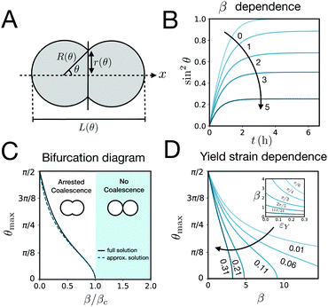
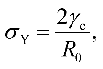
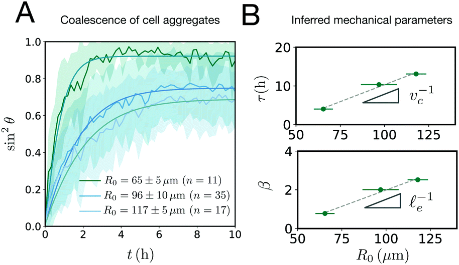
where τ = ηR0/γ is the characteristic viscocapillary time and β = μR0/γ is a dimensionless parameter characterizing the degree of fusion. The latter dimensionless number is related to the shear elastocapillary length e = R0/β. Finally, f(θ) and g(θ) are functions that depend on the angle θ (see Appendix). The viscoelastic relaxation time can be obtained as τv ≡ η/μ = τ/β = e/vc. For small angles and β = 0, eqn (1) reduces to the typical form for the sintering of viscous drops.30,31 Considering β as our bifurcation parameter, we find that for β > βc = 1/εY, elasticity overcomes surface tension and the stable state is θ = 0, i.e. no fusion (see Appendix). However, for β < βc, the system undergoes a pitchfork bifurcation whereby the state θ = 0 becomes unstable and droplets fuse (Fig. 2B and C). This critical condition β = βc is equivalent to  which means that coalescence starts when the Laplace pressure equals a yield stress σY = 2μεY. Finally, in Fig. 2D we show the dependence of the maximum fusion angle θmax on β, as a function of the yield strain εY. For the low coalescence regime, to achieve a given steady-state angle θmax, changes in εY are accompanied by large changes in β. However, in the high coalescence regime, the values of θmax are weakly dependent on εY, i.e. large changes in εY are accompanied by small changes in β (see Fig. 2D, inset). Given that our experimental data were found in the latter regime (the minimum steady state angle is ∼1 rad), for simplicity we assumed εY = 0. Image analysis was performed for each aggregate by using the software MOrgAna (see ref. 50 and Appendix). By tracking the end-to-end distance of the assembly L over time, we inferred the time evolution of the fusion angle θ (see Fig. S2, ESI† and Appendix). The study was carried out by averaging n = 63 fusion events using different aggregate sizes (see Fig. 3A). The resulting curves were numerically fitted to the solution of eqn (1) (Fig. 3A). In Fig. 3B, the inferred parameters τ and β are shown to scale linearly with the aggregate size R0, in agreement with our linear viscoelastic solid model. From the slopes of Fig. 3B, we obtain vc = 0.10 ± 0.01 μm min−1, e = 30 ± 4 μm and τv = 5.0 ± 0.8 h (n = 63 fusion events). These results were combined with nanoindentation measurements (Fig. S3, ESI†) where the Hertz model was fitted to the indentation curves (see Appendix). The average shear modulus was μ = 33 ± 4 Pa (mean ± SE, n = 25 aggregates), leading to an effective surface tension γ = 1.0 ± 0.2 mN m−1 and viscosity η = (6 ± 1) × 105 Pa s. The viscosity and elasticity values are found in the typical range,19,21,25,32 while the surface tension is found in the lower bound of typical values, similar to neural retina or embryonic chicken tissues.19
 |
| | Fig. 2 (A) Schematics of two identical droplets fusing along the ex axis. θ is the angle of fusion which is π/2 for complete coalescence and takes a value in the range (0, π/2) for arrested coalescence. R(θ) is the radius of each aggregate, r(θ) is the neck radius during the fusion process and L(θ) is the end-to-end length. (B) Time evolution of (r/R)2 = sin2θ as a function of the inverse elastocapillary number β for τ = 4 h and εY = 0.11 by solving eqn (1) (see Appendix). (C) Bifurcation diagram showing the steady state coalescence angle θmax as a function of β/βc. For β < βc the system undergoes a pitchfork bifurcation where the non-fused state loses stability in favour of the fused state. The numerical steady state solution of eqn (1) is shown as a solid line while the approximate analytical solution assuming R(θ) ≈ R0 is shown as a dashed line (see Appendix). εY = 0.11. (D) Yield strain dependence of θmax on β by solving eqn (1) numerically at steady state. Inset: β dependence on the yield strain εY for different θmax values (in radians). | |
 |
| | Fig. 3 (A) Fusion dynamics quantification showing the averaged time evolution of sin2θ, where θ is the fusion angle of the assembly (see Fig. 2). Three different aggregate sizes are shown (shaded regions denote SD around the mean experimental curve). The numerical fits (solid lines) are obtained using eqn (1). (B) The parameters τ and β scale linearly with the aggregate size as expected from the theory. From the slope the viscocapillary velocity vc and shear elastocapillary length e can be inferred (mean ± SD. Errors in the y-axis are smaller than the symbol size, n = 63 fusion events). | |
3 Agent-based simulations
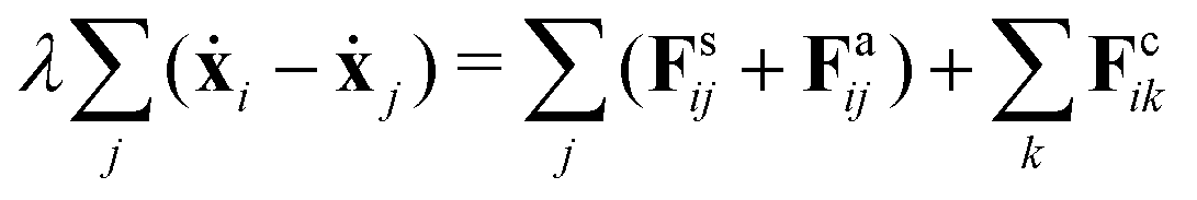
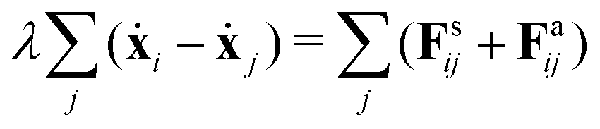
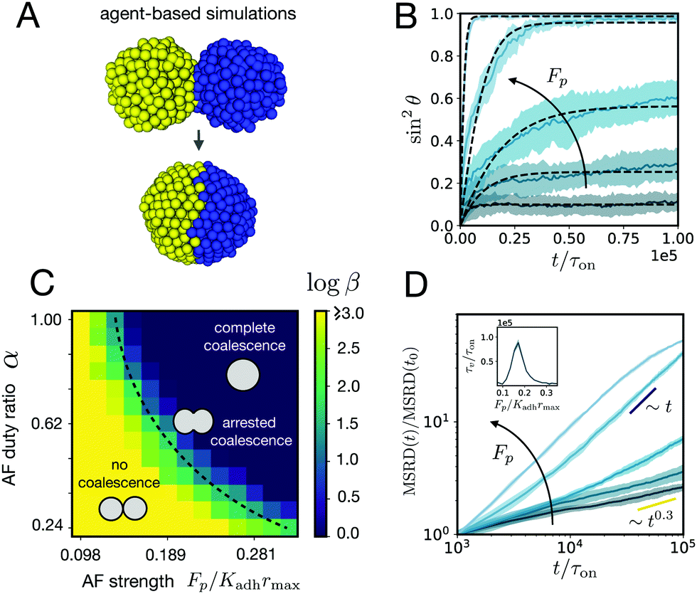
Despite the Kelvin–Voigt model providing a good fit to the experimental data, the rheology of cell aggregates is indeed much more complicated and it is unclear how cell–cell interactions give rise to the observed effective macroscopic mechanical properties. To understand this, we turned to agent-based simulations of cellular aggregates using the GPU-based software ya‖a (see Fig. 4A), which supports easy implementation of diverse cellular behaviours.51 For simplicity, we considered a minimal model taking into account passive and active interactions between cells, similarly to other agent-based models describing multicellular aggregates.31,47,52,53 The dynamics of a cell i with center at xi reads:| |  | (2) |
where j runs over the nearest neighbours, Fsij is a passive cell–cell interaction force and Faij is an active force modeling cellular contractile forces, which are known to be important in convergence-extension and cell sorting processes.54,55 Friction forces are considered to be proportional to the relative velocity of neighbouring cells with friction coefficient λ, a typical assumption used in foam and colloidal systems56,57 as well as in tissues.52,58 Cells have radius r0 and the distance between a pair of cells i and j is denoted as rij = xi − xj. The passive cell–cell interaction force consists of two parts: a repulsion harmonic force Fsij = Kr(2r0 − |rij|)![[r with combining circumflex]](https://www.rsc.org/images/entities/b_char_0072_0302.gif) ij for |rij| < 2r0 that describes excluded volume interactions and a truncated harmonic attractive force describing cell–cell adhesion for |rij| ≥ 2r0 such that Fsij = Kadh(2r0 − |rij|)Θ(rmax − |rij|), where
ij for |rij| < 2r0 that describes excluded volume interactions and a truncated harmonic attractive force describing cell–cell adhesion for |rij| ≥ 2r0 such that Fsij = Kadh(2r0 − |rij|)Θ(rmax − |rij|), where ![[r with combining circumflex]](https://www.rsc.org/images/entities/b_i_char_0072_0302.gif) ij = rij/|rij|. The active part Faij consists of cells randomly selecting a nearest neighbour and applying a constant force Faij = −Fpij if |rij| ≥ 2r0, where Fp > 0 is defined as contractile (see Appendix). We associate a lifetime with each cell–cell interaction τon and analogously, a waiting time τoff. Thus a duty ratio can be defined as α = τon/(τon + τoff). The described dynamics is similar to a shot noise process of active origin.59 Hence, cellular contractile interactions introduce force dipoles stochastically in the cell aggregate generating active fluctuations, which are known to induce cell–cell rearrangements that fluidize tissues.60–62
ij = rij/|rij|. The active part Faij consists of cells randomly selecting a nearest neighbour and applying a constant force Faij = −Fpij if |rij| ≥ 2r0, where Fp > 0 is defined as contractile (see Appendix). We associate a lifetime with each cell–cell interaction τon and analogously, a waiting time τoff. Thus a duty ratio can be defined as α = τon/(τon + τoff). The described dynamics is similar to a shot noise process of active origin.59 Hence, cellular contractile interactions introduce force dipoles stochastically in the cell aggregate generating active fluctuations, which are known to induce cell–cell rearrangements that fluidize tissues.60–62
 |
| | Fig. 4 (A) ya‖a agent-based simulations of the fusion of two cell aggregates for Fp/Kadhrmax = 0.20 and α = 1. (B) Averaged time evolution of sin2θ over time (n = 10, shaded region denotes SD around the mean simulation curve) in the simulations for different active fluctuation strengths Fp/Kadhrmax = (0.098, 0.116, 0.134, 0.171, and 0.208). Kadh/Kr = 1, r0/rmax = 0.4, λ/Kadhτon = 1, α = 1, and 500 cells per aggregate. The numerical fits (dashed lines) are obtained using eqn (1). (C) Effect of active fluctuations (AF) to the fusion of the cell aggregates. Color map of logβ in parameter space. Three distinct regions can be identified corresponding to no coalescence, arrested coalescence and complete coalescence. (D) Mean squared relative displacement of cells as a function of time for different active fluctuation strengths Fp/Kadhrmax (same values as in panel B). Cells change from a subdiffusive (∼t0.3) to a diffusive (∼t) behaviour for increasing Fp. t0/τon = 103. Inset: Viscoelastic relaxation time vs. active fluctuation strength. | |
We analyzed the fusion dynamics in the simulations by using the end-to-end length of the assembly as in the experiments and varied the active force Fp and the duty ratio α (see Fig. 4). We fitted eqn (1) to the averaged dynamics (Fig. 4B) and extracted the effective macroscopic parameters τ and β. The study revealed the presence of three main regimes depending on β (see Movies S2–S4, ESI†): (i) no coalescence (β ≳ 20), (ii) arrested coalescence (20 ≳ β ≳ 1) and (iii) complete coalescence (β ≲ 1) (Fig. 4C), which qualitatively agree with the regimes found in the continuum model (Fig. 2). The same regimes are also identified when studying the characteristic viscocapillary time τ (see Fig. S4, ESI†). These results suggest that the system undergoes a solid-to-fluid transition for increasing strength or duty ratio of the active fluctuations. To assess if the observed transition is similar to a rigidity or a jamming transition, we studied the relative mean squared displacement of cells in our simulations (Fig. 4D). We found that in regimes (i) and (ii) the behaviour was subdiffusive while the behaviour was mainly diffusive in regime (iii). In addition, we observed that the viscoelastic relaxation time τv diverges close to the transition point (see Fig. 4D, inset), which is reminiscent of a critical slowing down phenomenon observed in jammed systems.53,63,64 In order to verify if phase (i) corresponded to a jammed phase, we performed compression/relaxation cycles in parallel plate compression simulations on the aggregates (see Fig. S5 and Movies S5, S6, ESI†) and identified the presence of a yield stress in regime (i), below which the deformation was not recovered during the relaxation process, indicating a plastic behaviour of the material.65 Hence, we conclude that in our simulations, arrested coalescence is found at the vicinity of a solid-to-fluid transition, similarly to jammed systems.
4 Conclusions
Here we report the phenomenon of arrested coalescence in stem cell aggregates and present a viscoelastic theory of sintering to understand the dynamics of the process. We show that a minimal agent-based model considering cell–cell adhesion and dipolar contractile forces can account for arrested coalescence. Additionally, we find that cellular active fluctuations can control a solid-to-fluid transition. By combining simulations and continuum theory, we are able to study the dependence of different hydrodynamic quantities on cell–cell interactions. The role of cellular contractile interactions is twofold: on the one hand, they lead to a fluidization process (Fig. 4D) and, on the other hand, they create an effective surface tension γ that drives the coalescence of the cell aggregates. Although the solid-to-fluid transition is of active origin, it is different from other transitions observed in models of self-propelled particles.66,67 Instead, the transition we find resembles structural transitions driven by force dipoles during zebrafish blastoderm fludization68 or during body axis elongation.69 In particular, in the last study, tissue fluidization was shown to be driven by active tension fluctuations at cell–cell contacts in a 2D vertex model with extracellular spaces.69 Considering the timescale of our active fluctuations to be similar to tension fluctuations in cell–cell contacts (τon ∼ 10 s),69 the fusion time in our simulations corresponds to ∼10 h (see Movie S3, ESI†) consistent with the experiments. Our work adds to the previous theoretical studies suggesting an important role of active fluctuations in cellular unjamming.14,70 It is worth mentioning that despite the fact that arrested coalescence is found close to a solid-to-fluid transition in our simulations, it is unclear if this is the case in the experiments. In particular, while the experimental sin2θ curves level off at values of ∼0.5, this is not the case in simulations where we observe very slow fusion dynamics close to the transition point. This is a consequence of a divergence in the viscoelastic relaxation time of the system as shown in Fig. 4D (inset). Similar results were found in a recent study from Ongenae et al., where they considered a different model including protrusive forces and active cell motility.53 Other forms of arrested behaviour in 3D active aggregates should be further investigated, for example, including the effect of extracellular matrix elasticity. Finally, an intrinsic limitation of our particle-based simulations is the absence of cell shape changes which are known to be critical in tissue rheology.69,71–73 Further work is required to incorporate such effects, for example, by means of 3D vertex models.74
Continuum descriptions of drop coalescence have been mainly limited to purely viscous drops.28–31 This has limited the use of such theories to the determination of viscosity and surface tension, despite tissue stiffness and viscoelastic effects having important implications for tissue engineering and being known to play a major role in cancer.75,76 Here we present a simple method that when combined with a contact method such as nanoindentation or AFM, allows a fast full mechanical characterisation of 3D tissue aggregates. It is important to notice that nanoindentation measurements are done in a timescale of seconds while fusion experiments occur in a timescale of hours. This is a limitation of our method that should be taken into account when interpreting the measurements. Apart from mouse embryonic stem cells, we successfully applied our model to characterise the arrested coalescence behaviour of human stem cell aggregates (Fig. S6 and Movie S7, ESI†) and human breast epithelial cell aggregates (Fig. S7, based on data from ref. 41). Hence, our method constitutes a promising tool in the bioengineering and medical fields for the mechanical characterization of tissue spheroids. More generally, the method can also be potentially used to characterise the mechanics of inert drops in the emulsion industry. Finally, we envision that future work on the theory of sintering for viscoelastic materials will be important in the formation of biological structures in vitro using bioink units.77
Author contributions
Conceptualization: D. O. and V. T.; data curation: D. O.; formal analysis: D. O. and V. T.; funding acquisition: D. O., N. G., M. S.-M., M. E., J. S., V. T.; investigation: D. O., M. M.-R., K. A., M. S.-M., G. A.; methodology: D. O., M. M.-R., K. A., N. G.; project administration: J. S., M. E., V. T.; software: M. M.-R., N. G.; writing: D. O., M. M.-R., V. T.
Conflicts of interest
There are no conflicts to declare.
Appendix
Materials and methods
Mouse ES cell culture and 3D aggregate formation.
T/Bra::GFP mouse embryonic stem cells78 were maintained in ES-Lif (ESLIF) medium, consisting of KnockOut Dulbecco's Modified Eagle's Medium (DMEM) supplemented with 10% fetal bovine serum (FBS), 1× non-essential aminoacids (NEEA), 50 U mL−1 Pen/Strep, 1× GlutaMax, 1× sodium pyruvate, 50 μM 2-mercaptoethanol and leukemia inhibitory factor (LIF). Cells adhered to 0.1% gelatin-coated (Millipore, ES-006-B) tissue culture-treated 25 cm2 flasks (T25 flasks, Corning, 353108) in an incubator at 37 °C and 5% CO2. To form the aggregates ∼300 cells were aggregated per well in 96-well U-bottom plates (Greiner Cellstar, #650970) containing 40 μL NDiff227 media (Takara Bio, #Y40002) for 24 h prior to fusion. To ensure the state of the cells was the same in all fusion events, only the multicellular aggregates that did not express T/Bra (mesodermal marker) at 24 h were considered.
Image acquisition, feature extraction and fitting procedure.
2D images of cell aggregates in 96-well microplates were acquired using the high content imaging PerkinElmer Opera Phenix® system in non-confocal bright field mode. A 10× air objective was used with 0.3 N.A. and an exposure time of 100 ms. To capture the dynamics of the fusion process, snapshots were acquired every 10 min for a duration of 10 h. All time points were segmented using the software MOrgAna (Machine-learning based Organoid Analysis),50 a Python-based machine learning software (https://github.com/LabTrivedi/MOrgAna.git). To fit our model to the experiments, the end-to-end distance of the assembly L was obtained by fitting an ellipse to the final mask at every time frame. The fitting error due to the irregular shape of the fused assemblies was reduced by averaging over many fusion events (see Fig. S2, ESI†). Finally, using the relationship L(θ) = 2R(θ)(1 + cosθ) and considering L(0) = 4R0, the time evolution of the fusion angle θ(t) was obtained. Finally, the experimental and simulated data were fitted to the solution of eqn (1) using a non-linear least squares method. The solution of eqn (1) was obtained numerically using the Python solver odeint and the fitting was done using curve_fit, both functions from the Python package SciPy.79
Nanoindentation measurements.
The mechanical measurements were done using the Chiaro Nanoindenter (Optics11) adapted to a Leica DMi8 inverted microscope. The aggregates were transferred from the multiwell plates to μ-Slide 8 well coverslips (ibidi, #80826) coated with 0.1% gelatin and containing warm NDiff227. Indentations were done with a spherical cantilever probe of 27 ± 3 μm of radius and a stiffness of 0.025 ± 0.002 N m−1. The approach speed was 5 μm s−1 and the indentation depth was ≃6 μm (∼3% of the typical size of an aggregate). The effective elastic modulus Eeff was calculated by fitting the Hertz's model to the indentation curves and the corresponding shear modulus was obtained as μ = (Eeff/2)(1 − ν2)/(1 + ν),80 assuming a Poisson's ratio of ν = 1/2. The effective elastic modulus for each aggregate was obtained by averaging around 3–4 measurements. Finally, the average effective elastic modulus was obtained by averaging over n = 25 different aggregates.
Continuum modeling
Kelvin–Voigt model.
We consider a multicellular aggregate as a homogeneous incompressible Kelvin–Voigt material drop with effective shear viscosity η, shear modulus μ and surface tension γ. Hereinafter, we use index notation and Einstein's summation convention. The constitutive equation for the stress tensor σij reads| | | σij = 2ηij + 2μεij − Pδij | (8) |
where  is the symmetric strain tensor, P is the hydrostatic pressure and ui is the displacement field. The continuity equation readswhere vi =
 ![[u with combining dot above]](https://www.rsc.org/images/entities/i_char_0075_0307.gif) i. The latter condition is valid provided that cell proliferation is negligible in the system. Force balance in the bulk in the absence of external forces readsSimilarly, force balance on the surface readswhere H is the local mean curvature of the surface and ni is the unit normal vector to the surface. Let us now consider the fusion of two identical spherical aggregates. The total volume and area of the assembly will be denoted by V and S, respectively. The work of the viscoelastic forces per unit time Ẇ(t) reads
i. The latter condition is valid provided that cell proliferation is negligible in the system. Force balance in the bulk in the absence of external forces readsSimilarly, force balance on the surface readswhere H is the local mean curvature of the surface and ni is the unit normal vector to the surface. Let us now consider the fusion of two identical spherical aggregates. The total volume and area of the assembly will be denoted by V and S, respectively. The work of the viscoelastic forces per unit time Ẇ(t) reads| | 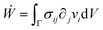 | (12) |
where Γ(t) and ∂Γ(t) denote the integration domains of the volume and surface of the assembly, respectively. Using the force balance in the bulk (eqn (2)), the divergence theorem and force balance on the surface (eqn (11)) one finds26,28–31| |  | (13) |
where the last equality on the right-hand side corresponds to the work done by the surface tension forces per unit time, which we refer as to Ẇγ. At the same time, Ẇγ can also be expressed simply as| |  | (14) |
Combining eqn (12) and (13) we find26,28–31The previous expression states that the work done by the bulk forces per unit time equals the work done by the surface forces per unit time. Following previous work,26,28–31,45,46 we model the two fusing aggregates as two spherical caps of radius R(θ) with a circular contact ‘neck’ region of radius r(θ) = R(θ)sinθ (see Fig. 2A). The volume V(θ) and surface S(θ) of two fused droplets with a fusion angle θ can be obtained by using simple geometric considerations:26| | 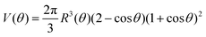 | (16) |
| | | S(θ) = 4πR2(θ)(1 + cosθ) | (17) |
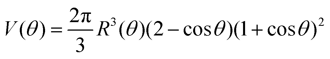
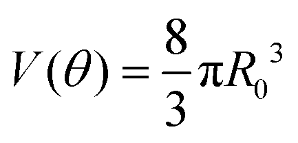
Given that ∂ivi = 0, the total volume of the assembly V will be conserved during the fusion process. Considering an initial radius of the aggregates R(0) = R0, the total volume of the assembly reads  . From the previous equation we obtain R(θ) as follows:31
| | | R(θ) = 22/3(1 + cosθ)−2/3(2 − cosθ)−1/3R0 | (18) |
The dynamics of the fusion process will be completely determined by the evolution of θ(t), with θ(0) = 0 to θ(∞) = θmax. Let us assume the axis of fusion is ex (see Fig. 2A). The end-to-end length L(θ) of the fusion assembly along this axis will be given by| | | L(θ) = 2R(θ)(1 + cosθ) | (19) |
As mentioned in the main text, our hydrodynamic model cannot capture the physics at the onset of fusion and we add a yield strain to effectively account for an elasticity threshold value for the fusion of viscoelastic solid drops.36 We consider a shifted rest length L′(0) = L(0) + δL, being δL/L′(0) ≪ 1. We approximate the strain as ∂xu ≃ −ε(θ), where ε(θ) reads| | 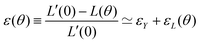 | (20) |
with εY = δL/L′(0) and εL(θ) having the following expression:36| | 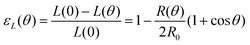 | (21) |
We approximate the corresponding strain rate as ∂xv ≃ −(θ), where (θ) reads| | 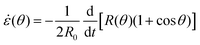 | (22) |
The previous expression differs from the usual one, used in ref. 26 and 28–31, which is based on a definition of strain as changes in the center-to-center length of the fusion assembly (as opposed to end-to-end as in eqn (21)). Using eqn (20) and the fact that the system is incompressible, we obtain an approximation for the strain tensor:| |  | (23) |
Using the previous simplified expressions we can calculate the work per unit time done by the bulk and surface forces:| | 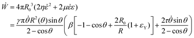 | (24) |
| |  | (25) |
where τ = ηR0/γ is the characteristic viscocapillary time and β = μR0/γ is a dimensionless parameter quantifying the degree of fusion. The shear elastocapillary length reads e ≡ γ/μ = R0/β. Using eqn (15) we find an equation for the dynamics of the fusion angle θ(t):| | 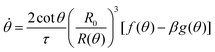 | (26) |
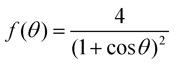
where f(θ), g(θ) read| | 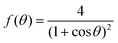 | (27) |
| | 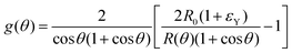 | (28) |
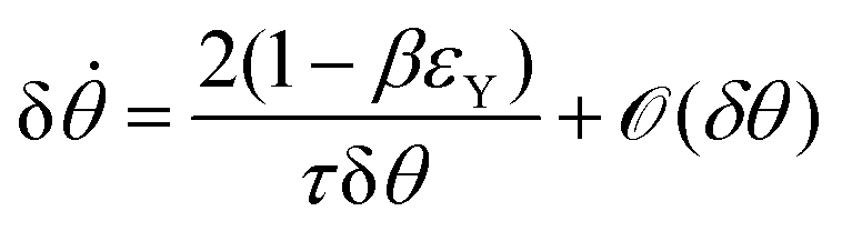
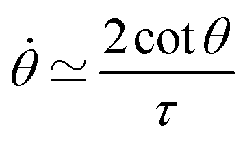
Notice that from eqn (26) the viscocapillary time τ is a factor of 4 larger than the usual definition.26,28–31 This is a consequence of our choice of strain in eqn (21) which is twice as small as the usual one. For small angles and β = 0, eqn (26) reduces to the typical form for the sintering of viscous drops30,31 (see eqn (34) in Connection to previous studies of viscous drops). Let us study the stability of the system around θ = 0. The dynamics of a perturbation δθ ≪ 1 reads| | 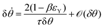 | (29) |
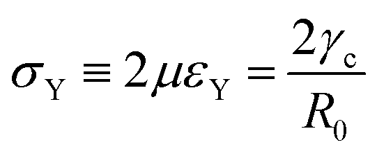
Hence for β < βc = 1/εY, the non-fused state θ = 0 loses stability. Notice that in the absence of yield strain (i.e. εY = 0) the non-fused state is always unstable and hence, two drops in contact will always fuse. The critical condition is equivalent to| | 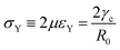 | (30) |
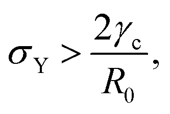
which means that the yield point corresponds to when the yield stress σY equals the Laplace pressure. When the Laplace pressure is larger than the yield stress of the material  fusion starts. Considering R(θ) ≈ R0, we can obtain an analytical expression for θmax as a function of β by solving eqn (26) at steady state:
| | 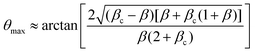 | (31) |
As expected, the angle of arrested coalescence is independent of the viscocapillary time τ and only depends on β. Close to the critical point β = βc, the arrested fusion angle reads θmax ∼ ε1/2, where ε ≡ (βc − β)/βc is a small parameter that characterizes the distance to the critical point. Hence the system is completely determined by three parameters: τ, β and εY.
Connection to previous studies of viscous drops.
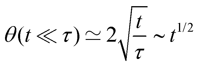
Here we connect our results to previous classical results in the literature of the sintering of purely viscous droplets. For β = εY = 0 and small angles (θ ≪ 1), eqn (26) can be approximated to the well known form:| |  | (32) |
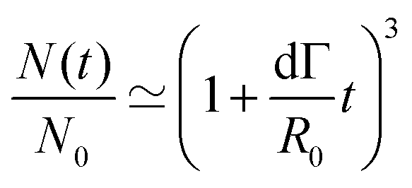
This expression is equivalent to the typical form with the only difference being that the viscocapillary time is a factor 4 larger than the usual definition.77 By solving this equation we find that sin2θ(t) follows77| | | sin2θ(t) ≃ 1 − e−4t/τ | (33) |
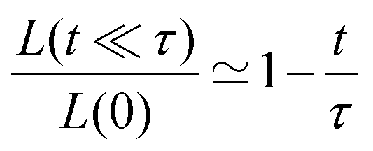
A well known scaling relation for the evolution of the angle for t ≪ τ is| | 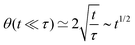 | (34) |
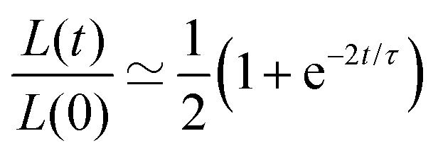
Another useful expression is the time dependence of the relative shrinkage of the assembly assuming R(t) ≃ R0:| |  | (35) |
the last expression is related to the evolution of the aspect ratio.83,84 For short-timescales (t ≪ τ) the previous expression reduces to| | 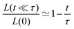 | (36) |
Agent-based simulations
All agent-based simulations were programmed in CUDA C++ using the ya||a modelling framework (https://github.com/germannp/yalla). The neighbour search method used to determine the pairwise interactions is a modified version of the overlapping spheres method,51,85 where the Gabriel method is applied to a preliminary set of nearest neighbours in order to eliminate neighbour interactions that are being blocked by a third, nearer neighbour.86,87 The equations of motion (eqn (2)) were solved using the two-step Heun method.51
Active cell–cell interaction dynamics.
At every time step, the active cell–cell dynamics is simulated in the following way: for a set of N cells we define N effective ‘protrusions’, each protrusion Pi being produced by each cell i. The protrusion Pi always has one end at xi and can be connected to another cell j at xj. At any time point, Pi can be “on”, that is connecting cell i to cell j and applying a force of magnitude Fp (see main text), or it can be “off”, that is not connected to a cell j and thus not applying any force. The probabilities that Pi are switched “on” or “off” during the time step Δt are given by 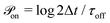 and
and 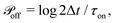 respectively. At every time step, for each protrusion Pi, it is stochastically determined whether Pi should be updated given the probabilities
  (if Pi is currently off) or
  (if Pi is currently on). If that is the case and the current state is “on”, Pi is switched off. Alternatively, if the current state is off, a random cell xj is chosen such that it is found at a distance from xi smaller than 2r0, and Pi is then connected to xj at the other end.
Fusion and parallel plate compression simulations.
For the simulation of fusion events, two separated spherical aggregates are created by randomly generating 3D points within a sphere. Next, we let the system evolve for a short transient of time to make sure the two aggregates have reached its equilibrium configuration prior to the start of the simulation. To start the fusion process we move the aggregates closer so that they contact each other. Finally, to simulate the process of parallel plate compression we defined the position of the upper/lower plate zk, k = 1, 2 as the position of the uppermost/lowermost cell over time along the z-axis. A cell i in the aggregate will experience a force Fcik from plate k defined as| | 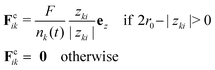 | (37) |
where zki = zk − zi is the distance between plate k and a cell i along the z-axis,  is the number of cells that fulfil the condition 2r0 − |zki| > 0 (i.e. interact with plate k) at time t, and F is the total external force applied to each plate. The extended dynamics of each cell i reads
| |  | (38) |
The initial setup consists of a single spherical aggregate of cells and two plates positioned on opposite sides of the aggregate along the z-axis. At the start of the simulation and during a certain time period, an external force of magnitude F is applied in each plate in order to compress the aggregate. After that period, the plates are removed so that relaxation can take place (see Movies S5 and S6, ESI†).
Acknowledgements
This work was conceived during the COVID-19 pandemic lockdown. We would like to thank all the healthcare professionals who fought against the disease. We thank the Mesoscopic Imaging Facility (EMBL Barcelona) for assistance with imaging and the Tissue Engineering Unit (CRG). We also thank J. Casademunt, X. Diego, M. Merkel, G. Torregrosa and all the members of the Trivedi group for illuminating discussions. D. O. acknowledges funding from Juan de la Cierva Incorporación with Project no. IJC2018-035298-I, from the Spanish Ministry of Science, Innovation and Universities (MCIU/AEI) and N. G. acknowledges the Human Frontier Science Program (HFSP) for number LT000227/2018-L. Finally, M. S.-M. is supported by the Daiichi Sankyo Foundation of Life Science and Japan Society for the Promotion of Science (JSPS) Overseas Research Fellowships. All authors were supported by the European Molecular Biology Laboratory (EMBL).
Notes and references
- C.-P. Heisenberg and Y. Bellache, Cell, 2013, 153, 948–962 CrossRef CAS PubMed.
-
H. Hamada, Seminars in cell & developmental biology, 2015, pp. 88–91 Search PubMed.
- B. P. Teague, P. Guye and R. Weiss, Cold Spring Harbor Perspect. Biol., 2016, 8, a023929 CrossRef PubMed.
- N. Gritti, D. Oriola and V. Trivedi, Dev. Biol., 2021, 474, 48–61 CrossRef CAS PubMed.
- E. Garreta, R. D. Kamm, S. M. C. de Sousa Lopes, M. A. Lancaster, R. Weiss, X. Trepat, I. Hyun and N. Montserrat, Nat. Mater., 2020, 1–11 Search PubMed.
- T. Wyatt, B. Baum and G. Charras, Curr. Opin. Cell Biol., 2016, 38, 68–73 CrossRef CAS PubMed.
- R. Clément, B. Dehapiot, C. Collinet, T. Lecuit and P.-F. Lenne, Curr. Biol., 2017, 27, 3132–3142 CrossRef PubMed.
- E.-M. Schötz, R. D. Burdine, F. Jülicher, M. S. Steinberg, C.-P. Heisenberg and R. A. Foty, HFSP J., 2008, 2, 42–56 CrossRef PubMed.
- M. Yu, A. Mahtabfar, P. Beelen, Y. Demiryurek, D. I. Shreiber, J. D. Zahn, R. A. Foty, L. Liu and H. Lin, Biophys. J., 2018, 114, 2703–2716 CrossRef CAS PubMed.
- R. Gordon, N. S. Goel, M. S. Steinberg and L. L. Wiseman, J. Theor. Biol., 1972, 37, 43–73 CrossRef CAS PubMed.
- M. S. Steinberg and M. Takeichi, Proc. Natl. Acad. Sci. U. S. A., 1994, 91, 206–209 CrossRef CAS PubMed.
- K. Heintzelman, H. Phillips and G. Davis, Development, 1978, 47, 1–15 CrossRef CAS.
- R. A. Foty, G. Forgacs, C. M. Pfleger and M. S. Steinberg, Phys. Rev. Lett., 1994, 72, 2298 CrossRef PubMed.
- A. Mongera, P. Rowghanian, H. J. Gustafson, E. Shelton, D. A. Kealhofer, E. K. Carn, F. Serwane, A. A. Lucio, J. Giammona and O. Campàs, Nature, 2018, 561, 401–405 CrossRef CAS PubMed.
- O. Luu, R. David, H. Ninomiya and R. Winklbauer, Proc. Natl. Acad. Sci. U. S. A., 2011, 108, 4000–4005 CrossRef CAS PubMed.
- K. Sugimura, P.-F. Lenne and F. Graner, Development, 2016, 143, 186–196 CrossRef CAS PubMed.
- O. Campàs, Semin. Cell Dev. Biol., 2016, 119–130 CrossRef PubMed.
- R. A. Foty, C. M. Pfleger, G. Forgacs and M. S. Steinberg, Development, 1996, 122, 1611–1620 CrossRef CAS PubMed.
- G. Forgacs, R. A. Foty, Y. Shafrir and M. S. Steinberg, Biophys. J., 1998, 74, 2227–2234 CrossRef CAS PubMed.
- R. David, H. Ninomiya, R. Winklbauer and A. W. Neumann, Colloids Surf., B, 2009, 72, 236–240 CrossRef CAS PubMed.
- K. Guevorkian, M.-J. Colbert, M. Durth, S. Dufour and F. Brochard-Wyart, Phys. Rev. Lett., 2010, 104, 218101 CrossRef PubMed.
- O. Campàs, T. Mammoto, S. Hasso, R. A. Sperling, D. O'connell, A. G. Bischof, R. Maas, D. A. Weitz, L. Mahadevan and D. E. Ingber, Nat. Methods, 2014, 11, 183 CrossRef PubMed.
- F. Serwane, A. Mongera, P. Rowghanian, D. A. Kealhofer, A. A. Lucio, Z. M. Hockenbery and O. Campàs, Nat. Methods, 2017, 14, 181 CrossRef CAS PubMed.
- I. Bonnet, P. Marcq, F. Bosveld, L. Fetler, Y. Bellache and F. Graner, J. R. Soc., Interface, 2012, 9, 2614–2623 CrossRef PubMed.
- K. Jakab, B. Damon, F. Marga, O. Doaga, V. Mironov, I. Kosztin, R. Markwald and G. Forgacs, Dev. Dyn., 2008, 237, 2438–2449 CrossRef PubMed.
- G. Dechristé, J. Fehrenbach, E. Griseti, V. Lobjois and C. Poignard, J. Theor. Biol., 2018, 454, 102–109 CrossRef PubMed.
- R. David, O. Luu, E. W. Damm, J. W. Wen, M. Nagel and R. Winklbauer, Development, 2014, 141, 3672–3682 CrossRef CAS PubMed.
- J. Frenkel, J. Phys., 1945, 9, 385 Search PubMed.
- O. Pokluda, C. T. Bellehumeur and J. Vlachopoulos, AIChE J., 1997, 43, 3253–3256 CrossRef CAS.
- M. K. Bellehumeur, T. Céline and J. Vlachopoulos, Rheol. Acta, 1998, 37, 270–278 CrossRef.
- E. Flenner, L. Janosi, B. Barz, A. Neagu, G. Forgacs and I. Kosztin, Phys. Rev. E: Stat., Nonlinear, Soft Matter Phys., 2012, 85, 031907 CrossRef PubMed.
- T. V. Stirbat, A. Mgharbel, S. Bodennec, K. Ferri, H. C. Mertani, J.-P. Rieu and H. Delanoë-Ayari, PLoS One, 2013, 8, e52554 CrossRef CAS PubMed.
- L. Zhao, Y. Liu, Y. Liu, M. Zhang and X. Zhang, Anal. Chem., 2020, 92, 7638–7645 CrossRef CAS PubMed.
- P. Dahiya, M. Caggioni and P. T. Spicer, Philos. Trans. R. Soc., A, 2016, 374, 20150132 CrossRef PubMed.
-
P. Dahiya, Arrested Coalescence in Food Emulsions, 2017 Search PubMed.
- A. B. Pawar, M. Caggioni, R. W. Hartel and P. T. Spicer, Faraday Discuss., 2012, 158, 341–350 RSC.
- Z. Xie, C. J. Burke, B. Mbanga, P. T. Spicer and T. J. Atherton, Soft Matter, 2019, 15, 9587–9596 RSC.
- V. Muguet, M. Seiller, G. Barratt, O. Ozer, J. Marty and J. Grossiord, J. Controlled Release, 2001, 70, 37–49 CrossRef CAS PubMed.
- R. S. Garabedian and J. J. Helble, J. Colloid Interface Sci., 2001, 234, 248–260 CrossRef CAS PubMed.
- A.-C. Tsai, Y. Liu, X. Yuan and T. Ma, Tissue Eng., Part A, 2015, 21, 1705–1719 CrossRef CAS PubMed.
- S. Grosser, J. Lippoldt, L. Oswald, M. Merkel, D. M. Sussman, F. Renner, P. Gottheil, E. W. Morawetz, T. Fuhs, X. Xie, S. Pawlizak, A. W. Fritsch, B. Wolf, L.-C. Horn, S. Briest, B. Aktas, M. L. Manning and J. A. Käs, Phys. Rev. X, 2021, 11, 011033 CAS.
- D. Hu, S. Phonekeo, E. Altshuler and F. Brochard-Wyart, Eur. Phys. J.: Spec. Top., 2016, 225, 629–649 Search PubMed.
- W. Pönisch, K. B. Eckenrode, K. Alzurqa, H. Nasrollahi, C. Weber, V. Zaburdaev and N. Biais, Sci. Rep., 2018, 8, 1–10 Search PubMed.
- J. Eshelby, Trans. AIME, 1949, 185, 806 Search PubMed.
- S. Aid, A. Eddhahak, Z. Ortega, D. Froelich and A. Tcharkhtchi, J. Mater. Sci., 2017, 52, 11725–11736 CrossRef CAS.
-
D. D. Joseph, Fluid dynamics of viscoelastic liquids, Springer Science & Business Media, 2013, vol. 84 Search PubMed.
- W. Pönisch, C. A. Weber, G. Juckeland, N. Biais and V. Zaburdaev, New J. Phys., 2017, 19, 015003 CrossRef PubMed.
- H.-S. Kuan, W. Pönisch, F. Jülicher and V. Zaburdaev, Phys. Rev. Lett., 2021, 126, 018102 CrossRef CAS PubMed.
- J. Bico, É. Reyssat and B. Roman, Annu. Rev. Fluid Mech., 2018, 50, 629–659 CrossRef.
- N. Gritti, J. L. Lim, K. Anlaş, M. Pandya, G. Aalderink, G. Martínez-Ara and V. Trivedi, Development, 2021, 148, dev199611 CrossRef CAS PubMed.
- P. Germann, M. Marin-Riera and J. Sharpe, Cell Syst., 2019, 8, 261–266 CrossRef CAS PubMed.
- P. Van Liedekerke, M. Palm, N. Jagiella and D. Drasdo, Comput. Particle Mech., 2015, 2, 401–444 CrossRef.
- S. Ongenae, M. Cuvelier, J. Vangheel, H. Ramon and B. Smeets, Front. Phys., 2021, 9, 1–8 Search PubMed.
- E. Palsson and H. G. Othmer, Proc. Natl. Acad. Sci. U. S. A., 2000, 97, 10448–10453 CrossRef CAS PubMed.
- J. M. Belmonte, M. H. Swat and J. A. Glazier, PLoS Comput. Biol., 2016, 12, e1004952 CrossRef PubMed.
- D. J. Durian, Phys. Rev. Lett., 1995, 75, 4780 CrossRef CAS PubMed.
- B. P. Tighe, Phys. Rev. Lett., 2011, 107, 158303 CrossRef PubMed.
- Y. Mao, A. L. Tournier, A. Hoppe, L. Kester, B. J. Thompson and N. Tapon, EMBO J., 2013, 32, 2790–2803 CrossRef CAS PubMed.
- E. Ben-Isaac, Y.-K. Park, G. Popescu, F. L. H. Brown, N. S. Gov and Y. Shokef, Phys. Rev. Lett., 2011, 106, 238103 CrossRef PubMed.
- J. Ranft, M. Basan, J. Elgeti, J.-F. Joanny, J. Prost and F. Jülicher, Proc. Natl. Acad. Sci. U. S. A., 2010, 107, 20863–20868 CrossRef CAS PubMed.
- D. Oriola, R. Alert and J. Casademunt, Phys. Rev. Lett., 2017, 118, 088002 CrossRef PubMed.
- N. I. Petridou, S. Grigolon, G. Salbreux, E. Hannezo and C.-P. Heisenberg, Nat. Cell Biol., 2019, 21, 169–178 CrossRef CAS PubMed.
- T. Hatano, Phys. Rev. E: Stat., Nonlinear, Soft Matter Phys., 2009, 79, 050301(R) CrossRef PubMed.
- K. Saitoh, T. Hatano, A. Ikeda and B. P. Tighe, Phys. Rev. Lett., 2020, 124, 118001 CrossRef CAS PubMed.
- N. J. Balmforth, I. A. Frigaard and G. Ovarlez, Annu. Rev. Fluid Mech., 2014, 46, 121–146 CrossRef.
- S. Henkes, Y. Fily and M. C. Marchetti, Phys. Rev. E: Stat., Nonlinear, Soft Matter Phys., 2011, 84, 040301(R) CrossRef PubMed.
- D. Bi, X. Yang, M. C. Marchetti and M. L. Manning, Phys. Rev. X, 2016, 6, 021011 Search PubMed.
- N. I. Petridou, B. Corominas-Murtra, C.-P. Heisenberg and E. Hannezo, Cell, 2021, 184, 1914–1928 CrossRef CAS PubMed.
- S. Kim, M. Pochitaloff, G. A. Stooke-Vaughan and O. Campàs, Nat. Phys., 2021, 1–8 Search PubMed.
- P.-F. Lenne and V. Trivedi, Nat. Commun., 2022, 13, 1–14 Search PubMed.
- M. L. Manning, R. A. Foty, M. S. Steinberg and E.-M. Schoetz, Proc. Natl. Acad. Sci. U. S. A., 2010, 107, 12517–12522 CrossRef CAS PubMed.
- D. Bi, J. Lopez, J. M. Schwarz and M. L. Manning, Nat. Phys., 2015, 11, 1074–1079 Search PubMed.
- M. Merkel and M. L. Manning, New J. Phys., 2018, 20, 022002 CrossRef.
- S. Okuda, Y. Inoue and T. Adachi, Biophys. Physicobiol., 2015, 12, 13–20 CrossRef CAS PubMed.
- O. Chaudhuri, J. Cooper-White, P. A. Janmey, D. J. Mooney and V. B. Shenoy, Nature, 2020, 584, 535–546 CrossRef CAS PubMed.
- C. F. Guimarães, L. Gasperini, A. P. Marques and R. L. Reis, Nat. Rev. Mater., 2020, 1–20 Search PubMed.
- I. Kosztin, G. Vunjak-Novakovic and G. Forgacs, Rev. Mod. Phys., 2012, 84, 1791 CrossRef.
- H. J. Fehling, G. Lacaud, A. Kubo, M. Kennedy, S. Robertson, G. Keller and V. Kouskoff, Development, 2003, 130, 4217–4227 CrossRef CAS PubMed.
- P. Virtanen, R. Gommers, T. E. Oliphant, M. Haberland, T. Reddy, D. Cournapeau, E. Burovski, P. Peterson, W. Weckesser, J. Bright, S. J. van der Walt, M. Brett, J. Wilson, K. J. Millman, N. Mayorov, A. R. J. Nelson, E. Jones, R. Kern, E. Larson, C. J. Carey, İ. Polat, Y. Feng, E. W. Moore, J. VanderPlas, D. Laxalde, J. Perktold, R. Cimrman, I. Henriksen, E. A. Quintero, C. R. Harris, A. M. Archibald, A. H. Ribeiro, F. Pedregosa, P. van Mulbregt and SciPy 1.0 Contributors, Nat. Methods, 2020, 17, 261–272 CrossRef CAS PubMed.
- J. Field and M. Swain, J. Mater. Res., 1993, 8, 297–306 CrossRef CAS.
- A. D. Conger and M. C. Ziskin, Cancer Res., 1983, 43, 556–560 CAS.
- J. A. Engelberg, G. E. Ropella and C. A. Hunt, BMC Syst. Biol., 2008, 2, 110 CrossRef PubMed.
- E.-M. Schoetz, M. Lanio, J. A. Talbot and M. L. Manning, J. R. Soc., Interface, 2013, 10, 20130726 CrossRef PubMed.
- C. P. Brangwynne, T. J. Mitchison and A. A. Hyman, Proc. Natl. Acad. Sci. U. S. A., 2011, 108, 4334–4339 CrossRef CAS PubMed.
- J. M. Osborne, A. G. Fletcher, J. M. Pitt-Francis, P. K. Maini and D. J. Gavaghan, PLoS Comput. Biol., 2017, 13, e1005387 CrossRef PubMed.
- M. Marin-Riera, M. Brun-Usan, R. Zimm, T. Välikangas and I. Salazar-Ciudad, Bioinformatics, 2015, 32, 219–225 Search PubMed.
- J. Delile, M. Herrmann, N. Peyriéras and R. Doursat, Nat. Commun., 2017, 8, 13929 CrossRef CAS PubMed.
|
| This journal is © The Royal Society of Chemistry 2022 |
Click here to see how this site uses Cookies. View our privacy policy here. 
 Open Access Article
 This Open Access Article is licensed under a
  *a,
Miquel
Marin-Riera
a,
Kerim
Anlaş
a,
Nicola
Gritti
a,
Marina
Sanaki-Matsumiya
a,
Germaine
Aalderink
a,
Miki
Ebisuya
a,
James
Sharpe
ab and
Vikas
Trivedi
*ac
*a,
Miquel
Marin-Riera
a,
Kerim
Anlaş
a,
Nicola
Gritti
a,
Marina
Sanaki-Matsumiya
a,
Germaine
Aalderink
a,
Miki
Ebisuya
a,
James
Sharpe
ab and
Vikas
Trivedi
*ac

 is the symmetric strain tensor, P is the hydrostatic pressure and u is the displacement field. Given that cell proliferation is negligible on the timescale of fusion, we approximate the continuity equation as ∇·
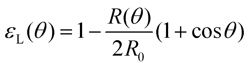 is the strain caused by fusion.36 The corresponding strain rate reads
  . The previous expression differs from the one used in ref. 26 and 28–31, where strain is defined using the distance between the center of a droplet in the assembly and the fusion plane (i.e. R(θ)
 which means that coalescence starts when the Laplace pressure equals a yield stress σY = 2μεY. Finally, in Fig. 2D we show the dependence of the maximum fusion angle θmax on β, as a function of the yield strain εY. For the low coalescence regime, to achieve a given steady-state angle θmax, changes in εY are accompanied by large changes in β. However, in the high coalescence regime, the values of θmax are weakly dependent on εY, i.e. large changes in εY are accompanied by small changes in β (see Fig. 2D, inset). Given that our experimental data were found in the latter regime (the minimum steady state angle is ∼1 rad), for simplicity we assumed εY = 0. Image analysis was performed for each aggregate by using the software MOrgAna (see ref. 50 and Appendix). By tracking the end-to-end distance of the assembly L over time, we inferred the time evolution of the fusion angle θ (see Fig. S2, ESI† and Appendix). The study was carried out by averaging n = 63 fusion events using different aggregate sizes (see Fig. 3A). The resulting curves were numerically fitted to the solution of eqn (1) (Fig. 3A). In Fig. 3B, the inferred parameters τ and β are shown to scale linearly with the aggregate size R0, in agreement with our linear viscoelastic solid model. From the slopes of Fig. 3B, we obtain vc = 0.10 ± 0.01 μm min−1,
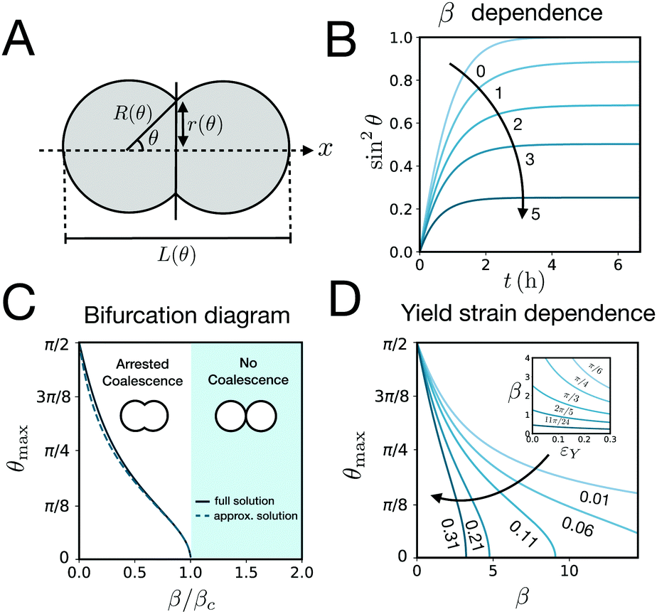
![[V with combining dot above]](https://www.rsc.org/images/entities/i_char_0056_0307.gif) = ΓVc
= ΓVc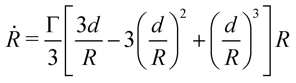
 is the symmetric strain tensor, P is the hydrostatic pressure and ui is the displacement field. The continuity equation reads

 . From the previous equation we obtain R(θ) as follows:31
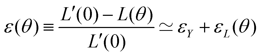


 fusion starts. Considering R(θ) ≈ R0, we can obtain an analytical expression for θmax as a function of β by solving eqn (26) at steady state:
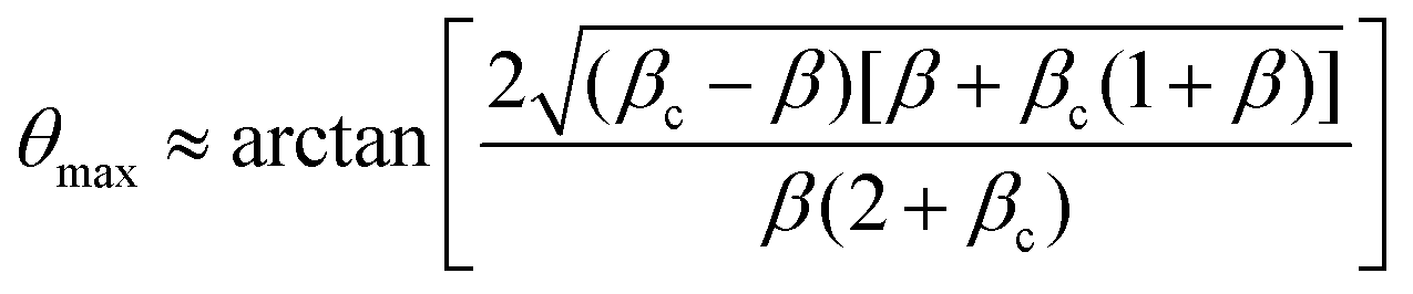
 and
and  respectively. At every time step, for each protrusion Pi, it is stochastically determined whether Pi should be updated given the probabilities
  (if Pi is currently off) or
  (if Pi is currently on). If that is the case and the current state is “on”, Pi is switched off. Alternatively, if the current state is off, a random cell xj is chosen such that it is found at a distance from xi smaller than 2r0, and Pi is then connected to xj at the other end.

 is the number of cells that fulfil the condition 2r0 − |zki| > 0 (i.e. interact with plate k) at time t, and F is the total external force applied to each plate. The extended dynamics of each cell i reads