Using small angle scattering to understand low molecular weight gels

Abstract

The material properties of a gel are determined by the underpinning network that immobilises the solvent. When gels are formed by the self-assembly of small molecules into a so-called low molecular weight gel, the network is the result of the molecules forming one-dimensional objects such as fibres or nanotubes which entangle or otherwise cross-link to form a three-dimensional network. Characterising the one-dimensional objects and the network is difficult. Many conventional techniques rely on drying to probe the network, which often leads to artefacts. An effective tool to probe the gel in the solvated state is small angle scattering. Both small angle X-ray scattering (SAXS) and small angle neutron scattering (SANS) can be used. Here, we discuss these approaches and provide a tutorial review to describe how these approaches work, what opportunities there are and how the data treatment should be approached. We aim to show the power of this approach and provide enabling information to make them accessible to the non-specialist.

---

Introduction

Gels are interesting materials, which behave as solids despite being mainly composed of a liquid. The liquid is immobilised by a network. This network can be formed by cross-linked polymers, entangled polymers, attractive colloidal particles, or formed by the self-assembly of small molecules. The latter set are called low molecular weight gels or supramolecular gels where the small molecules assemble into typically long one-dimensional structures that form a network by either entangling physically or branching to form junctions.^1–3 Low molecular weight gels are interesting both commercially and academically⁴ and have been used in a wide range of applications⁵ including tissue engineering and drug delivery,⁶ sensing,⁷ and optoelectronics.^8,9

To understand fully such low molecular weight gels requires that we can characterise the self-assembly of the gelators across all length scales (Fig. 1). The primary one-dimensional structures underpinning the gels are formed by the self-assembly on the molecular level. These primary structures then entangle, branch, laterally associate or otherwise interact to form a network (on the μm scale). On a longer length scale (on the 100 s μm scale), the properties of the gels are controlled by how these one-dimensional structures and cross-links are distributed in space. Different techniques are clearly suitable for probing the different length scales.^10–12 The local self-assembly can be determined to some degree using techniques such as spectroscopy (e.g., infra-red, UV-Vis, fluorescence, Raman, circular dichroism, nuclear magnetic resonance). Whilst important, this often does not provide information on the self-assembled structures that are formed, the cross-links and their distribution in space; these are what determine the material properties of the gels and are usually what is really of interest.

Fig. 1 Cartoon (not to scale) of the self-assembly across length scales leading to gelation.

To probe the self-assembled structure, different approaches can be taken. It is common to use a range of microscopy techniques to image the underlying structures including electron microscopy (including (cryo)-TEM, SEM),¹³ AFM¹⁴ and confocal microscopy, as well as super-resolution microscopy.^15,16 These can be extremely informative, but there are limitations. Generally, each image in these microscopy techniques covers a very small area of the sample and the data takes a relatively long time to collect. Therefore, collecting enough data to provide an averaged representation is typically not feasible, especially for a large number of samples.¹⁷ Techniques that require drying of the sample can also lead to changes in the structures present resulting in artefacts.¹⁸ The mechanical properties of the gels can be determined using techniques such as rheology, nanoindentation and compression testing.¹⁹ Whilst useful, it is extremely difficult to deconvolute differences in the data with the underlying network because a wide range of variables such as interactions at the molecular level to network density and long range (mm scale) alignment will influence the mechanical properties.

Hence, there is a real need for techniques that can be used to determine the primary structures present, how they interact and form cross-links, and the network formed on the bulk, as-formed gels. Small angle scattering approaches such as small angle X-ray scattering (SAXS) and small angle neutron scattering (SANS) are extremely powerful.^20–24 The length scales that can be probed by SAXS and SANS are on the range of 1–100 nm, and longer length scales can be accessed using ultra-small angle scattering.²⁵ These techniques can be used on bulk samples without the need for drying and provide an average of the structures present in the sample.

Our aim here in this review is to show how one can use these techniques to understand low molecular weight gels. We do not intend to provide a detailed description as to how the techniques work, or the underlying physics, but rather a user manual as to how to best collect data and then how to treat the data in different ways to best understand the systems. There is a large amount of in-depth literature covering small angle scattering theory if desired by the reader.^26–28 We also do not intend to cite every paper in the area, but rather use a sub-set of the literature to best explain how to use these techniques most effectively.

Introduction to the basic theory of small angle scattering

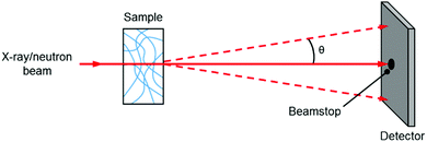
A small angle scattering experiment is one where collimated radiation is deflected through small angles (defined as 0.1–10 degrees) due to its interaction with a structure larger than the wavelength of the radiation, with objects measured falling typically into the 1–100 nm size range. In this section, we will discuss the most common experiments on gels which are small angle X-ray scattering and small angle neutron scattering.

In a typical experiment, an X-ray or neutron beam is fired at a sample (Fig. 2) and whilst most of the beam is transmitted through the sample without interaction (and is blocked from hitting the detector by a beamstop), a small proportion of the radiation is elastically scattered and impinges on (typically) a 2D detector. The angle of scattering, θ, is inversely related to the size of the object from which scattering occurs, where larger objects scatter to smaller angles.

Fig. 2 Basic cartoon schematic of a small angle scattering experiment.

SAXS experiments can be done on in-house instrumentation, where traditionally X-rays were generated by accelerated electrons striking a metal (usually copper) anode, followed by focusing through X-ray optics to reach the sample as a collimated, monochromatic beam. More modern instruments employ a liquid metal jet anode, which is continuously regenerated meaning that the limitation on X-ray flux which was imposed by the degradation of a solid anode is no longer a consideration and much higher photon fluxes can be reached, drastically reducing experimental time. However for many experiments, synchrotron radiation remains the gold standard. Here, electrons are accelerated to near relativistic speeds around a ring, giving out radiation as they do so; this radiation can be targeted to different end stations, including (but very much not limited to) SAXS, and provides users with extremely high flux meaning experiments can be carried out in air and over extremely short timescales, which opens up the possibility of exciting sample environments, some of which will be discussed later.

SANS experiments can be carried out at specialised nuclear research reactors, optimised for the generation of neutrons for scattering experiments, or at a spallation source, where neutrons are generated by first the acceleration of protons in a particle accelerator (which can be a linear accelerator (LINAC) or a LINAC combined with a synchrotron). These protons then strike a tungsten or tantalum source which generates the neutrons, which are then slowed to the energies needed for a SANS experiment using moderators of liquid hydrogen or helium.

The sample is placed in a container which is suitably transparent to the radiation in question. For static SAXS experiments, this is typically a borosilicate glass or quartz thin walled cuvette (wall thickness ∼0.01 mm). However it is also possible to undertake SAXS experiments under flow either in a flow-through cell or specially designed microfluidic device to allow changes in structure under, for example, mixing to be followed. Temperature control can be implemented on many sample holders, and there is also the possibility of coupling additional techniques such as rheology (see later) and novel sample environments such as acoustic levitation. For SANS experiments, samples are usually loaded into quartz cells. The cells come in different designs (such as cuvettes and banjo cells) with different path lengths. The cells generally have wall thicknesses of ∼1 mm.

When X-rays or neutrons are scattered by a sample, the scattering intensity (I(Q)) is measured as a function of the scattering vector, Q. Q is related to the scattering angle by eqn (1) and thus can be seen to give a size range of the scattering experiment which is agnostic to the instrument or source.

The Q range of a particular experiment is usually determined by the configuration of the instrument used, typically by the length from the sample to the detector. The longer this length, the smaller the angle which can be probed, and thus larger structures can be measured. A typical in-house instrument might cover a Q range from 0.0025 to 3 Å⁻¹, allowing measurements in real space of objects 2500 Å and 2.1 Å, whereas synchrotron beamlines can reach Q as low as 0.0011 Å⁻¹, meaning larger structures (up to 5700 Å) can be resolved.

The scattering intensity, I(Q), results from the molecular weight (M) (or size) of the scattering object, and the concentration (c) of scattering objects and is related to the difference in the scattering length density (SLD) between the object and its solvent as shown in eqn (2). However, it should be noted that certain parameters such as molecular weight or the volume of the particle require the intensity to be measured on an absolute intensity scale. During the scattering experiment, some of the X-ray photons will be transmitted through the sample, and some will be scattered; the intensity of the scattered photons therefore needs to be normalised against the intensity of the transmitted photons, which requires knowledge of the incident flux of photons, the number of photons transmitted, and the thickness of the samples. Once these are known, the data can then be plotted on an absolute scale in cm⁻¹. It can be seen from eqn (2) that I(Q) also contains information about the form factor, F(Q), which details the size and shape of the object as well as the structure factor, S(Q), which provides a measure of intraparticle interactions. For dilute, non-interacting objects, the structure factor scattering can be said to be S(Q) = 1; in most low molecular weight gels, the volume fraction of gelator is sufficiently low that this holds true, and only the form factor need be considered. However, this assumption does not always hold true and the requirement for a structure factor should be considered on a case-by-case basis. The scattering pattern is collected as a 2D image that is azimuthally integrated to give the I(Q) vs. Q plot. This plot therefore contains information about the size, shape, concentration, and molecular weight of the sample of interest; analysis of these plots will be discussed further below.

I(Q) ∝ Mc(SLD_particle − SLD_solvent)²F(Q)S(Q) (2)

Compared with microscopy techniques (e.g., SEM/TEM) in which a few select regions are imaged,²⁹ a relatively large area of sample is irradiated in SAXS/SANS, giving an averaged representation of the nanostructures present in a sample. Samples are measured in situ and drying, which can lead to artefacts, is not needed. The relatively large irradiation area also means that order/anisotropy (i.e., fibre alignment) within a sample is seen as anisotropy in the 2D scattering pattern.

Effective scattering from a sample requires contrast between the solvent and the object from which the scattering occurs. For neutron scattering, contrast derives from differences in SLD, which is a measure of the scattering power of a material. Most commonly in SANS the difference between the SLD of hydrogen and deuterium is exploited and deuterated solvents are used for good contrast. For X-ray scattering, contrast arises from differences in electron density. A sufficient contrast between the nanostructure and solvent enables the structures to be “seen” (Fig. 3). Good contrast is essential because samples with low contrast scatter weakly and provide poor quality data.

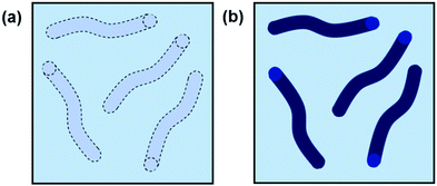Fig. 3 Cartoon example of worm-like micelles in solution with (a) poor contrast and (b) good contrast.

For both SAXS and SANS, the scattering is an average representation of a sample. This means that for samples containing multiple different structures, the scattering profile will be a combination of the individual scattering patterns of the components. This also applies for polydisperse distributions of the same structures (i.e., a range of sizes of sphere). Monodisperse structures may show distinct features in the scattering curve which would not be seen if the sample was polydisperse.³⁰ This can be demonstrated by the calculated form factor scattering patterns for 40 nm long cylinders with 2 nm radius with and without a Gaussian polydispersity in radius (Fig. 4). Small angle scattering techniques can therefore be used as a measure of polydispersity in a sample.

Fig. 4 Calculated form factor scattering patterns (using SasView v5.0.4) of 40 nm long cylinders with a 2 nm radius both with (red circles and line) and without (black diamonds and line) polydispersity. The cylinder model available in SASView was used, with a Gaussian polydispersity in radius of 0.2 for the red circles form factor.

The pros and cons of X-rays and neutrons

There are pros and cons with both SAXS and SANS: SAXS is a technique that can be undertaken in the laboratory as well as at synchrotron sources and requires very little sample preparation. Using a high flux synchrotron source, SAXS patterns can be collected in seconds, which allows for high throughput measurements³¹ and also probing of dynamics of systems on this timescale. However, as SAXS relies on scattering which is proportional to atomic number, light elements (from which gels are commonly composed) do not always scatter well and particularly in in-house instruments can require exposure times of hours to collect good data.

Care must also be taken when exposing gel samples to powerful synchrotron X-rays that sample damage does not occur due to over exposure to the beam. SANS requires the use of a dedicated synchrotron or neutron spallation source, and to perform the contrast matching outlined below, careful preparation of deuterated materials is needed, which can be costly and time consuming. Neutron beams are also relatively low flux in comparison to X-rays, meaning sample exposure times will be longer. Nevertheless, it is the ability to do contrast matching which makes SANS such a powerful technique in probing specific structural detail such as arrangement in multicomponent systems or to identify self-assembled packing not accessible by SAXS, and which will be further discussed below.

Experiment design – what can you measure, what can’t you measure, and what should you measure

A key question when planning SAXS or SANS experiments is, what is trying to be learnt? Small angle scattering is not always appropriate, and other techniques may be favourable. Small angle scattering provides information on structures on the order of approximately 1–100 nm. This can include size, shape, radius of gyration, packing, surface roughness and concentration. Different ways to process and analyse the scattering data are used to obtain different information. That is not to say that all this information will be gained from every experiment. The information that can be extracted depends greatly on the sample in question. Often the fibre-like structures underpinning gel networks are longer than the length that can be measured by SAS but information on the fibre radius and morphology (i.e., ribbon-like or cylindrical) can be determined.

The concentration of scattering objects in a sample is another important consideration because low concentrations may lead to weaker scattering. This might be improved through larger path length measurement cells and longer data collection times. With highly concentrated samples, structure factor scattering may occur, which may or may not be desirable. When performing SANS experiments, it is common for researchers to use H₂O and D₂O interchangeably, assuming that there is no influence on the self-assembly. However, this is not always the case and It is important to confirm that any solvent changes made for the purposes of the SAS experiments do not greatly alter the self-assembled structure.^32,33

For gels, sample loading into the measurement cell is an important consideration. Ideally, gelation would be triggered within the measurement cell, resulting in a homogenous and isotropic gel. Some gelation methods require trigger diffusion which can be hindered within the confines of the often small measurement cell. To avoid this challenge, gels can be broken and pipetted into the measurement cell, but this assumes that the primary structures are unaffected. As such, in situ gelation triggers (for example, thermal or chemical triggers) are favourable. Chemical triggers are homogeneously mixed prior to loading into the measurement cell, in which gelation then occurs slowly. For thermal triggers, the solution can be loaded into the cell prior to heating (assuming the cell can be heated!). Another consideration is that anisotropic ordering of the one dimensional structures within a gel can occur either by shear-alignment of one dimensional structures during loading or the confinement in small measurement cells.³⁴ The corresponding two dimensional scattering pattern will therefore show anisotropic scattering.

How small angle scattering methods can be employed

Data analysis – what the different plots can tell you

Here, we will discuss the different methods used to analyse small angle scattering data. An important consideration is that most analysis methods work on certain assumptions. For example, form factor model fitting assumes that the scattering object is dilute, isotropic, and non-interacting. For concentrated or more ordered systems, this may not be the case. When collecting scattering data on gels, we are interested in the shape and dimensions of the self-assembled objects which form the gel network (which are found by fitting the form factor, examination of the Guinier plot, and considering their polydispersity), the flexibility of the system (from the Kratky plot), particle–particle interactions (from consideration of the structure factor) and any evidence of ordering (shown by the presence of Bragg peaks).

The raw scattering pattern is a combination of scattering from the self-assembled structures, solvent, sample holder (e.g., capillary or cuvette) and air. Background subtractions must be performed to obtain the scattering arising solely from the self-assembled structures. A good background subtraction is important for good quality analysis of scattering data. In order to perform an accurate background subtraction, a scattering pattern of the empty cell, the cell containing the solvent and the cell containing the sample should be collected. The empty cell scattering should be subtracted from both solvent and sample before finally subtracting the solvent background from the sample. It is also crucial that the solvent be truly representative of the solvent used in the sample – for example, if the solvent is water, then a sample of the water used to prepare a sample should be used as the background, not simply any sample of distilled water.

Scattering data is typically first presented as a scattering intensity vs scattering vector plot (I vs. Q plot) on a log–log scale. A first question is, has the sample scattered effectively? Low scattering intensity with high error bars can indicate insufficient contrast or a lack of self-assembled structure present. Next, a preliminary analysis can be done by eye. The intensity and shape of the data as well as the slope in different regions all give information about the sample. Different shapes give characteristic slopes in the data at intermediate Q. The range over which the power law for a rod (as most of the systems we describe here are) is at Q between 1/L and 1/D where L is the length of the rod, and D is the diameter of the rod. Similarly for a disc, this region falls within the Q range between 1/D and 1/t where t is the disc thickness.

In Fig. 5, the theoretical scattering data for spherical, lamellar, and cylindrical structures have been plotted. Spherical structures give a slope of Q⁻⁴, disk-like and lamellar structures give a slope of Q⁻² and cylindrical structures give a slope of Q⁻¹. According to Porod's law, at high Q, a Q⁻⁴ decay is indicative of scattering from well-defined and sharp interfaces.^20,35 For all three structures, this is seen at >0.1 Å. The cylinder and the sphere form factors exhibit a plateau at low Q which is related to the absolute size of the object. Distinct oscillations can also be seen in the data at high Q which are related to the particle size and are also indicative of monodisperse structures.

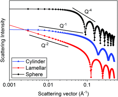Fig. 5 Calculated scattering patters (using SasView v5.0.4) for monodisperse spheres (radius = 50 Å), lamellae (thickness = 50 Å) and cylinders (radius = 20 Å and length = 400 Å).

A common approach to analysing small angle scattering data is model fitting.^21,36,37 This involves fitting the data to a model using fitting software. There are a range of software packages available, such as SasView and SasFit.^38,39 A wide range of models are available including shape independent models (such as a power law), form factor models (for example, a flexible cylinder) and structure factor models (such as interacting hard spheres). By assessing the slope at intermediate Q and/or with prior information about the shape of scattering objects (such as TEM images),^37,40 a broad class of models (such as cylinder models) can be chosen.

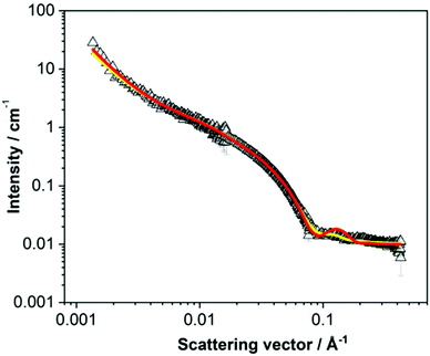
Fitting should be attempted to a range of different models within a class, starting with more simplistic models to avoid overfitting. Each model contains a range of parameters. If required, values for the material and solvent scattering length density are put into the fit and fixed for the fitting process. Models typically have a scale (volume fraction) parameter which scales the fit to the data. In quantitative measurements, the scale is related to the sample concentration. A first step in fitting involves initially fitting the scale and then the scale and the background parameter. Fitting to the correct background is crucial for a good fit. For neutron scattering experiments, careful calculation of the scattering length density of the system under study should be performed – this is achievable using the in-built tools within the fitting software. Only scale or scattering length density should be allowed to refine in the fit – customarily the scattering length density is known, and it is the scale that is fitted. Next, a procedure of fitting the individual model parameters (such as cylinder length and radius) to slowly improve the fit is performed. Finally, when the fit is close to the data, all parameters are fitted together. The goodness of fit at this point determines whether the chosen model is appropriate. Goodness of fit is determined through a combination of means including statistics (such as the reduced χ²), the fit residuals and by eye. If the chosen model fit is not near the data, does not capture key features (such as oscillations), or has a high reduced χ² a different model or polydispersity may be required. Different models within a class should be tried until a good fit is achieved. The model which achieves the best fit is taken to best depict the structures within the sample but it is crucial to assess if the obtained fitting parameters realistically depict the structures. For example, Fig. 6 shows SANS data that was ultimately best fit to a combined model of a cylinder and power law.⁴¹ The two fit lines show hollow cylinder model fits before (red) and after (yellow) fitting the thickness and radius of the hollow cylinder. Before fitting, a clear bump can be seen in the fit at high Q. After fitting, the hollow core radius fits to a value close to zero and the bump goes. It is important to note that the reduced χ² for this fit was sufficiently low, but the fit parameters depicted a sub-Angstrom hollow core radius! Hence, this gives a strong indication that the cylindrical structures do not have a hollow core and affirms the choice of just a cylinder model.

Fig. 6 An example where a model gives a sufficiently low reduced χ² value, but the fit depicts unrealistic structures. Here, both fit lines depict hollow cylinders before (radius = 16 Å, thickness = 21 Å and length = 349 Å, red line) and after (radius = 0.01 Å, thickness = 42 Å and length = 349 Å, yellow line) fitting the radius and thickness. In this instance the yellow fit has a reduced χ² of 1.55 and the red fit a reduced χ² of 4.73. Reproduced from ref. D. Giuri, L. J. Marshall, B. Dietrich, D. McDowall, L. Thomson, J. Y. Newton, C. Wilson, R. Schweins and D. J. Adams, Chem. Sci., 2021, 12, 9720–9725., with permission from the Royal Society of Chemistry.

In some cases, two different models may both give a sufficiently low reduced χ². Here studying the fit by eye may assist in the selection of the most appropriate model. Of course, in some cases, it is appropriate to simply record that either model effectively captures the data, and it is not possible to differentiate based on model fitting.

Care must be taken to avoid overfitting which is typically judged by having a reduced χ² of less than 1. Achieving a statistically good fit may not mean that it accurately depicts the sample. With more complex models containing many parameters, it is likely that a statistically good fit could be achieved to any set of data. Therefore, it is important to exercise caution and keep the models simplistic to start with to avoid overfitting. Combined models can also be used to fit the data where necessary. For example, a combined model depicting both a cylinder and sphere has been used to fit SAXS data of worm-like micelles.⁴² Different forms of cylinder model have been widely used to fit SAS data of low molecular weight gels and self-assembled fibres where the cylinder parameters correlate to the dimensions of the self-assembled fibres.^43–45 In low molecular weight gels, the length of the 1D structures that form frequently exceed the maximum length scale accessible by the SAS experiment. Therefore it is not possible to obtain a meaningful fit to the length parameter and additional techniques, for example, TEM, should be used to demonstrate the length of the gel fibres.

Sample polydispersity is commonly encountered in the real-world and can be accounted for in model fitting software, where different functions are often available. Apparent polydispersity can also be a product of limited experimental resolution.³⁰ Polydispersity should be used sparingly to avoid overfitting, however for soft matter systems, a Schulz-Zimm (referred to as the Schulz distribution in SASView) or the Gaussian polydispersity function are the most appropriate to apply.

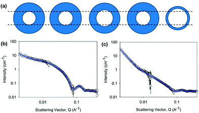
Model fitting should not be viewed as a solution to the analysis of all small angle scattering data. It has limitations and the context in which the analysis is done must be considered. Collected data may not be adequately fitted to a single model. For example, SAXS data for a specific functionalised dipeptide is best fit to a flexible cylinder model but SANS data for the same solution is best fit to a hollow cylinder.⁴⁶ The difference arises in the use of deuterated solvents providing better contrast in SANS and so the core is “seen” (Fig. 7).

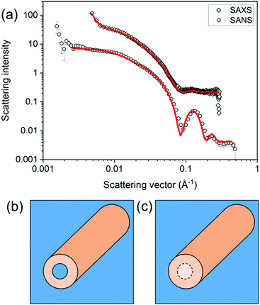Fig. 7 Differences in the model best capturing the data can arise from differences in the SLD. Here, (a) a flexible cylinder model (radius = 40.5 Å, length = 950 Å and Kuhn length = 63 Å) best captures the SAXS data for a sample prepared from a functionalised dipeptide, but the SANS data are best fit to a hollow cylinder model (radius = 37 Å, core radius = 19 Å and length = 401 Å).⁴⁶ This can be explained by contrast differences where the core does have contrast when using SANS (b) or does not have contrast by SAXS (c). Fig. (a) redrawn from E. R. Draper, H. Su, C. Brasnett, R. J. Poole, S. Rogers, H. Cui, A. Seddon and D. J. Adams, with permission from Wiley-VCH Verlag GmbH & Co. KGaA (Copyright © 2017) under the Creative Commons CC-BY (version 4.0) license.

Low Q – Guinier analysis. The Guinier analysis method is used to calculate radius of gyration (R_g) for scattering objects.⁴⁷ This involves analysing the data at small scattering vectors. The slope of a Guinier plot (ln I(Q) vs. Q²) at low Q is fitted to give the R_g. The Guinier relationship is given in eqn (3).

I(Q) = I(0)exp(Q²R_g²/−3) (3)

Here I(Q) is the intensity at a given scattering vector, I(0) is the scattering intensity at Q = 0, Q is the scattering vector and R_g is the radius of gyration. The Guinier analysis can be applied to a range of particle shapes but should only be applied to dilute, isotropic and monodisperse samples.⁴⁸ The Q_min and Q_max over which the data are fitted must be chosen appropriately to get good results. Deviation from linearity in the Guinier region may prevent a good fit, although this deviation can be informative because it indicates sample polydispersity or aggregation. For example, a “roll-over”/peak in the Guinier plot (Fig. 9) has been attributed to fibre aggregation in low molecular weight gels.^40,49 The Guinier analysis is often unsuitable for the very elongated 1D structures found in low molecular weight gels therefore modified Guinier plots have been used. The use of a modified Guinier plot, for example to measure the thickness of a sample with an anisotropic cross-section, and the equations which govern this fit can be found in work by Terech.^40,50 An excellent overview of the application of the Guinier Law to non-spherical objects is given by Beaucage.⁵¹

The cross-sectional radius of gyration of rod-like structures in β-sheet self-assembled hydrogels has been calculated and from this the cross sectional radius derived.⁵² Terech and co-workers have fitted small angle scattering data of low molecular weight gels to modified Guinier plots for both ribbon-like structures⁴⁰ and lamellar-like structures.⁵⁰ The Guinier analysis has limitations because the radius of gyration does not fully describe the size and the form of the structure under study. Rather it provides a characteristic geometrical parameter⁴⁷ and further analysis can be done to learn more about the sample.

Fractal analysis. As previously described, at intermediate Q the slope of the data can be related to the particle dimensionality. This can be described by a power law (eqn (4))

I(Q) ∼ Q^α (4)

where the power law decay takes non-integer values, a fractal analysis may be appropriate. A fractal is a structure which appears the same regardless of the length scale on which it is studied.⁵³ Having started as a mathematical concept, it has been applied in the real-world and is used in small angle scattering analysis. In practice, a fractal cannot be applied over every length scale but is relevant within a defined size range. Fractal analysis has been used for self-assembled gel systems.⁵⁴ When using fractal analysis in small angle scattering the slope, α, is used to extract fractal information. There are two types of fractal system relevant to small angle scattering, mass fractals and surface fractals. Mass fractals are typically aggregates of structures that persist throughout the system. Surface fractals are found only at the boundary of the fractal. Depending on the slope, the fractal can be assigned either a mass fractal or surface fractal.

When α is between 3 and 4, scattering is assigned to be from a surface fractal.^35,53 The surface fractal dimension, D_s, is then determined by eqn (5).

D_s = 6 − α (5)

Porod's law states that for scattering objects with sharp interfaces, the scattering decreases with Q⁻⁴ in the high Q region.^20,35 As such, for well-defined interfaces, D_s takes a value of 2. For increasingly less well defined (or rougher) interfaces, D_s is larger.

For mass fractals, α takes a value between 1 and 3 and the mass fractal dimension, D_m, is given by eqn (6).

D_m = α (6)

Mass fractal scattering occurs from structures of a self-similar nature (across the size range on which the fractal analysis is applied) and has been used to analyse scattering data for self-assembled gels. For example, a mass fractal analysis has been used to understand the compactness/density of fibril structures in the gel network at different concentrations.⁵⁴

Kratky analysis. The Kratky plot, whilst more commonly encountered in protein solution scattering where it is used to get a measure of the compactness of a protein, can also be used to analyse gel networks (Fig. 8). A Kratky plot can be used as evidence for branched structures as are commonly seen in gels. By plotting data on a Kratky plot, as Q²I(Q) against Q, features at high Q are highlighted and examination of the slope of the high Q region can confirm the conformation of the scattering objects. The shape of the Kratky plot provides an indication of the Gaussian chain nature of the material. At high Q, a Kratky plot of a Gaussian chain will become horizontally asymptotic, as I(Q) ∼ 1/Q². A stiff chain will continue to increase linearly at high Q, whereas a branched structure, such as a mass fractal will increase to a maximum then decrease as 1/Q at high Q. If the scattering is from three-dimensional objects, the high Q data will take the form I(Q) ≈ 1/Q⁴.⁵⁵ At low Q, in many cases a large peak in the Kratky plot can be observed which corresponds to spatial inhomogeneity within the gel.⁵⁶

Fig. 8 Kratky plot of a “slide-ring” gel which is based on a polyrotaxane consisting of poly(ethylene glycol) and α-cyclodextrin. M20, M60 and M80 denote the degree of methylation on the α-cyclodextrin, where the number represents the percent methylation, used in sample preparation. Reprinted from T. Karino, M. Shibayama, Y. Okumura and K. Ito, Phys. B, 2006, 385–386 I, 807–809. Copyright © 2006, with permission from Elsevier.

Contrast matching. An extremely powerful technique in SANS experiments is contrast matching, which uses the differences in SLD between different types of atoms, most commonly between hydrogen and deuterium. For example, H₂O and D₂O have very different SLDs of −0.561 × 10⁻⁶ Å⁻² and 6.393 × 10⁻⁶ Å⁻² respectively. Contrast matching has been applied to many systems, including surfactants and self-assembled gels.^57–59 SANS experiments are commonly performed in deuterated solvents for improved contrast. By selectively replacing the hydrogen atoms with deuterium atoms in all or part of the material under study, the contrast from those parts of the material is similar to that of the deuterated solvent. The contrast is therefore reduced and contributions from these parts of the material are effectively absent from the scattering pattern. Contrast matching can also be performed with partially deuterated compounds. This has been used to probe the self-assembly of a single LMWG⁶⁰ as well as to probe multicomponent gels to determine whether the components are self-sorted or co-assembled.⁵⁸ In a two-component self-assembled gel in a deuterated solvent, if one of the gelators is deuterated, the SANS pattern will arise solely from the non-deuterated gelator. If the two components are self-sorted, the scattering pattern should look identical to the un-deuterated component alone. Similarly, it is possible to contrast match out one of the components by mixing hydrogenated and deuterated solvents in different ratios to match the scattering length density to that of one of the components.⁶¹ We stress that these experiments are complex and typically require other techniques to reinforce any conclusions from the SANS data.

Structure factors. When working with gels, it is generally assumed that the concentration of scattering objects is sufficiently low to place the sample in the dilute regime, where interactions between scatterers can be neglected and no structure factor contribution is required to fit the data. However, in certain circumstances, this may not be true. In gel systems, the structure factor can often be adequately described by an Ornstein-Zernike (OZ) function at low Q, which takes into account the correlation length between the gel fibres in solution.⁶² It is also possible to use a Gaussian function to represent structure factor peaks from small-angle scattering data from gels.⁶³

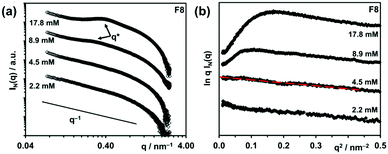
Peaks arising from the introduction of a structure factor can also be observed in I vs. Q plots and the position of the peak can be related to size through the Bragg relationship (d = 2π/Q). For example, from the position of the structure factor peaks in SAXS data (Fig. 9a), the hydrogel mesh size for a β-sheet forming peptide at two concentrations was estimated.⁴⁹ The mesh size decreased with increasing concentration, which is attributed to an increased fibre density. The data also showed a “roll-over” at low Q in a modified Guinier plot (Fig. 9b), which is attributed to interactions between fibres (aggregation).

Fig. 9 SAXS data of β-sheet forming peptide F8 studied by Wychowaniec et al. (a) I vs. Q plot with structure factor peaks indicated by q* (b) Guinier representation of the same data. Red dashed line shows the fit used to obtain the fibre cross-section radius of gyration. A roll-over is seen for the 8.9 and 17.8 mM data. Adapted with permission from J. K. Wychowaniec, A. M. Smith, C. Ligorio, O. O. Mykhaylyk, A. F. Miller and A. Saiani, Biomacromolecules, 2020, 21, 2285–2297. Copyright © 2020 American Chemical Society (ACS). Further permissions related to this material must be directed to the ACS.

Bragg peaks. In certain circumstances, even in a fully hydrated state, gels can be sufficiently well organised into repeating structures that peaks are seen within the scattering pattern in the mid to high Q region.^1,64–66 In-depth molecular packing can be investigated with wide angle X-ray scattering but this will not be discussed here.⁶⁴ For example, SANS data of a functionalised 2,3-didecyloxyanthracene organogels showed intense high Q Bragg peaks, indicating the formation of large, crystalline aggregates with extended molecular order.⁴⁰ The gelators that did not exhibit Bragg peaks were categorised as amorphous. Solutions of thiophene–diketopyrrolopyrrole conjugated to an octapeptide in solution showed the presence of self-assembled fibres with the width of approximately two extended molecules combined.⁶⁷ A Bragg peak in the SAXS data correlated to the extended length of 1 molecule and was indicative of a highly ordered and periodic arrangement. In other work, a Bragg peak was observed in SANS data for synthetic bile salt hydrogelators.⁵⁰ In these cases, it is necessary to exclude the Bragg peak from the form factor fitting, which depicted monodisperse rigid cylinders with diameters of 92 Å. The Bragg peak corresponded to around 16.5 Å which correlates with the molecular length of the component molecules. From this, it was deduced that the packing mode involves up to 25 molecules in a cross-sectional repeating unit.

Some case studies

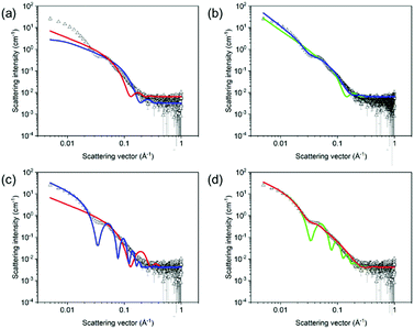
Here, we focus on specific case studies, chosen to bring together the concepts from above. We aim to show how small angle scattering methods can be used (and brought together with ancillary data) to understand low molecular weight gels. We stress that the choices are not meant to imply that these are the “best” gelators! First, we lead the reader through a specific example to show how to approach treating small angle scattering data.

A fitting case study. As an example of how to approach fitting data, we have chosen here one dataset from our lab. This dataset was difficult to fit and so we have chosen this as a case study. The data were collected from a mixture of the (L,L)-2NapFF and (D,D)-2NapFF. Each individual component forms a micellar solution that scatters as described above, forming hollow cylinders. The mixture however scatters differently from the SANS data from what would be expected from a superposition of the data for the single components (Fig. 10a). We fitted these data using SASView version 4.2.2.

Fig. 10 SANS data of the (L,L)-2NapFF/(D,D)-2NapFF mixture in D₂O (black hollow triangles) with corresponding attempted fits of (a) cylinder model with scale and background fitted (red line) and cylinder model with radius and length also fitted (blue line); (b) flexible cylinder model (green line) and flexible elliptical cylinder fit (blue line); (c) hollow cylinder model fitted (red line) and hollow cylinder model fitted after manually increasing radius and thickness (blue line); (d) hollow cylinder model with a Schulz polydispersity of radius with a value of 0.5 (red line) and a Schulz polydispersity of thickness with a value of 0.5 (green line).

The viscosity data showed that the solution was significantly more viscous than water. Additionally, cryo-TEM data showed that there were long anisotropic structures. Considering these data, it is appropriate to use cylinder-based models for these SANS data. Initially, a cylinder model was examined. Here, the SLD of the solvent was that for D₂O (6.393 × 10⁻⁶ Å⁻²) and a SLD for the mixture was 2.73 × 10⁻⁶ Å⁻², determined from the molecular formula and an assumed density of 1.53 g cm⁻³. The SLD parameters were input into the fitting software and kept constant throughout the fitting. If the SLD is not correct, this will affect the scale parameter, but not any of the size parameters. It is quite simple to check how significant this would be by manually changing the SLD and the scale values do not change dramatically over a sensible range of densities. Having set the SLD values, the scale and background were allowed to fit, keeping length and radius at the initial values (red fit, Fig. 10a). Having done this, the radius and lengths were also allowed to fit. From the final fit (blue data, Fig. 10a), it is clear that this fit does not capture the bump at around 5 × 10⁻² Å⁻¹. As such, this fit is not effective, and this can be seen from the high χ² value of 227.7.

Moving to a flexible cylinder model, all parameters were left to fit apart from the background, whilst keeping initially the extra parameter in this fit (the Kuhn length) as the initial value (100 Å). The χ² dropped immediately to around 95, which dropped further to 92 when the Kuhn length was also allowed to vary. This very high χ² value is due to the poor fit as can be seen from Fig. 10b (green data). Most importantly, the bump at around 5 × 10⁻² Å⁻¹ is not captured by the fit.

Similarly poor fits were obtained when using elliptical cylinder or flexible elliptical cylinder models. The lowest χ² was obtained with the flexible elliptical cylinder model, but it was still above 20 and the fit still does not capture the bump in the data (Fig. 10b, blue data).

Next, a hollow cylinder model was attempted, which depicts one dimensional tube-like structures. The model contains the following parameters: a core radius, the cylinder wall thickness, cylinder length, scale, background, SLD cylinder and SLD solvent parameters. The model assumes that the SLD inside the hollow cylinder is that of the bulk solvent. Again (after fixing the SLD values), the scale and background were allowed to vary whilst not changing the radius and thickness parameters. After this, the radius followed by the thickness were allowed to vary, giving outputted values of 13.6 and 10.7 Å respectively. The χ² is again high, and the fit is poor, again not capturing the bump at 5 × 10⁻² Å⁻¹ (Fig. 10c, red data). At this point, manual inputting of different values showed that a radius of 50 Å and a thickness of 20 Å gave a shape of curve that by eye captured the data better than any automated fit. The length was fitted to 5000 Å, a value significantly large to be outside the range of the measurement to represent long tubes. After this, allowing the scale, radius, and thickness to vary brought the fit close the data (Fig. 10c, blue data). However, the fit line implies that the data are significantly more polydisperse than the fit implies (see above). A Schulz polydispersity was therefore included in the fit. At this point, polydispersity in length, radius or thickness could be chosen. By manually inputting different values for the length, it is clear that beyond a certain value that there is little change in the fit and there is clearly no change in the resolution around the bump at 5 × 10⁻² Å⁻¹. As such, there is little point in including polydispersity for this parameter. Trying to include even relatively low values of polydispersity in both radius and thickness simultaneously results in extremely long times for the fitting to proceed and there is a tendency for errors to arise. As such, arbitrarily, a Schulz polydispersity in radius was chosen. A radius polydispersity parameter of 0.4 here (as a fixed value) and allowing radius and thickness to vary resulted in a good fit with a χ² of around 12. Increasing the Schulz polydispersity of radius parameter further to 0.5 slightly improves the χ² to around 11, with a radius 54.7 Å and a thickness of 20.4 Å (Fig. 10d, red data). Returning to the data without polydispersity and then examining only a Schulz polydispersity in thickness, the fit even with a parameter as high as 0.5 results in a much worse fit, with a χ² of 116 (Fig. 10d, green data).

Hence, on the basis of all of these fits, the hollow cylinder model with a high Schulz polydispersity in radius was deemed to be the best fit, as reported in the literature.⁶⁸ The data could be fitted to a core–shell model in which the scattering length density parameters are varied. If the hypothesis that hollow cylinders are formed is correct, the core SLD should fit to a value close to that of the solvent (in this case D₂O).

A modified dipeptide gelator. The next example we have chosen is again the modified dipeptide, (2S)-2-[(2S)-2-{2-[naphthalen-2-yloxy]acetamido}-3-phenylpropanamido]-3-phenylpropanoic acid, or 2NapFF for convenience. The chemical structure is shown in Fig. 11.

Fig. 11 Chemical structure of 2NapFF and variations where different parts of the chemical structure are deuterated; the deuterated sections are shown in red, and the abbreviation used in the text is shown under all structures.

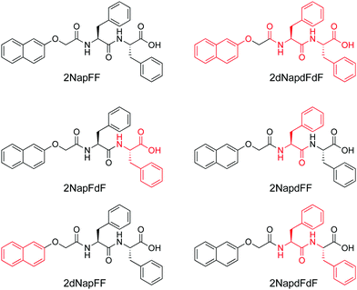
2NapFF can be dispersed in water at high pH by the addition of 1 molar equivalent of a base. Gels can also be formed by the addition of an acid.⁶⁰ It is expected that the 2NapFF will form self-assembled aggregates at high pH in water. At high pH, the carboxylic acid will be deprotonated, rendering some degree of hydrophilicity, but the remainder of the molecule will be hydrophobic. Hence, a surfactant-like nature is expected, and this is expected to be concentration dependent.

SANS and SAXS data were collected at high pH at a concentration of 10 mg mL⁻¹ (a standard concentration used for low molecular weight gelling samples). The SAXS measurements were carried out in both H₂O and D₂O, whilst the SANS measurements were carried out in D₂O to provide the necessary contrast. The first important point is that the SAXS data can be fitted to the same models whether the data are collected in H₂O or D₂O.⁶⁰ We highlight again that we showed that this is not always the case and so the common assumption that switching between H₂O and D₂O has a negligible effect is not always true for this kind of system.^32,33 The SAXS data for 2NapFF in D₂O can be fitted to a cylinder model or a flexible cylinder model; the fit to a cylinder model is similar in quality. The fit implies that the radius is 4.3 nm. The SANS data can be fitted to a hollow cylinder model combined with a power law (data shown in Fig. 7a). This power law allows the excess scattering at low Q to be taken into account. The wall thickness is found to be 2.1 nm and the core radius is found to be 1.65 nm. The core is not detected by SAXS due to the lack of contrast. Therefore, overall, SANS suggests that the radius is 3.75 nm. This is slightly smaller, but close to that found from the fit to SAXS data. The lengths derived from the fits are different but, in both cases, lie outside the Q range of the instrument.

We exploited contrast matching approaches to determine the packing of the 2NapFF in the aggregates at high pH.⁶⁰ First, we showed that the perdeuterated example (2dNap2F2F) scattered poorly in D₂O, but scatters well in H₂O (Fig. 12c). This was as expected, where contrast comes from the difference between the scattering length density of H and D as normal, except in this case it is the structure of interest that is deuterated. Fitting to the data in H₂O shows that the same hollow cylinder model combined with a power law can be used effectively and the radius, wall thickness and length are extremely close to the data found for 2NapFF in D₂O. This shows that the act of deuteration and the change from D₂O to H₂O does not affect the self-assembled structure formed. Similarly, the SAXS data for 2dNapFF and 2NapdFdF are very similar to the data for 2NapFF; this is expected if the self-assembled structures are unchanged in that SAXS should be insensitive to the deuteration. The SANS data however for the different variations are affected by the deuteration. Fitting of the data to a hollow cylinder model combined with a power law was possible in all cases, although the parameters obtained from the fit varied (Fig. 12a). For example, the fit to the data for 2dNapFF was almost identical to that of 2NapFF (Fig. 12b). The fit to the data for 2NapdFdF implies that the cylinder is very thin (Fig. 12a), with a wall thickness of 0.5 nm and a radius of 2.4 nm. Using these data, combined with cryo-TEM data and computational insight, we were therefore able to show that 2NapFF self-assembles into hollow tubes where the walls are formed by a bilayer.

Fig. 12 (a) Cartoon representation of hollow cylinder cross-sections obtained from the fitting of SANS data for (from left to right) 2NapFF, 2dNapFF, 2NaphFdF, 2NapdFhF and 2NapdFdF. SANS data for (b) 2dNapFF in D2O (second from left in cartoon) and (c) 2NapdFdF in D2O (far right in cartoon). Reproduced from E. R. Draper, B. Dietrich, K. McAulay, C. Brasnett, H. Abdizadeh, I. Patmanidis, S. J. Marrink, H. Su, H. Cui, R. Schweins, A. Seddon, D. J. Adams, Matter, 2020, 2, 3, 764–778, with permission from Elsevier (Copyright © 2020) under the Creative Commons CC-BY (version 4.0) license.

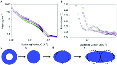
Gels can be formed from 2NapFF by lowering the pH. By adding glucono-δ-lactone (GdL) to a solution of 2NapFF, the slow hydrolysis of GdL to gluconic acid allowed us to follow the gelation with time.⁶⁰ We were able to determine that the first thing that happens is that the core of the hollow cylinder collapses. This correlates with the observation that the solutions prepared from 2NapFF have two apparent pK_a values, which we ascribe to the carboxylates pointing into the core of the tubes and to those on the external surface of the tubes. Following this, the data can be fitted to a cylinder model, which gradually needs increased polydispersity to be well fitted. At later times, the best model is an elliptical cylinder. We therefore can use these data to determine that the core collapses, cylinders are formed which then laterally associate to form structures which are elliptical in cross-section (Fig. 13). This hypothesis explains why similar data collected on the partially deuterated analogues does not give well-defined structures; if collapse leads to relatively disordered packing, there will not be well-defined sections within the aggregates that are deuterated.

Fig. 13 (A) SANS for 2NapFF before addition of GdL (black), 15 min after addition (green), and 180 min after addition (purple). (B) shows an expansion of the data in (A) to show the disappearance of the peak at high Q. From these data, the fits show that as the pH is decreased, the hollow cylinders formed by 2NapFF initially lose the core before becoming elliptical. (C)–(F) show in cartoon format (drawn to scale) how the structures evolve from hollow tubes to elliptical cylinders as the gelation proceeds. Reproduced from E. R. Draper, B. Dietrich, K. McAulay, C. Brasnett, H. Abdizadeh, I. Patmanidis, S. J. Marrink, H. Su, H. Cui, R. Schweins, A. Seddon, D. J. Adams, Matter, 2020, 2, 3, 764–778, with permission from Elsevier (Copyright © 2020) under the Creative Commons CC-BY (version 4.0) license.

A β-Hairpin gelator. Pochan's group have collected significant data on a family of peptides that form gels via folding into β-hairpins.⁶⁹ For example, three different 20 amino acid peptide sequences that fold into β-hairpins have been studied, denoted SSP1, SSP2 and SSP3; the exact sequences can be found in the original reference but the critical point is that all form gels by self-assembly into fibrillar structures. Strand asymmetry was introduced to the β-hairpin structures resulting in free peptides at the end of the β-hairpin. The free peptide chains can overlap to form dimers and, given the correct trigger, the dimers self-assemble into fibril nanostructures forming a fibril network and self-supporting gel. The relationship between the network structure and the local fibril structure of self-assembled peptide gels was probed using SANS measurements, cryo-TEM and rheological measurements.

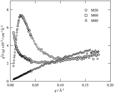
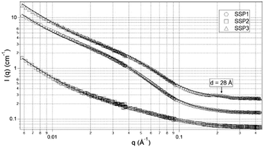
TEM images of gels from the three different peptides showed three distinctly different structures. SSP1 formed fibrils with regular twists, SSP2 forms untwisted fibrils and SSP3 laminated fibrils. SANS measurements of the three peptide gels were collected and showed three distinct scattering patterns (Fig. 14).

Fig. 14 SANS data for the β-hairpin peptides studied by Pochan's group. The open shapes show the data and the solid lines show the fits to the data as discussed in the text. Reprinted with permission from R. A. Hule, R. P. Nagarkar, B. Hammouda, J. P. Schneider and D. J. Pochan, Macromolecules, 2009, 42, 7137–7145. Copyright © 2009 American Chemical Society.

SSP3 showed a small peak at high Q, corresponding to a length of 28 Å. Combined with the TEM images, this peak was assigned to the width of a single filament within a laminated fibril. To fit the scattering data adequately a single expression could not be used. Instead, the scattering profiles of the peptide hydrogels were captured by a nonlinear least squares fit with the following expression (eqn (7)):

In this equation, B is the background scattering, A and C correspond to multiplicative factors for the two terms, L is the correlation length and n and m are scaling exponents. Within this equation, different terms cover the scattering at different Q regimes. The low Q regime is covered by A/Qⁿ, and covers scattering from the gel network, whereas the high Q regime is covered by the (C/1 + (QL)^m) term. They note that similar expressions have been used to fit data for polymer and polyelectrolyte systems.

The exponent n reflects low Q scattering occurring on the 100 s nm size range which is from the network. Here, all three peptides have a value of n = 1.7, which is assigned as scattering from fully swollen Gaussian chains in a good solvent. For SSP1 and 2, this is an appropriate analysis and suggests that the change to the peptide sequence does not influence the network structure. For SSP3 this is not appropriate due to the laminated structure. SSP1 and 3 have higher scattering intensities in the mid to high Q region which is attributed to both twisted and laminated fibrils being more compact, having a greater number of peptide molecules per unit length. This is reflected in the high Q exponent increasing from SSP2 (untwisted) to SSP1 (twisted). SSP3 possesses a high Q exponent of 3.62, which is assigned to power law scattering from well-defined interfaces. The correlation length is another parameter obtained from the model used. Moving from SSP2 (untwisted) to SSP3 (laminated), a decrease in correlation length from 20 to 16 was seen, which indicated a greater compactness within the nanostructure of SSP3.

A concentration study from 1 to 4 wt% was performed for SSP2 and SSP3. For SSP2, an increase in high Q exponent was seen with increasing concentration, indicating a greater degree of network compactness. This was reflected in cryo-TEM measurements of those gels. Conversely, SSP3 showed a decrease in the high Q exponent with increasing concentration. Again, the cryo-TEM measurements reflected this. This was attributed to the faster self-assembly kinetics associated with the higher concentration, leading to imperfections in the laminates.

This work serves to exemplify that subtle changes to the chemical structure within a class of similar molecules results in significant differences in the self-assembled structure. This in turn influences the network structure and bulk rheological properties.

A case study using Bragg peaks. While Bragg peaks are not always present in SAXS and SANS patterns of gels, their presence can greatly aid the understanding of the packing of molecules and gel fibres. A series of elegant experiments were carried out by Terech and co-workers using SANS to compare the structural characteristics of a series of orthodialkoxyarene organogelators.⁴⁰ Whilst not hydrogels (as the solvent here is ethanol), they serve as an excellent example of the richness of information that can be extracted from a scattering pattern to describe the structure of a self-assembled small molecule gel. By varying the aromatic moiety and chain length of a gelator molecule, the authors were able to create six new structurally related gelators and describe how these modifications affect their hierarchical assembly. In particular, the presence of Bragg peaks in the SANS data sheds light on how single gel fibres can pack to form larger bundles, and that in some cases, these bundles show crystalline ordering.

It can be seen from the SANS data (Fig. 15) that samples of organogel 5 (structure shown in Fig. 15a) do not display any ordering that would lead to the presence of Bragg peaks, and that the data can be modelled using a cylinder form factor with an anisotropic cross-section. However, modification of the cyclic skeleton to 3 (Fig. 15a) drastically changes the scattering which showed the presence of a strong Bragg peak (Fig. 15c), indicating molecular order even in the gel state. The peak at Q = 0.152 Å⁻¹ corresponds to a real space value of 41.3 Å, suggesting that the molecules of organogelator are overlapping and it is this that can explain how individual gel fibres can form in bundles. Thus, the presence of Bragg peaks can be used to explain the hierarchical assembly of these materials.

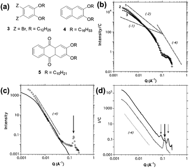Fig. 15 (a) Chemical structures of some of the organogelators studied by Terech et al.⁴⁰ (b) SANS data for organogelator 5 at 0.034 wt% (line 1, crosses), 0.043 wt% (line 2, solid line) and 0.1 wt% (line 3, circles). Dotted lines are guides for Q⁻¹, Q⁻² and Q⁻⁴ intensity decays. (c) SANS data for organogelator 3 at 1.09 wt% (open circles) with a Q⁻⁴ intensity decay (dotted line) and a radially polydisperse bundle of fibres form factor (solid line) The arrow guides the eye to the Bragg peak at Q = 0.152 Å⁻¹. (d) SANS data for organogelator 4 at 0.396 wt% (solid line) and 5.86 wt% (dotted line) with a Q⁻⁴ intensity decay (dashed line). Arrows guide the eye to Bragg peaks at 0.0857, 0.126 and 0.171 Å⁻¹. Fig. (b), (c) and (d) reprinted from P. Terech, G. Clavier, H. Bouas-Laurent, J. P. Desvergne, B. Demé and J. L. Pozzo, J. Colloid Interface Sci., 2006, 302, 633–642., Copyright © 2006, with permission from Elsevier.

Similarly, organogelator 4 (Fig. 15a) at low concentration shows the presence of three strong Bragg peaks (Fig. 15d), which correspond to molecular ordering on a square lattice. However, on increasing concentration, the three peaks are replaced by a single peak implying that the merging of fibres into bundles is chemically specific and growth of periodic structures happens along defined directions.

Conclusions

In this review, we hope that we have shown the power of small angle scattering for characterising and understanding low molecular weight gels. We have found that these techniques can add significantly to our understanding of such systems, with key advantages over other techniques such as the ability to carry out the analysis in the solvated state and providing information as to the bulk of the samples. These techniques are in our opinion significantly more useful than most microscopy techniques where drying is needed for example. Of course, the key drawback is the hurdle overcome in terms of accessing equipment time and understanding the methodologies available for analysing data. We hope that we have been able to at least reduce the barrier to using such techniques and inspire more people to use them for their systems.

Conflicts of interest

There are no conflicts to declare.

Acknowledgements

We thank the Leverhulme Trust for funding (RPG-2018-013). We would like to thank the many collaborators who have been critical in developing the understanding that we have for using small angle scattering to probe self-assembled gels. Most particularly, we would like to thank Dr Emily Draper (University of Glasgow), Professor Peter Griffiths (University of Greenwich), Dr Ralf Schweins (ILL) and Dr Steve King (ISIS) for their extensive help and insights over the last few years.

Notes and references

1. P. Terech and R. G. Weiss, Chem. Rev., 1997, 97, 3133–3159.
2. L. A. Estroff and A. D. Hamilton, Chem. Rev., 2004, 104, 1201–1217.
3. R. G. Weiss, Gels, 2018, 4(2), 25.
4. D. K. Smith, in Molecular Gels: Structure and Dynamics, ed. R. G. Weiss, Royal Society of Chemistry, Cambridge, 2018, pp. 300–371.
5. A. R. Hirst, B. Escuder, J. F. Miravet and D. K. Smith, Angew. Chem., Int. Ed., 2008, 47, 8002–8018.
6. K. J. Skilling, F. Citossi, T. D. Bradshaw, M. Ashford, B. Kellam and M. Marlow, Soft Matter, 2014, 10, 237–256.
7. S. Panja, A. Panja and K. Ghosh, Mater. Chem. Front., 2021, 5, 584–602.
8. K. Sugiyasu, S. Kawano, N. Fujita and S. Shinkai, Chem. Mater., 2008, 20, 2863–2865.
9. S. S. Babu, V. K. Praveen and A. Ajayaghosh, Chem. Rev., 2014, 114, 1973–2129.
10. E. R. Draper and D. J. Adams, Chem. Soc. Rev., 2018, 47, 3395–3405.
11. V. J. Nebot and D. K. Smith, in Functional Molecular Gels, ed. H.-J. Butt, I. W. Hamley, H. A. Stone and C. Wu, The Royal Society of Chemistry, Cambridge, 1st edn, 2014, pp. 30–66.
12. G. Yu, X. Yan, C. Han and F. Huang, Chem. Soc. Rev., 2013, 42, 6697–6722.
13. A. Rizvi, J. T. Mulvey, B. P. Carpenter, R. Talosig and J. P. Patterson, Chem. Rev., 2021, 121(22), 14232–14280.
14. M. Galluzzi, G. Tang, C. S. Biswas, J. Zhao, S. Chen and F. J. Stadler, Nat. Commun., 2018, 9, 3584.
15. S. Pujals, N. Feiner-Gracia, P. Delcanale, I. Voets and L. Albertazzi, Nat. Rev. Chem., 2019, 3, 68–84.
16. S. Onogi, H. Shigemitsu, T. Yoshii, T. Tanida, M. Ikeda, R. Kubota and I. Hamachi, Nat. Chem., 2016, 8, 743–752.
17. G. A. Roth, S. Tahiliani, N. M. Neu-Baker and S. A. Brenner, Wiley Interdiscip. Rev.: Nanomed. Nanobiotechnol., 2015, 7, 565–579.
18. L. L. E. Mears, E. R. Draper, A. M. Castilla, H. Su, Zhuola, B. Dietrich, M. C. Nolan, G. N. Smith, J. Doutch, S. Rogers, R. Akhtar, H. Cui and D. J. Adams, Biomacromolecules, 2017, 18, 3531–3540.
19. T. Xia, W. Liu and L. Yang, J. Biomed. Mater. Res., Part A, 2017, 105, 1799–1812.
20. J. B. Guilbaud and A. Saiani, Chem. Soc. Rev., 2011, 40, 1200–1210.
21. M. J. Hollamby, Phys. Chem. Chem. Phys., 2013, 15, 10566–10579.
22. T. Narayanan and O. Konovalov, Materials, 2020, 13(3), 752.
23. C. J. Gommes, S. Jaksch and H. Frielinghaus, J. Appl. Crystallogr., 2021, 54, 1–12.
24. I. W. Hamley, Small-Angle Scattering: Theory, Instrumentation, Data, and Applications, John Wiley & Sons, Chichester, 1st edn, 2021.
25. S. R. Bhatia, Curr. Opin. Colloid Interface Sci., 2005, 9, 404–411.
26. P. N. Pusey, in Neutrons, X-rays and Light Scattering Methods Applied to Soft Condensed Matter, ed. T. Zemb and P. Lindner, North Holland, 1st edn, 1988.
27. O. Glatter and O. Kratky, Small Angle X-ray Scattering, Academic Press, London, 1982.
28. L. A. Feigin and D. I. Svergun, Structure Analysis by Small-Angle X-ray and Neutron Scattering, Plenum Press, New York, 1st edn, 1987.
29. J. Jiang, F. P. E. Dunne and T. Ben Britton, JOM, 2017, 69, 863–871.
30. F. X. Simon, T. T. T. Nguyen, N. Díaz, M. Schmutz, B. Demé, J. Jestin, J. Combet and P. J. Mésini, Soft Matter, 2013, 9, 8483–8493.
31. N. P. Cowieson, C. J. C. Edwards-Gayle, K. Inoue, N. S. Khunti, J. Doutch, E. Williams, S. Daniels, G. Preece, N. A. Krumpa, J. P. Sutter, A. D. Tully, N. J. Terrill and R. P. Rambo, J. Synchrotron Radiat., 2020, 27, 1438–1446.
32. K. McAulay, H. Wang, A. M. Fuentes-Caparrós, L. Thomson, N. Khunti, N. Cowieson, H. Cui, A. Seddon and D. J. Adams, Langmuir, 2020, 36, 8626–8631.
33. T. R. Canrinus, F. J. R. Cerpentier, B. L. Feringa and W. R. Browne, Chem. Commun., 2017, 53, 1719–1722.
34. P. Terech, J. J. Allegraud and C. M. Garner, Langmuir, 1998, 14, 3991–3998.
35. T. Suzuki, A. Chiba and T. Yano, Carbohydr. Polym., 1997, 34, 357–363.
36. C. Yan, A. Altunbas, T. Yucel, R. P. Nagarkar, J. P. Schneider and D. J. Pochan, Soft Matter, 2010, 6, 5143–5156.
37. A. D. Martin, J. P. Wojciechowski, A. B. Robinson, C. Heu, C. J. Garvey, J. Ratcliffe, L. J. Waddington, J. Gardiner and P. Thordarson, Sci. Rep., 2017, 7, 1–6.
38. SasView, https://www.sasview.org/, (accessed 21 September 2021).
39. SasFit, https://sasfit.org/, (accessed 21 September 2021).
40. P. Terech, G. Clavier, H. Bouas-Laurent, J. P. Desvergne, B. Demé and J. L. Pozzo, J. Colloid Interface Sci., 2006, 302, 633–642.
41. D. Giuri, L. J. Marshall, B. Dietrich, D. McDowall, L. Thomson, J. Y. Newton, C. Wilson, R. Schweins and D. J. Adams, Chem. Sci., 2021, 12, 9720–9725.
42. O. Nahi, O. J. Cayre, Y. Y. Kim, A. J. Smith, N. J. Warren and F. C. Meldrum, Chem. Commun., 2020, 56, 7463–7466.
43. J. Li, Y. Zhao, P. Zhou, X. Hu, D. Wang, S. M. King, S. E. Rogers, J. Wang, J. R. Lu and H. Xu, Small, 2020, 16, 1–11.
44. H. Kumari, S. E. Armitage, S. R. Kline, K. K. Damodaran, S. R. Kennedy, J. L. Atwood and J. W. Steed, Soft Matter, 2015, 11, 8471–8478.
45. I. W. Hamley, A. Dehsorkhi, V. Castelletto, S. Furzeland, D. Atkins, J. Seitsonen and J. Ruokolainen, Soft Matter, 2013, 9, 9290–9293.
46. E. R. Draper, H. Su, C. Brasnett, R. J. Poole, S. Rogers, H. Cui, A. Seddon and D. J. Adams, Angew. Chem., Int. Ed., 2017, 56, 10467–10470.
47. A. Guinier and G. Fournet, Small-Angle Scattering of X-rays, John Wiley & Sons, New York, 1955.
48. P. Terech, W. G. Smith and R. G. Weiss, J. Chem. Soc., Faraday Trans., 1996, 92, 3157–3162.
49. J. K. Wychowaniec, A. M. Smith, C. Ligorio, O. O. Mykhaylyk, A. F. Miller and A. Saiani, Biomacromolecules, 2020, 21, 2285–2297.
50. P. Terech, S. Dourdain, S. Bhat and U. Maitra, J. Phys. Chem. B, 2009, 113, 8252–8267.
51. G. Beaucage, J. Appl. Crystallogr., 1995, 28, 717–728.
52. R. V. Rughani, D. A. Salick, M. S. Lamm, T. Yucel, D. J. Pochan and J. P. Schneider, Biomacromolecules, 2009, 10, 1295–1304.
53. P. W. Schmidt, J. Appl. Crystallogr., 1991, 24, 414–435.
54. R. A. Hule, R. P. Nagarkar, A. Altunbas, H. R. Ramay, M. C. Branco, J. P. Schneider and D. J. Pochan, Faraday Discuss., 2008, 139, 251–264.
55. E. M. Saffer, M. A. Lackey, D. M. Griffin, S. Kishore, G. N. Tew and S. R. Bhatia, Soft Matter, 2014, 10, 1905–1916.
56. T. Karino, M. Shibayama, Y. Okumura and K. Ito, Phys. B, 2006, 385–386 I, 807–809.
57. D. Bendedouch, S. H. Chen and W. C. Koehler, J. Phys. Chem., 1983, 87, 153–159.
58. K. L. Morris, L. Chen, J. Raeburn, O. R. Sellick, P. Cotanda, A. Paul, P. C. Griffiths, S. M. King, R. K. O’Reilly, L. C. Serpell and D. J. Adams, Nat. Commun., 2013, 4, 1–6.
59. Y. B. Melnichenko and G. D. Wignall, J. Appl. Phys., 2007, 102, 021101.
60. E. R. Draper, B. Dietrich, K. McAulay, C. Brasnett, H. Abdizadeh, I. Patmanidis, S. J. Marrink, H. Su, H. Cui, R. Schweins, A. Seddon and D. J. Adams, Matter, 2020, 2, 764–778.
61. E. R. Cross, S. Sproules, R. Schweins, E. R. Draper and D. J. Adams, J. Am. Chem. Soc., 2018, 140, 8667–8670.
62. E. Geissler, F. Horkay, A.-M. Hecht, C. Rochas, P. Lindner, C. Bourgaux and G. Couarraze, Polymer, 1997, 38, 15–20.
63. V. Castelletto, R. Itri, L. Q. Amaral and G. P. Spada, Macromolecules, 1995, 28, 8395–8400.
64. J. R. Wester, J. A. Lewis, R. Freeman, H. Sai, L. C. Palmer, S. E. Henrich and S. I. Stupp, J. Am. Chem. Soc., 2020, 142, 12216–12225.
65. B. Mondal, D. Bairagi, N. Nandi, B. Hansda, K. S. Das, C. J. C. Edwards-Gayle, V. Castelletto, I. W. Hamley and A. Banerjee, Langmuir, 2020, 36, 12942–12953.
66. K. Basu, N. Nandi, B. Mondal, A. Dehsorkhi, I. W. Hamley and A. Banerjee, Interface Focus, 2017, 7, 20160128.
67. A. Rani, I. Kavianinia, P. Hume, L. M. De Leon-Rodriguez, S. Kihara, D. E. Williams, D. J. McGillivray, N. O. V. Plank, J. Gerrard, J. M. Hodgkiss and M. A. Brimble, Soft Matter, 2020, 16, 6563–6571.
68. K. McAulay, B. Dietrich, H. Su, M. T. Scott, S. Rogers, Y. K. Al-Hilaly, H. Cui, L. C. Serpell, A. M. Seddon, E. R. Draper and D. J. Adams, Chem. Sci., 2019, 10, 7801–7806.
69. R. A. Hule, R. P. Nagarkar, B. Hammouda, J. P. Schneider and D. J. Pochan, Macromolecules, 2009, 42, 7137–7145.

---