
Machine learning based interpretation of microkinetic data: a Fischer–Tropsch synthesis case study†
Anoop
Chakkingal
ab,
Pieter
Janssens
a,
Jeroen
Poissonnier
 a,
Alan J.
Barrios
ab,
Mirella
Virginie
b,
Andrei Y.
Khodakov
b and
Joris W.
Thybaut
*a
a,
Alan J.
Barrios
ab,
Mirella
Virginie
b,
Andrei Y.
Khodakov
b and
Joris W.
Thybaut
*a
aLaboratory for Chemical Technology (LCT), Department of Materials, Textiles and Chemical Engineering, Ghent University, Technologiepark 125, 9052 Ghent, Belgium. E-mail: joris.thybaut@ugent.be
bCNRS, Centrale Lille, Univ. Lille, ENSCL, Univ. Artois, UMR 8181 – UCCS – Unité de Catalyse et Chimie du Solide, F-59000 Lille, France
First published on 12th October 2021
Abstract
Machine-learning (ML) methods, such as artificial neural networks (ANNs), bring the data-driven design of chemical reactions within reach. Simultaneously with the verification of the absence of any bias in the machine learning model as compared to the microkinetic data, interpretation techniques such as permutation importance, SHAP values and partial dependence plots allow for a more systematic (model agnostic) analysis of these data. In the present work, this methodology is demonstrated for Fischer–Tropsch synthesis (FTS) on a cobalt catalyst, with methane yield as the single dominant output, as a case study. For the purpose of this case study, the dataset required for training the ANN model is synthetically generated using a single-event microkinetic (SEMK) model. With a number of 3 hidden layers with 20 nodes, the ANN model is able to adequately reproduce the SEMK results. The relative ranking of the process variables, as learnt by the ANN model, is identified using interpretation techniques, with the methane yield being most dependent on the temperature, followed by the space-time and syngas molar inlet ratio, in the investigated range of operating conditions. This is in line with the physicochemical understanding from SEMK. A systematic approach for analysing microkinetic data, generally analysed on a case-specific basis, is thus developed by combining more widely used interpretation techniques in data science with the ANN.
1 Introduction
With the increase in computational capacity and the ability to handle large volumes of data, high-throughput experimental trials, etc., there has been an increased interest in applying machine learning (ML) models to chemical engineering problems. ML methods are rapidly gaining popularity for modelling complex nonlinear process phenomena in the field of chemical engineering.1–4 ML is a sub-field of artificial intelligence, where information from the data is learnt using algorithms. Usage of different ML methods such as support vector machine (SVM), random forest and neural networks, etc. for classification and regression is being extensively investigated in different areas of chemical engineering such as electro-synthesis,5 biomass gasification,6 catalysis,7,8 molecular drug discovery,9,10etc. The data required for developing ML-based models are obtained from experiments4,11 or synthetically generated using computational models.12 These studies point at the increasing interest in ML-based models in different sub-fields in chemical engineering.Among the different techniques in machine learning mentioned above, artificial neural network (ANN) is one of the powerful predictive tools, which works on the principle based on the universal approximation theorem.13 ANN is used for both regression and classification. ANN relies on the collective working of the building units, i.e. the neurons.14 The functioning of these neurons is inspired by that of biological ones. Here, relationships or patterns are established from the dataset between the input and the output in the training stage, and the ANN model uses this information in the prediction stage. A neural network is considered a “black box” model, as it is difficult to interpret it in a fundamental manner when compared to models such as linear regression (Fig. 1).
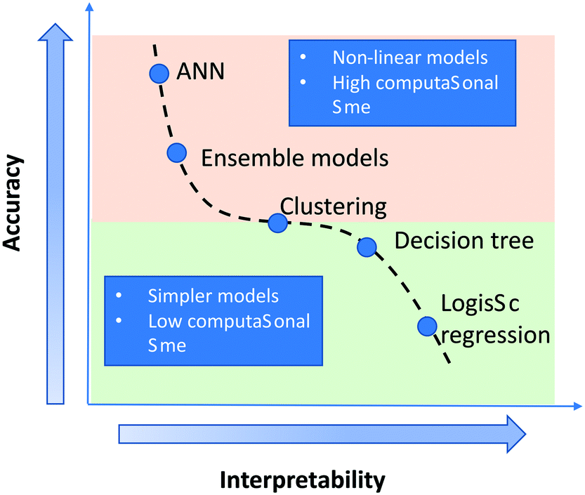 | ||
| Fig. 1 Graphical representation of variation in interpretability of a model with change in accuracy as reported in the literature.15 The interpretability of a model decreases with increase in accuracy and complexity of a model. | ||
A machine learning algorithm such as ANN predicts the outcome based on the information learnt from the training set. The applicability and validity of such a model for a process are currently based on accuracy measurements such as the mean square error, mean absolute error, etc. However, relying on these metrics alone can make them biased towards certain input features. Any bias in the dataset will be reflected in the model obtained from the algorithm. Thus, trusting the model also demands understanding why a certain decision is made by the model.
The identification of input features which exhibit the most pronounced contribution towards the target output prediction in the learning process of ANN is not straightforward. There is always a trade-off between prediction accuracy and interpretability of a model (see Fig. 1). For a “simple” model such as linear regression, the weights or coefficients associated with the independent features provide a direct quantitative measure for their importance in the model. As the model complexity increases from linear/logistic regression to neural networks, the prediction accuracy increases, but the interpretability decreases.15 To address this issue, with the recent advances in interpretation techniques,16 the interpretability of complex models such as ANN is being extensively investigated.
The most prominent interpretation techniques reported in the literature are permutation importance,17 SHAP values18–20 and partial dependence plots.21 The validity and explanation quality of these techniques depend on the situations in which they are used. Insights gained from different interpretation techniques allow revealing the relative impact of each input feature on the output. The combined effects and correlation of different input features may also be identified. The contribution of a particular feature in a multidimensional dataset can then be evaluated based on process expertise.22 At present, these interpretation techniques, which are model agnostic in nature, are mostly used in medicine,23–26 finance,27,28etc. However, the application of these techniques in the field of chemical modelling is currently under-explored.22 These techniques along with ML models can help in unravelling the hidden trends in kinetic data obtained from different chemical reactions and for their systematic analysis.
Fischer–Tropsch synthesis (FTS) is one such interesting chemical reaction where these techniques can be useful. FTS is widely investigated from synthesis gas that can be obtained from a wide variety of origins to synthesize hydrocarbons.29,30 The composition of non-petroleum-based hydrocarbons obtained via FTS depends upon a number of process features, such as the feedstock (syngas ratios obtained after gasification) nature, the catalyst used, and the process operating conditions. The FTS reaction has been widely investigated experimentally29,30via density functional theory31 and by different kinetic models.32,33 A single-event microkinetic model is one such versatile, comprehensive kinetic model developed to deal with complex mixtures34 in reactions such as hydrocracking,35 catalytic cracking,36 Fischer–Tropsch synthesis,37,38etc. The analysis of the kinetic data obtained with such models is usually carried out on a case-specific basis, demanding expertise in working with these models. In the recent decade, literature has also been reported on the use of ANN-based models for modelling the FTS.39–41 However, these studies are limited to the building of the neural network to predict the output components with limited focus on how each input feature plays a role in the prediction process.
In this work, a case study on the interpretation of a “black-box” ANN regression model developed from the microkinetic data corresponding to Fischer–Tropsch synthesis (FTS) is assessed with the help of different interpretation techniques mentioned above. This opens up the possibility of more systematic analysis and interpretation of kinetic data with the help of methods currently used widely in data science. The interpretability of ML models such as ANN can also build confidence in them to accurately predict results and draw chemical trends/insights. We could thus use them as an alternative to (micro)kinetic modeling and even to analyse the behavior of existing (micro)kinetic models using ‘non-classical’ contribution analysis techniques.
2 Procedures
2.1 Theoretical background
An ANN is an efficient data-driven model which can learn the hidden patterns in a dataset and transform input data into output.14As shown in Fig. 2, an ANN is composed of components called neurons (colored circles). A set of neurons is subsequently stacked to form layers, which are classified as:
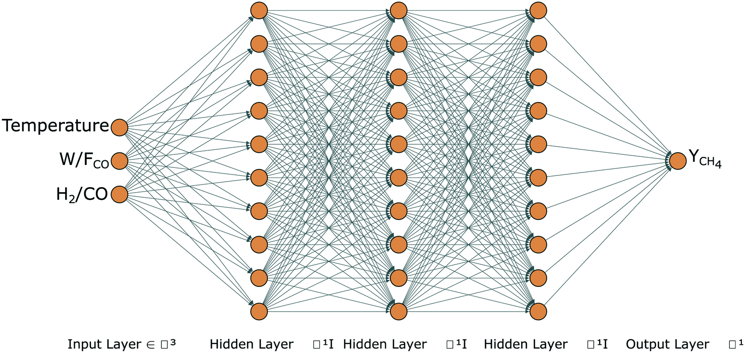 | ||
| Fig. 2 Schematic representation of an ANN consisting of 3 input features in the input layer, 3 hidden layers with 10 neurons in each layer and 1 output feature in the output layer. The input features in the representation are temperature, space-time (W/FCO) and syngas molar inlet ratio (H2/CO) and the output is methane yield (YCH4). | ||
• Input layer: contains the input features, i.e., for the FTS process: temperature, space-time and syngas molar inlet ratio.
• Hidden layer(s): the layer(s) of neurons between the input and the output layers.
• Output layer: the layer of neurons that corresponds to the (predicted) output of the model, i.e. methane yield for the current FTS process.
The output is generated by assigning weights to the neurons and applying activation functions to the input, output and hidden layers. The connections between the neurons have a weight that does a linear transformation on the input value, while the activation function does a non-linear transformation. Although there are different types of activation functions, the most conventional ones are the sigmoid and the rectified linear unit (ReLU) for the input (and output) and the hidden layers, respectively.14 The sigmoid activation function ensures that the network captures the non-linearity of the input–output relation, while the ReLU activation function in the hidden layers effectively avoids the vanishing gradient problem.42
The output values at each iteration, also denoted as epoch in the field, are obtained after the input information is fed via a feed-forward propagation. A back-propagation algorithm is used to train the neural network by recalculating the revised weights based on the error obtained from the output value.
2.2 Artificial neural network construction and analysis
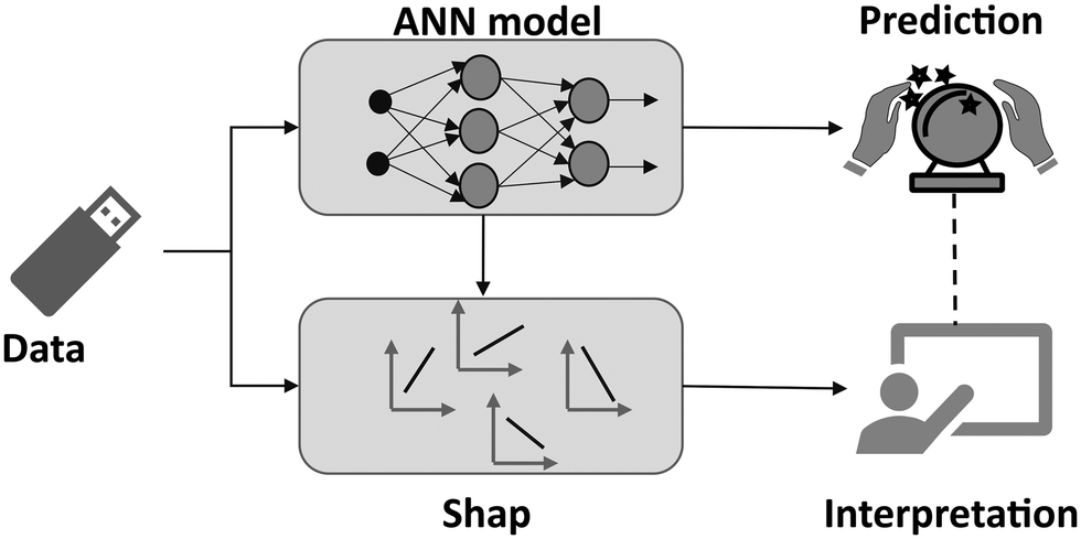
An experimentally validated, single-event microkinetic model developed for the cobalt catalyst based FTS process37 with a single dominant output, methane, is incorporated into a 1-D pseudo-homogeneous plug flow reactor model and is used to in silico generate kinetic data to develop an ANN model. Insights on the decision-making process of the ANN model are obtained with the help of different interpretation techniques such as permutation importance, SHAP value and partial dependence plots. The steps involved in the development of the ANN model and the explanation (interpretation) of results are shown in Fig. 3. The important steps involved in the process are: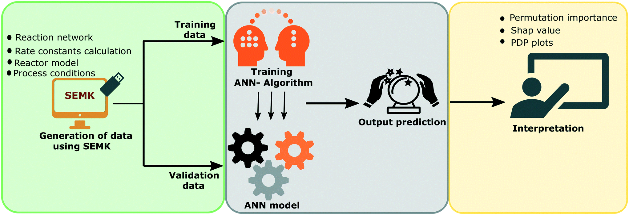 | ||
| Fig. 3 Schematic representation of the different steps involved in ANN model development and interpretation of the model. Data from SEMK simulations (green box) are used for training the ANN model (grey box) which is then analysed using different interpretation techniques (yellow box). | ||
• Step 1: generation of datasets
A dataset comprising 120 data points is generated under the following operating conditions: space-time 9–22 kgcat s molCO−1, syngas molar inlet ratio 3–10 mol mol−1, temperature 483–503 K, and a total pressure of 1.85 bar, as reported by Van Belleghem et al.37 The catalyst and operating conditions in the cited work37 are such that a single dominant output, i.e. methane, is produced. Detailed physicochemical insights on this data from a kinetic model's perspective are discussed in the cited work.37
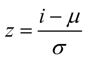
The dataset is split into training and validation datasets with 75 and 45 data points, respectively. The input features used for training the network are space-time (W/FCO), syngas molar inlet ratio (H2/CO) and temperature, with methane yield (YCH4) as output. As the dataset is composed of input features with different units, standardization is performed, where each feature is centered and scaled before training the ANN:
 | (1) |
The validation dataset is then also transformed using μ and σ obtained for the training dataset. Once the scaled datasets have been created, the ANN is trained in the next step.
• Step 2: training and prediction
The scaled input features of the training dataset are fed into the neural network and the model is trained as follows:
1. The weights associated with the neurons are initialized.43
2. Information is shared from one layer to the other to calculate a prediction ŷivia a feed-forward propagation.
3. After the feed-forward propagation step, a loss function is calculated which, in this work, equals the mean square error, MSE (see eqn (2)), based on the methane yield.
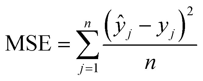 | (2) |
4. The loss function, MSE, is minimised via a back-propagation step. In this step the gradients of the loss function are calculated, and the error is used to update the new weights associated with the neurons.
5. The feed-forward propagation and the back-propagation steps are repeated iteratively (epochs) until the global minimum of the loss function is obtained. In this work, an Adam optimizer44 is used for reaching the global minimum.
6. The final weights associated with the neurons in the network are then used for making predictions using the ANN model.
Once the model is trained, the predictions are made on the so-called validation dataset.
• Step 3: interpretability of the learning process of ANN
The interpretation of the performance of the ANN model developed for FTS is analysed using model agnostic interpretation techniques. The analysis is carried out by investigating the training set using different interpretation techniques such as permutation importance, SHAP value and partial dependence (PD) plots. With the help of permutation importance, the importance of each feature across the entire dataset is obtained. Next, with the help of SHAP values the relevance of each feature in each set of operating conditions is obtained. The combined impact of different input features as interpreted by the developed ANN model is then discussed with the help of partial dependence plots. The steps involved in the calculation of each of these interpretation techniques is further explained in detail below.
1. A neural network model is made using the training dataset containing different input features, and the model error‡ for the training dataset is calculated.
2. To calculate the permutation importance of an input feature (for example, space-time, W/FCO), a new dataset is created by shuffling the rows of that feature in the training dataset (Fig. 4).
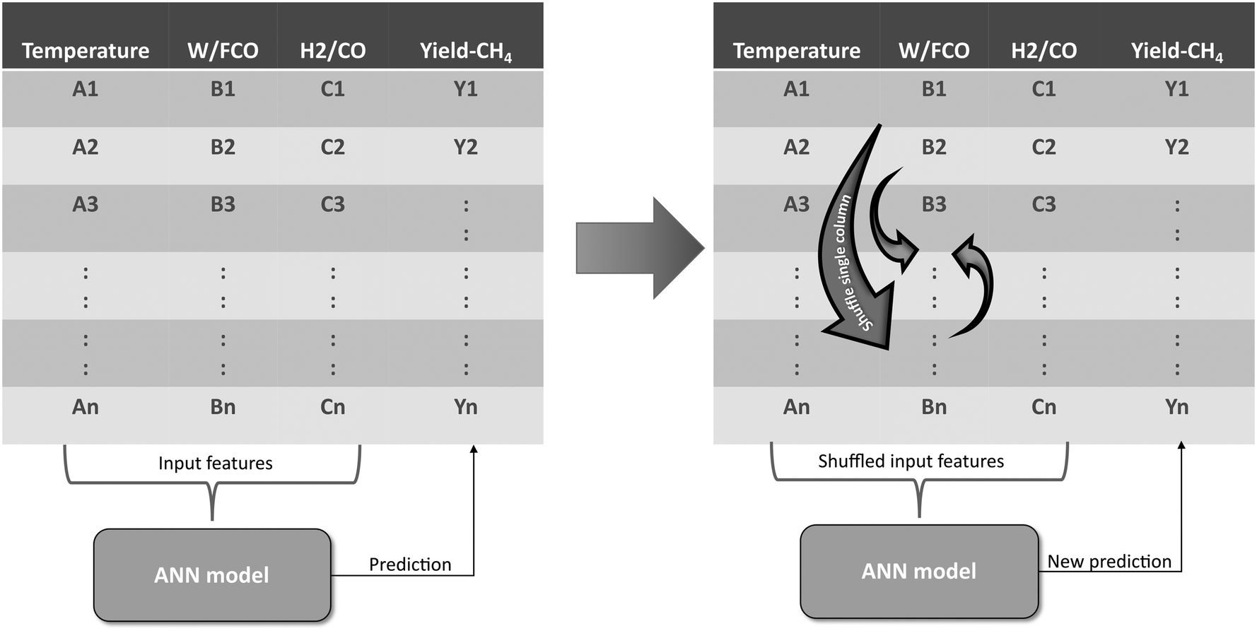 | ||
| Fig. 4 Graphical representation of the permutation importance principle. The model error is calculated using the ANN prediction without permutation (left) and the ANN prediction with permutation (right) of input features such as W/FCO. | ||
3. A prediction for this new dataset is made using the model developed in step 1 above, and the model error is calculated.
4. The permutation importance of the feature is then calculated as the difference of model errors obtained in step 3 and step 1 above.
5. The above steps are repeated for the other input features (i.e. for temperature and syngas molar inlet ratio, H2/CO) to obtain their permutation importance.
The feature resulting in the biggest difference in model error contributes the most to the model prediction, while the feature with the smallest difference contributes the least.
 | ||
| Fig. 5 Graphical representation of how a SHAP model assists in the interpretation of complex ANN models with the help of linear models. | ||
Instead of trying to explain the model in all its complexity, SHAP values focus on how a complex model such as ANN behaves around a single data point. By considering the impact of features on individual data points and then aggregating them, the interplay of combinations of features can be revealed. The SHAP value gives the importance of a feature by comparing the model output obtained with and without that feature. The SHAP value for each feature is calculated as follows:
1. To calculate the SHAP value of a feature i, create all possible subsets of features (SS) from features F, i.e. SS ⊂ F, the feature i being excluded from F. After creating the subsets:
(a) Train a model M(SS1∪i) including the feature i and another model M(SS1) without it, where SS1 is one of the subsets of input features.
(b) Predict the output YM(SS1∪i) with the model M(SS1∪i), using input features in SS1, and the feature i.
(c) Predict the output YM(SS1) with the model M(SS1), using input features in SS1, and calculate the difference from the model prediction including the feature i obtained in step 3.
2. Step 1 is repeated for all possible subsets of input features (without the feature i), i.e. SS1, SS2, SS3, etc., as the effect of excluding the feature i also depends on other input features.
3. The SHAP value (Shapley score) for feature i, ϕi, is then calculated as:
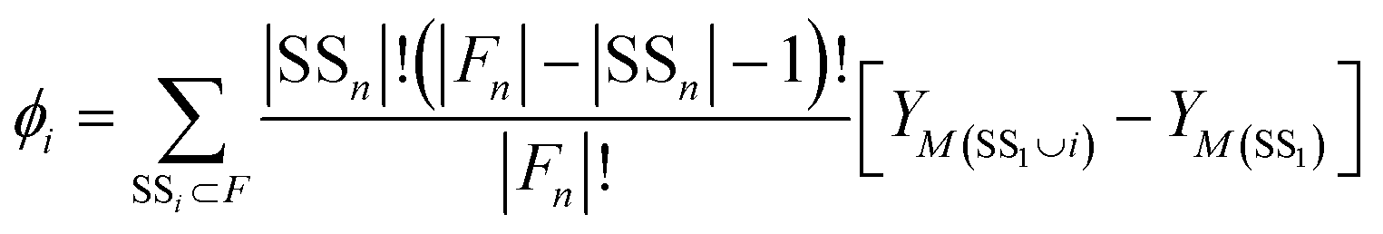 | (3) |
4. Repeat the above steps for all other features to calculate their SHAP values.
The above calculation can be carried out using the SHAP library,46 which calculates SHAP values significantly faster than calculating them via all possible combinations of features.
3 Results and discussion
3.1 Neural network identification and comparison with SEMK
To identify the best performing network, multiple ANN configurations with a different number of neurons and hidden layers were trained using the dataset generated via SEMK simulations. As typically done, sigmoid activation functions are used in the input and output layer, whereas ReLU activation functions are used in the hidden layers, owing to their better performance compared to the other activation function combinations.14The number of hidden layers and neurons in each hidden layer are systematically varied to obtain the best performing model. This is assessed via the parity plot and R2 value. In Fig. 6(a), the variation in the R2 value of the methane yield for the validation dataset is presented as a function of the number of hidden layers and the number of neurons within a hidden layer. A maximum R2 value of 0.99 is obtained using a neural network composed of 3 hidden layers with 20 neurons in each layer. With an increase in the number of neurons, for a fixed number of hidden layers, the R2 value initially increases and attains an optimum value, depending on the number of hidden layers. With a further increase in the number of neurons, the R2 value as calculated against the validation dataset decreases, indicating an over-fitting.
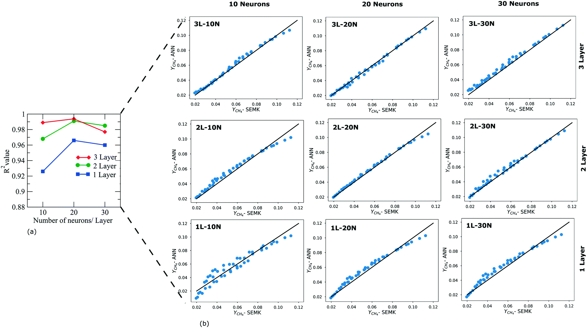 | ||
| Fig. 6 R 2 value (a) and parity diagrams (b) of methane yield obtained with SEMK simulations and ANN predictions when using the validation dataset. Different ANN models with 1–3 hidden layers and 10–30 neurons in each layer are shown. | ||
The neural network configuration that yields the highest R2 value is chosen as the optimal one. Thus, all the analyses reported in this work are carried out using a neural network with 3 hidden layers each containing 20 neurons. This information is more explicit from the parity diagram (Fig. 6(b). From Fig. 7 it is observed that for the optimal neural network configuration, the mean square value of output yield (MSE) for both training and validation datasets converges to a stable value (indicating best learning) after 80 epochs.
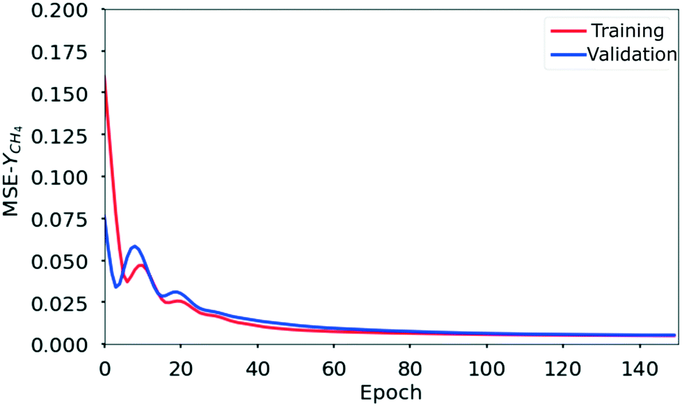 | ||
| Fig. 7 Convergence of the mean square error (MSE) of the methane yield, YCH4 obtained with the ANN model consisting of 3 hidden layers with 20 neurons in each layer. The MSE for the ANN model converges after 80 epochs (iterations). | ||
To show the predictive capability of the ANN, the methane yield (YCH4) obtained with ANN and SEMK simulations are compared in Fig. 8, in which the methane yield is plotted as a function of space-time, at a syngas molar inlet ratio of 10 mol mol−1. It is observed that the methane yield increases with both space-time and temperature. As indicated by the slope of the lines (constant temperature) in Fig. 8, the influence of the space-time on the methane yield increases with temperature. The methane yield obtained at the highest temperature and space-time for a syngas molar inlet ratio of 10 mol mol−1 is about triple that at the lowest temperature and space-time. As the results obtained from SEMK simulations and ANN predictions show a similar trend, it is concluded that the developed ANN model accurately predicts the output generated by the SEMK model in terms of the methane yield.
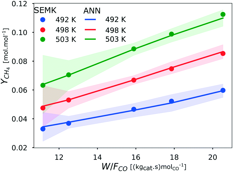 | ||
| Fig. 8 Comparison of the methane yield, YCH4 obtained by SEMK simulations (•) and that with the ANN model (−) as a function of space-time (W/FCO) for varying temperatures at a syngas molar inlet ratio (H2/CO) of 10 mol mol−1. The ANN model consists of 3 hidden layers with 20 neurons in each layer. The 95% confidence limit for the yield obtained with different initializations of the ANN model is represented by the shaded region around the mean ANN prediction (represented by solid line). | ||
3.2 Interpretation of the ANN model
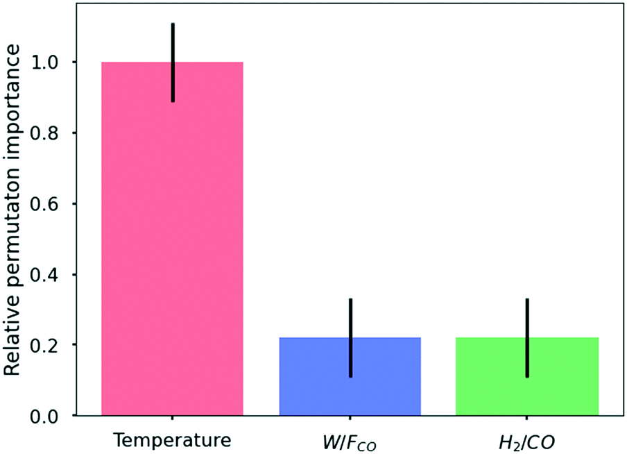 | ||
| Fig. 9 Relative importance of each input feature on a global level (i.e. averaged over the entire range of operating conditions in the training dataset). The relative importance is obtained by scaling the results with that of temperature. The relative importance is calculated using the Python package, Eli5.48 | ||
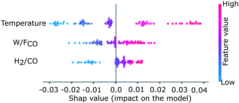 | ||
| Fig. 10 Local interpretation of importance of each input on the training dataset. The local feature importance is quantified in terms of contribution towards yield with respect to the average methane yield obtained from the entire training dataset. The plot is generated using the Python package, SHAP.46 | ||
The combined impact of two input features on the methane yield is shown in Fig. 11. The effect of the 3rd feature is averaged out (by plane averaging the results along the 3rd feature). The combined influence of space-time and temperature is considered in Fig. 11(a). The methane yield increases with an increase of both temperature and space-time. The increase in yield with temperature is more prominent at a higher space-time. The maximum methane yield averaged along the syngas molar inlet ratio (0.11 mol mol−1) is obtained at the highest temperature and the highest space-time. Though the yield increases with space-time at a fixed temperature, the change in yield is less prominent when compared to the change in methane yield with the change in temperature. These observations are in line with the SEMK simulation results reported in Fig. 8. The combined influence of syngas molar inlet ratio and temperature in Fig. 11(b) also indicates the monotonous increase in methane yield with temperature. It is observed that at a lower temperature, the yield is almost unaffected by the syngas molar inlet ratio, while at a higher temperature, the effect of the syngas molar inlet ratio becomes pronounced. From Fig. 11(c), it is observed that at lower space-time the yield is almost unaffected by the syngas molar inlet ratio. However, with an increase in space-time, the dependence of the methane yield on syngas molar inlet ratio increases. From the PD plot analysis it is, however, observed that the maximum yield observed in Fig. 11(a)–(c) varies, depending on the feature importance of the features, whose effect is averaged out in each plot. Although the influence of each feature on the methane yield is determined using the PD plots, it however remains important to check the impact of the averaged feature to confirm the results. This observation is consistent with the nature of these plots, as discussed in section 2.2.3.
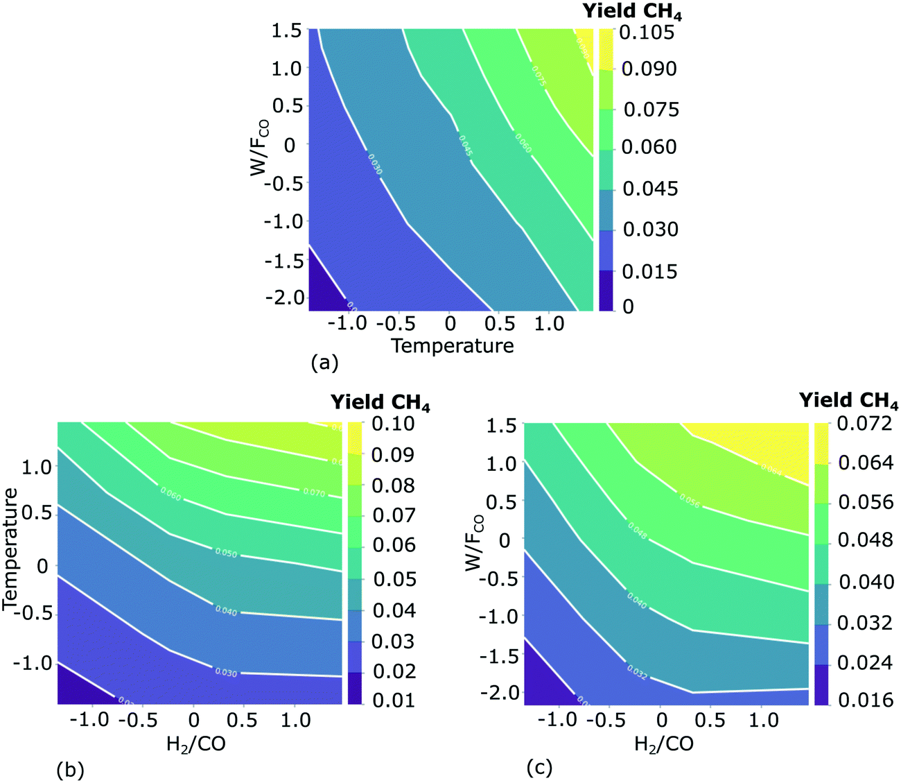 | ||
| Fig. 11 Marginal effect of 2 input features simultaneously considered on the methane yield. The effect of the 3rd feature is averaged out in each subplot, i.e. the results are plane-averaged along the 3rd feature. Effect of space-time (W/FCO) and temperature (a), temperature and syngas molar inlet ratio (H2/CO) (b), and space-time and syngas molar inlet ratio (c) in the range of investigated operating conditions. The input features are standardized for better visualization using the mean and standard deviation of each input feature in the training dataset: temperature (492.8 ± 7.07 K), W/FCO (17 ± 3.5 kgcat s molCO−1), H2/CO (7.4 ± 1.8 mol mol−1). The PD plots are visualized using the Python package, pdpbox.49 | ||
4 Conclusions and perspectives
A machine learning model based on ANN for cobalt-catalysed Fischer–Tropsch synthesis with a single dominant output, methane, is developed using a synthetic dataset generated via a single-event microkinetic (SEMK) model. The optimal ANN model for the FTS process in the investigated range of operating conditions consists of 3 hidden layers with 20 neurons in each layer. This optimal network has an R2 value of 0.99. After confirming that the methane yield obtained with the ANN model represents the one obtained with SEMK simulations, a systematic analysis of the kinetic data is carried out using different interpretation techniques.For the Fischer–Tropsch process, in the range of investigated operating conditions, analysis of the ANN model using interpretation techniques shows that the prominent features follow the order temperature > space-time > syngas molar inlet ratio. The global importance of temperature is roughly 5 times that of space-time and syngas molar inlet ratio. The investigation of the local contribution of each feature (SHAP value) shows a monotonous increase in methane yield with increasing feature values. The coupled impact of input features on the methane yield is observed in the partial dependence plots, with the maximum yield (averaged along the syngas molar inlet ratio) of 0.11 mol mol−1 obtained at the highest temperature and space-time. It is confirmed that analysis of kinetic data can be carried out with the help of an interpretable ANN model. A deeper understanding of the FTS reaction mechanism with the help of these techniques can be achieved using a multi-stage ANN, with process variables as the initial input to predict intermediate outputs such as surface coverages. These coverages can then be fed as an input into the next stage of ANN to predict the performances.
The current work thus shows that more widely applied techniques in data science can now be applied for systematic analysis and interpretation of kinetic data. Similar analysis using experimental data can also help experimenters in their preliminary analysis to detect hidden trends in the data and thus to identify important features. Extensive studies using the different techniques used in this work, for different chemical processes, will also help to identify the most important features. The understanding gained on the decision making by “black-box” ML models such as ANN also enhances the confidence in building hybrid “kinetic ML” models to explain complex chemical processes.
Nomenclature
| F CO | Carbon monoxide molar flow rate at the reactor inlet, mol s−1 |
| H2/CO | Syngas molar inlet ratio, mol mol−1 |
| W/FCO | Space-time, kgcat s molCO−1 |
| Y CH4 | Methane yield, mol mol−1 |
| i | Feature of interest |
| ANN | Artificial neural network |
| F | All input features except feature i of interest |
| FTS | Fischer–Tropsch synthesis |
| ML | Machine learning |
| MSE | Mean square error |
| SEMK | Single-event microkinetics |
| SS | Subset of input features |
| T | Temperature, K |
| W | Catalyst mass, kg |
Conflicts of interest
The authors declare that they have no known competing financial interests or personal relationships that could have appeared to influence the work reported in this paper.Acknowledgements
This work has received funding from the European Regional Development Fund (ERDF) via the PSYCHE project (Interreg France-Wallonie-Vlaanderen) with co-financing from the provinces of East Flanders and West Flanders.Notes and references
- A. Thakkar, S. Johansson, K. Jorner, D. Buttar, J.-L. Reymond and O. Engkvist, React. Chem. Eng., 2021, 6, 27–51 RSC.
- N. S. Eyke, W. H. Green and K. F. Jensen, React. Chem. Eng., 2020, 5, 1963–1972 RSC.
- Y. Yan, T. Mattisson, P. Moldenhauer, E. J. Anthony and P. T. Clough, Chem. Eng. J., 2020, 387, 124072 CrossRef CAS.
- S. Mittal, S. Pathak, H. Dhawan and S. Upadhyayula, Chem. Eng. J., 2021, 413, 127385 CrossRef CAS.
- N. S. Kaveh, F. Mohammadi and S. Ashrafizadeh, Chem. Eng. J., 2009, 147, 161–172 CrossRef.
- F. Kartal and U. Özveren, Energy, 2020, 209, 118457 CrossRef.
- J. Fujima, Y. Tanaka, I. Miyazato, L. Takahashi and K. Takahashi, React. Chem. Eng., 2020, 5, 903–911 RSC.
- C. A. Vandervelden, S. A. Khan, S. L. Scott and B. Peters, React. Chem. Eng., 2020, 5, 77–86 RSC.
- D. S. Palmer, N. M. OBoyle, R. C. Glen and J. B. O. Mitchell, J. Chem. Inf. Model., 2006, 47, 150–158 CrossRef.
- M. H. S. Segler, T. Kogej, C. Tyrchan and M. P. Waller, ACS Cent. Sci., 2017, 4, 120–131 CrossRef.
- P. P. Plehiers, S. H. Symoens, I. Amghizar, G. B. Marin, C. V. Stevens and K. M. V. Geem, Engineering, 2019, 5, 1027–1040 CrossRef CAS.
- J. Athavale, Y. Joshi and M. Yoda, Proceedings of the 17th InterSociety Conference on Thermal and Thermomechanical Phenomena in Electronic Systems, ITherm, 2018, vol. 2018, pp. 871–880 Search PubMed.
- B. C. Csáji, et al., MSc thesis, Faculty of Sciences, Etvs Lornd University, Hungary, 2001, vol. 24, p. 7 Search PubMed.
- D. Graupe, Principles of Artificial Neural Networks, World Scientific, 3rd edn, 2013, vol. 7 Search PubMed.
- M. E. Morocho-Cayamcela, H. Lee and W. Lim, IEEE Access, 2019, 7, 137184–137206 Search PubMed.
- C. Molnar, Interpretable machine learning : a guide for making Black Box Models interpretable, Lulu, Morisville, North Carolina, 2019 Search PubMed.
- L. Breiman, Mach. Learn., 2001, 45, 5–32 CrossRef.
- L. S. Shapley, Proc. Natl. Acad. Sci. U. S. A., 1953, 39, 1095–1100 CrossRef CAS.
- S. Lundberg and S.-I. Lee, 2016, arXiv, 1–6.
- S. M. Lundberg and S. I. Lee, Advances in Neural Information Processing Systems, 2017, 2017-December, pp. 4766–4775 Search PubMed.
- Q. Zhao and T. Hastie, J. Bus. Econ. Stat., 2019, 39, 272–281 CrossRef.
- S. Zhong, K. Zhang, D. Wang and H. Zhang, Chem. Eng. J., 2021, 405, 126627 CrossRef CAS.
- Z. Zhang, M. W. Beck, D. A. Winkler, B. Huang, W. Sibanda and H. Goyal, Ann. Transl. Med., 2018, 6, 216 CrossRef PubMed.
- S. M. Lundberg, B. Nair, M. S. Vavilala, M. Horibe, M. J. Eisses, T. Adams, D. E. Liston, D. K. W. Low, S. F. Newman, J. Kim and S. I. Lee, Nat. Biomed. Eng., 2018, 2, 749–760 CrossRef PubMed.
- S. M. Lundberg, G. Erion, H. Chen, A. DeGrave, J. M. Prutkin, B. Nair, R. Katz, J. Himmelfarb, N. Bansal and S.-I. Lee, Nat. Mach. Intell., 2020, 2, 56–67 CrossRef PubMed.
- S. Tonekaboni, S. Joshi, M. D. McCradden and A. Goldenberg, 2019, arXiv, 1–21.
- D. Brigo, X. Huang, A. Pallavicini and H. S. D. O. Borde, 2021, arXiv, 1–37.
- K. Futagami, Y. Fukazawa, N. Kapoor and T. Kito, J. Finance Data Sci., 2021, 7, 22–44 CrossRef.
- A. Y. Khodakov, W. Chu and P. Fongarland, Chem. Rev., 2007, 107, 1692–1744 CrossRef CAS.
- A. J. Barrios, B. Gu, Y. Luo, D. V. Peron, P. A. Chernavskii, M. Virginie, R. Wojcieszak, J. W. Thybaut, V. V. Ordomsky and A. Y. Khodakov, Appl. Catal., B, 2020, 273, 119028 CrossRef CAS.
- J. Cheng, P. Hu, P. Ellis, S. French, G. Kelly and C. M. Lok, Top. Catal., 2010, 53, 326–337 CrossRef CAS.
- G. Lozano-Blanco, J. W. Thybaut, K. Surla, P. Galtier and G. B. Marin, Ind. Eng. Chem. Res., 2008, 47, 5879–5891 CrossRef CAS.
- C. G. Visconti, E. Tronconi, L. Lietti, R. Zennaro and P. Forzatti, Chem. Eng. Sci., 2007, 62, 5338–5343 CrossRef CAS.
- J. Thybaut and G. Marin, J. Catal., 2013, 308, 352–362 CrossRef CAS.
- G. G. Martens, J. W. Thybaut and G. B. Marin, Ind. Eng. Chem. Res., 2001, 40, 1832–1844 CrossRef CAS.
- W. Feng, E. Vynckier and G. F. Froment, Ind. Eng. Chem. Res., 1993, 32, 2997–3005 CrossRef.
- J. V. Belleghem, C. Ledesma, J. Yang, K. Toch, D. Chen, J. W. Thybaut and G. B. Marin, Appl. Catal., A, 2016, 524, 149–162 CrossRef.
- A. Chakkingal, L. Pirro, A. C. da Cruz, A. J. Barrios, M. Virginie, A. Y. Khodakov and J. W. Thybaut, Chem. Eng. J., 2021, 419, 129633 CrossRef CAS.
- F. A. N. Fernandes, Chem. Eng. Technol., 2006, 29, 449–453 CrossRef CAS.
- H. Adib, R. Haghbakhsh, M. Saidi, M. A. Takassi, F. Sharifi, M. Koolivand, M. R. Rahimpour and S. Keshtkari, J. Nat. Gas Sci. Eng., 2013, 10, 14–24 CrossRef CAS.
- F. A. N. Fernandes, F. E. Linhares-Junior and S. J. M. Cartaxo, Chem. Prod. Process Model., 2014, 9, 97–103 Search PubMed.
- X. Glorot, A. Bordes and Y. Bengio, Proceedings of the fourteenth international conference on artificial intelligence and statistics, 2011, pp. 315–323 Search PubMed.
- J. Guo, AI Notes: Initializing neural networks, https://www.deeplearning.ai/ai-notes/initialization/.
- D. P. Kingma and J. Ba, Adam: A Method for Stochastic Optimization, 2017 Search PubMed.
- A. Fisher, C. Rudin and F. Dominici, J. Mach. Learn. Res., 2019, 20, 177 Search PubMed.
- Welcome to the SHAP documentation, https://shap.readthedocs.io/en/latest/index.html.
- J. H. Friedman, Ann. Stat., 2001, 29, 106834 Search PubMed.
- Overview – ELI5 0.11.0 documentation, https://eli5.readthedocs.io/en/latest/overview.html.
- PDPbox - latest documentation, https://pdpbox.readthedocs.io/en/latest/index.html.
Footnotes |
| † Electronic supplementary information (ESI) available. See DOI: 10.1039/d1re00351h |
| ‡ The model error is the difference between the actual output and the prediction. |
| This journal is © The Royal Society of Chemistry 2022 |