Generating molecules with optimized aqueous solubility using iterative graph translation

Abstract

While molecular discovery is critical for solving many scientific problems, the time and resource costs of experiments make it intractable to fully explore chemical space. Here, we present a generative modeling framework that proposes novel molecules that are 1) based on starting candidate structures and 2) optimized with respect to one or more objectives or constraints. We explore how this framework performs in an applied setting by focusing on the problem of optimizing molecules for aqueous solubility, using an experimental database containing data curated from the literature. The resulting model was capable of improving molecules with a range of starting solubilities. When synthetic feasibility was applied as a secondary optimization constraint (estimated using a combination of synthetic accessibility and retrosynthetic accessibility scores), the model generated synthetically feasible molecules 83.0% of the time (compared with 59.9% of the time without the constraint). To validate model performance experimentally, a set of candidate molecules was translated using the model and the solubilities of the candidate and generated molecules were verified experimentally. We additionally validated model performance via experimental measurements by holding out the top 100 most soluble molecules during training and showing that the model could rediscover 33 of those molecules. To determine the sensitivity of model performance to dataset size, we trained the model on different subsets of the initial training dataset. We found that model performance did not decrease significantly when the model was trained on a random 50% subset of the training data but did decrease when the model was trained on subsets containing only less soluble molecules (i.e., the bottom 50%). Overall, this framework serves as a tool for generating optimized, synthetically feasible molecules that can be applied to a range of problems in chemistry and chemical engineering.

---

Introduction

The discovery of new molecules and materials lies at the heart of many problems in science, ranging from identifying breakthrough cures for infectious diseases to developing technologies to address climate change. Unfortunately, almost every molecular design effort encounters a major, central hurdle: exploring the enormous number of theoretically accessible molecules is cost and time intensive. Traditional molecular design involves using expert chemical knowledge to propose, synthesize, and test new molecules, further limiting the number of molecules that can be reasonably tested.^1,2 Even with an exhaustive experimental search, it has been estimated that only about 10⁸ molecules have ever been synthesized, while the set of potentially synthesizable molecules has been estimated to lie between 10²³ and 10⁶⁰.³

To this end, instead of learning to traverse this vast chemical space, researchers have begun to pursue the inverse molecular design problem:^4,5 that is, given a desired property (or set of properties) f(x), what is the molecule x that will optimize f(x)? In particular, researchers have focused on applying recent advances in deep generative modeling to molecular design.^6–11 One caveat to these studies, however, is that they focus on optimizing properties that can be predicted, such as log P (partition coefficient) or QED (quantitative estimate of drug-likeliness).^12–14 While this provides a convenient way to quickly evaluate properties for large numbers of molecules, it avoids many of the practical challenges associated with applying generative modeling to real applications in chemistry and chemical engineering. Most real molecular design applications involve optimizing properties that are experimentally measured and require synthesizing and experimentally evaluating candidate molecules. Experimental datasets often contain more error and are smaller than datasets calculated computationally. Additionally, in order to test newly generated molecules experimentally, it is necessary to consider their synthetic feasibility.

In this paper, we present a generative modeling framework and explore how this framework performs in an applied setting. Our framework employs graph-to-graph translation, which has been shown to outperform SMILES (simplified molecular input line entry system)-to-SMILES translation models on log P and QED optimization tasks,¹⁵ to translate a given molecular graph into an improved one by providing training pairs of “less optimal” and “more optimal” molecules. Here, we insert a graph-to-graph translation model into an automated workflow where the model is first trained and then used to translate all molecules in the initial dataset. This workflow is then repeated multiple times in order to 1) train a robust translator that can be applied to a given set of candidate molecules for lead optimization and, 2) discover new, highly optimized molecules.

We focus on the problem of designing molecules for high aqueous solubility because this property is critical for a wide variety of chemical applications ranging from geochemistry to drug design. We train our model on a dataset of experimentally obtained aqueous solubility measurements that have non-negligible known experimental error.¹⁶ We then evaluate our model based on its ability to discover novel molecules with high aqueous solubility that are also synthetically feasible. We assess our model's ability to improve candidate molecules in an experimental setting, by measuring the solubility of 3 candidate molecules and 4 molecules that are generated by translating those candidates. We also evaluate our model's ability to generate molecules that are more soluble (based on experimental measurements) than any in the training data by holding out the top 100 most soluble molecules during training. Additionally, to develop an understanding of how our model performs on small datasets, we train our model on multiple subsets of the training data and evaluate its performance. Finally, we explore how chemical structure and properties change during translation and idenfity the types of chemical transformations that the model uses to optimize molecules. In this way, we illustrate how our approach works given the following challenges: 1) training using an experimentally obtained dataset with non-negligible error, 2) constraining the model to generate synthetically feasible molecules, 3) evaluating our model using experimental measurements, and 4) evaluating the sensitivity of model performance to the size of the training dataset. This framework serves as a general approach for generating optimized molecules that can be reapplied to discovering new molecules for a range of applications in chemistry and chemical engineering. Additionally, this work is one of the first examples of training and testing generative modeling in an experimental setting¹⁷ (with one exception¹⁸) and the only work to our knowledge that thoroughly explores the concepts of experimental error, synthetic feasibility, and training dataset size in molecular discovery using generative modeling.

Methods

Dataset preparation

AqSolDB,¹⁶ a publicly available aqueous solubility dataset was used to train the models in this work. This dataset is a compilation of previous databases and contains experimentally obtained measurements that have been estimated to contain an experimental error of approximately 0.5 log S units based on the standard deviations of replicate values (which are only available for a fraction of the dataset).¹⁶ To ensure compatibility between the dataset and each model, we removed any entries containing more than one molecule, any molecules containing unusual/incompatible elements, any invalid SMILES, and the top and bottom 12.5% most and least soluble molecules. After this procedure, 4585 molecules remained and were used for model training.

The graph-to-graph translation model learns to translate a given molecule (referred to as X) into a structurally related molecule with improved solubility (referred to as Y) by learning the relationship between the pairs of molecules, (X,Y), in the training set. The transformation learned by the model depends on how molecules are selected to construct pairs. In this work, we used the pairing algorithm described in Fig. 1a to pair molecules subject to two constraints, 1) molecules must be paired such that their difference in solubility is greater than a threshold value, log S(Y)–log S(X) > α, and 2) molecules must be paired only with structurally similar molecules.

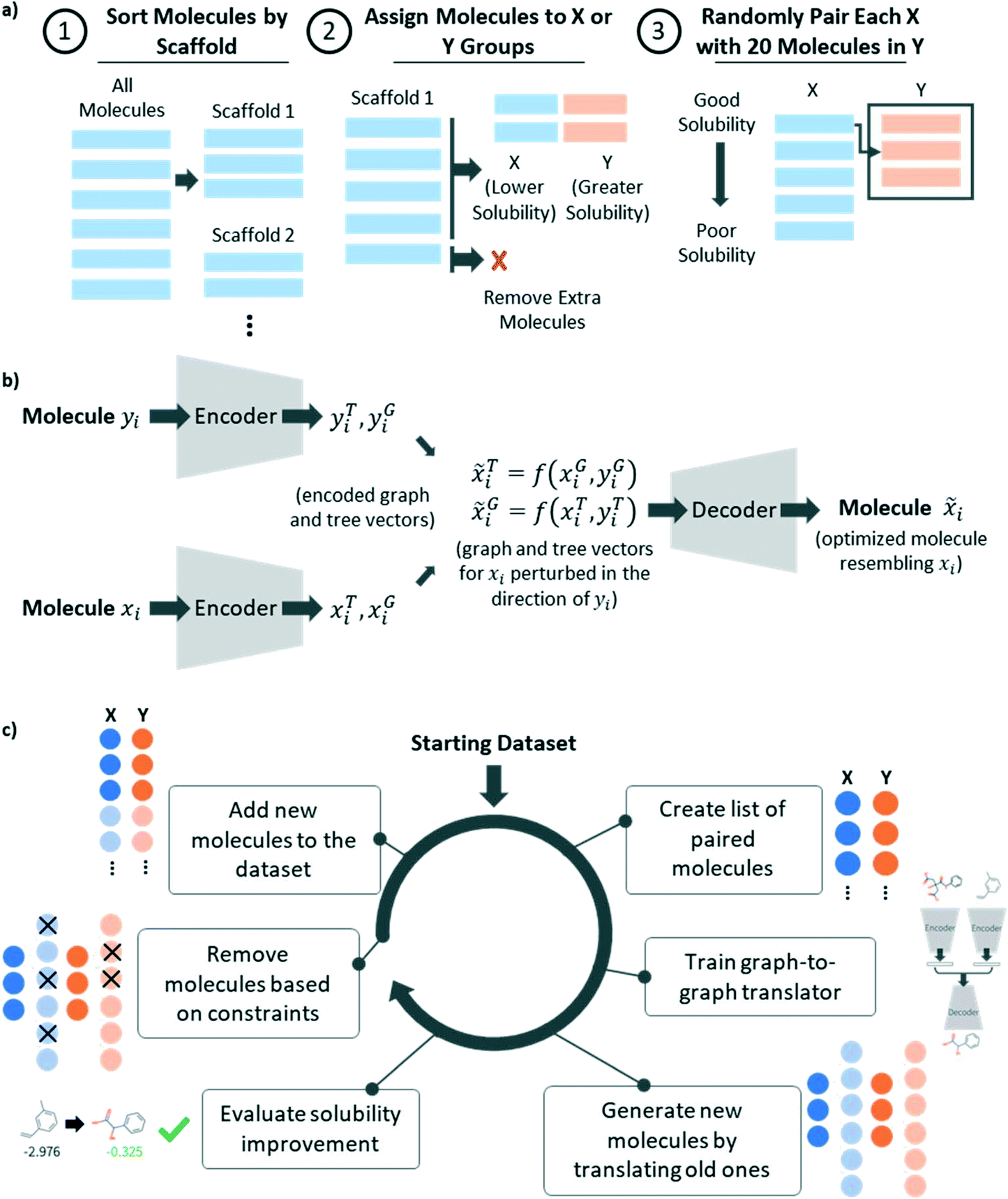Fig. 1 a) Schematic showing the algorithm for creating a list of molecule pairs from a list of labelled molecules. b) Diagram showing the graph-to-graph translator architecture. c) Schematic depicting the operations performed within each training iteration of the graph-to-graph translator.

To achieve these goals, we first grouped molecules that were structurally similar to one another based on whether or not they shared a common scaffold, identified using the Bemis–Murcko algorithm.¹⁹ For all molecules sharing a common scaffold, we assigned molecules with solubility below the median to be X molecules and molecules with solubility above the median to be Y molecules. Any molecules that did not share a scaffold with any other molecules were removed from the dataset. Then, every X molecule was paired randomly with n_pairing different Y molecules, subject to the constraint, log S(Y)–log S(X) > α. Similarly, every Y molecule was paired randomly with n_pairing different X molecules and any duplicate pairs were removed. This process had two hyperparameters, α and n_pairing. α enforces the minimum change in solubility for a given pair and for this work, we set this to be equal to the mean absolute error (MAE) of the predictor model, 0.78, to ensure that all pairs of molecules contained a solubility difference greater than the error in the predictive model. n_pairing determines how many times to pair each molecule and in this work was set to 20. Generally, we observed that pairing with fewer molecules resulted in a smaller training set, reducing model performance, while pairing with a greater number of molecules resulted in overrepresentation of a few highly soluble molecules in the dataset, biasing the learned transformation in the direction of those few molecules. We therefore expect that the choice of this hyperparameter may change for different applications and will be related to the distribution of molecules in the training set.

Graph-to-graph translation

As described previously,^15,22 a graph-to-graph translation model was used to translate less optimal molecules, referred to as X, into more optimal molecules, referred to as Y (shown in Fig. 1b). At training time, the model was provided with a list of paired X and Y molecules, such that all Y molecules were related structurally to X but differed in that they were more soluble. The model used the previously described hierarchical graph encoder,²⁰ involving a molecular-level message passing network (MPN), followed by an attachment-level MPN, followed by a motif-level MPN, to encode each molecule into a latent vector, z_G. The model then calculated a difference vector between the two molecules to characterize the structural differences between molecule X and Y and sample this vector using the reparameterization trick.²¹ The resulting latent code was then recombined with the latent vector corresponding to the X molecule and decoded using the hierarchical graph decoder,²⁰ yielding a molecule resembling the input molecule, X, but perturbed in the direction of the molecule with improved solubility, Y. For greater detail on this method, we refer the reader to prior publications.^15,20 Network architecture details can be found in ESI.†

Iterative graph translation

As described previously,²⁰ the graph-to-graph translator was paired with a predictor in order to iteratively augment the initial training dataset. This augmentation procedure allowed us to train a robust graph-to-graph translation model on a relatively small training dataset. The first step of the iterative procedure, shown in Fig. 1c, was to take the labelled dataset and convert it into a list of pairs. This list of pairs was then used to train the graph-to-graph translator and the resulting model was used to translate every molecule in the initial dataset into a related, more soluble molecule. The resulting translations were then evaluated using the predictor to determine whether they were more soluble. They were also constrained to ensure that each translation was contained with the same Bemis–Murcko scaffold and that each newly generated molecule had a molecular weight above 50 g mol⁻¹. Any molecule resulting from a valid translation was then added to the dataset and any duplicate molecules were removed. The resulting augmented dataset could then be used in the following training cycle. In this work, training was performed for three iterations.

In order to improve the synthetic feasibility of the generated molecules, the model was trained for an additional constrained iteration. Molecules entering the pairing stage of this iteration were removed if they had a synthetic accessibility (SA) score²³ of 3.5 or greater or a retrosynthetic accessibility (RA) score²⁴ of less than 0.8. This constraint was also applied during the translation evaluation phase. The primary improvements made here to the previously published iterative algorithm were 1) an automated approach for pair list generation, 2) addition of pair list generation at the start of every iteration, 3) addition of a molecular weight minimum into the pairing process, and 4) incorporation of an additional synthesizability constraint, based on the synthetic accessibility score and the retrosynthetic accessibility score.

Predictor training

While the dataset used in the first training iteration contains labels obtained from the AqSolDB dataset, a predictor was needed to obtain labels in subsequent generations and to evaluate the solubility of generated models to estimate performance metrics. For this purpose, a directed message passing neural network²⁵ (DMPNN) was trained to predict solubility. Because this model was less sensitive to unusual atom types and outliers, only invalid SMILES and entries containing more than one molecule were removed. The model was trained on 8885 molecules that were randomly split such that 80% of molecules were used in the training set, 10% of molecules were used for validation, and 10% of molecules were used in the test set. The model was trained for 100 epochs using a random split and, as described earlier, the model MAE was 0.78 log S. Architecture and additional performance details can be found in ESI.†

Retrosynthetic tree building using ASKCOS

In order to better qualify the synthetic feasibility of generated molecules, we used ASKCOS²⁶ to generate retrosynthetic pathways for a random subset of molecules for comparison with the SA/RA score measurements. Trees were generated using an expansion time of 240 s, 200 000 templates, and a maximum cumulative template probability of 0.99999. Molecules were considered synthetically feasible if ASKCOS was successful at generating a retrosynthetic pathway within the duration of the expansion time.

Solubility measurement experiments

Materials. Toluene (99.9%), octamethyltrisiloxane (98.0+%), N-methylformamide (99.0+%), dimethyl glutarate (98.0+%), dodecane (99%), N-butoxymethyl acrylamide (96.0+%) were purchased from Fisher and used as received. 2-Heptanone (99%), ethyl formate (97%), methyl butyrate (99%), 4-chlorobutyric acid (99%), 4-fluoroaniline (99%), and pinacolone (97%) were obtained from Sigma Aldrich and used as received. Table S3 in the ESI† shows the source, catalog number, and physical properties for each solvent. Deionized (DI) water was used to prepare the aqueous phase.

Experimental method. Aqueous solutions of each chemical were made by first dispensing water using an air displacement pipette into 1.2 mL vials (Kimble, 60831D-843) on an analytical balance (Mettler AE163). Next, the organic solvent was added using a pipette to reach the desired concentration. The volume of the dispensed fluid was determined by the target mass divided by the solvent density, shown in Table S3.† The vials were then capped with a polyethylene cap.

Once the solutions were made, the vials were put in an 8 × 12 plate and placed in a custom-built phase identification and characterization apparatus (PICA II).²⁷ These formulations were imaged at 20 °C; each vial was removed from the plate by the robot arm, and a digital image was collected. After imaging, the vials were shaken at 695 rpm for 15 s. A second image was captured post-shake. The images were automatically stored in a fully searchable database and indexed according to a specific library identification number, automatically assigned experiment number, and position within the plate. The post-shake images were then analyzed to classify the solution as “soluble” (clear) or “insoluble” (cloudy/phase separated), as shown in Fig. 2.

Fig. 2 Image of a) clear, b) cloudy, and c) phase separated aqueous solutions of 2-heptanone at a) 0.47 wt%, b) 2.9 wt%, and c) 14.9 wt% heptanone. The arrow in c) indicates the phase boundary between the 2-heptanone and water.

Results

Graph-to-graph translator performance

A common challenge with respect to training translation models for property optimization is the sensitivity of the translation to the initial property value of the molecule. To explore this dimension, Fig. 3a–c shows model performance estimated using the DMPNN aqueous solubility predictor (described in Methods) on five evaluation sets that were subsets of the original dataset: the bottom 25 least soluble molecules, 25 molecules near the 25th, 50th, and 75th percentile of the solubility distribution, and the top 25 most soluble molecules. The model was evaluated via three metrics: the average predicted solubility improvement (Fig. 3a), the percentage of translations resulting in solubility improvement (Fig. 3b), and the percentage of translations resulting in an improvement in solubility larger than the MAE of the predictor (Fig. 3c).

Fig. 3 Model performance after 1 (light blue), 2 (medium blue), and 3 (dark blue) iterations based on a) average aqueous solubility improvement, b) percentage of translated molecules that were successfully improved (translated to a molecule with greater solubility), and c) percentage of molecules successfully improved with an improvement greater than the MAE of the DMPNN predictor.

While model performance after a single iteration was relatively good on average (1.02 log S average predicted solubility improvement), model performance was found to be sensitive to the initial solubility of the molecules. One reason for this behavior is the decoder has limited ability to generate molecules that differ significantly from the training data. A second, more heuristic reason for this phenomenon is that for any molecule with a high starting solubility, there may be few valid examples of related molecules with higher solubilities, making the generation problem much more difficult. It is expected that these challenges would exist when applying this approach to other applications and that the extent of model sensitivity would be a function of the nature of the training dataset.

To address these challenges, the graph-to-graph translator was used to augment the initial dataset for three iterations (described in Methods). As shown in Fig. 3a–c, models trained in subsequent iterations performed significantly better than the initial model. In particular, molecules near the 75th percentile of the initial solubility distribution (with an average solubility of −1.75 log S) improved in 87.2% of cases and on average by 0.99 log S units by the third iteration. Molecules in the top 25 of the starting dataset were expected to be challenging to translate because the model was not provided with any examples of molecules with a higher solubility. While after the first iteration, the model on average translated these molecules in the negative direction (indicated by the light blue x on the far right in Fig. 3a), by the third iteration, the model was able to translate these molecules on average in the positive direction 56.4% of the time (Fig. 3b). Thus, by training the graph-to-graph translation model in an iterative workflow, model performance was improved, resulting in successful translations for even the most challenging evaluation sets.

Additional synthesizability objective

A common limitation of many generative models for molecular applications is their tendency to generate molecules that cannot be synthesized in a lab. In this work, the graph-to-graph translator employed a decoder that generates molecules in a motif-by-motif fashion, enforcing that the resulting molecules are generally valid. Despite this, the model can still produce molecules for which there is no synthetic route. While computer aided synthesis planning (CASP) tools can be used to generate a synthetic pathway for a given molecule, thereby suggesting its synthetic feasibility, these approaches are computationally expensive, making them difficult to apply to larger datasets.

Alternatively, a number of scores have been proposed to rapidly (and approximately) evaluate the synthetic feasibility of a given molecule. One score, referred to as the synthetic accessibility (SA) score,^23,28 estimates synthetic feasibility by penalizing molecules containing uncommon structural features and prioritizing molecules containing substructures present in molecules in existing databases including PubChem, ChEMBl, or ZINC. While this approach has been shown to estimate synthetic feasibility reasonably well, its simplistic approach leaves it vulnerable to being tricked by complex molecules containing many reasonable looking fragments or simple molecules containing uncommon fragments.²⁹ An alternative score, referred to as the retrosynthetic accessibility (RA) score,²⁴ instead estimates synthetic feasibility using a machine learned model trained on predictions from a CASP model (AiZynthFinder). Importantly, this model consists of a deep neural network that uses the full molecular structure as an input, allowing it to learn a more nuanced definition of synthetic feasibility. One caveat to the RA score, however, is that it directly relies on a CASP model and therefore any shortcomings of that model will also be present in the RA score.

In this study, we evaluate the synthetic feasibility of our generated molecules using a combination of the SA and RA scores, where molecules that have SA score < 3.5 and RA score > 0.8 are taken to be synthetically feasible (thresholds were estimated based on the scores corresponding to molecules in the training data). Fig. 4a shows the distribution of the SA and RA scores of the initial training data, divided into four quadrants. As expected, most of the training data (86.7%) are considered synthetically feasible with respect to both scores, while only a small subset of the data (3.6%) is considered synthetically infeasible by both scores. Additional small subsets of the training data (3.6% and 6.1%) are considered feasible by only one of the two scores.

Fig. 4 Joint distribution of the SA and RA synthetic feasibility scores for a) the initial training dataset, b) the dataset after three iterations, and c) the dataset after three iterations of training followed by an additional iteration with the SA and RA scores constrained. Model performance after three iterations (blue) and after the constrained iteration (orange) based on d) average aqueous solubility improvement, e) percentage of translated molecules that were successfully improved (translated to a molecule with greater solubility), and f) percentage of molecules successfully improved with an improvement greater than the MAE of the DMPNN predictor.

Fig. 4b shows the distribution of the SA and RA scores of the generated molecules after three iterations of training. While the number of unique molecules in our dataset grew from 4585 molecules in the initial training dataset to 127 094 molecules after the third iteration, only 59.9% of those molecules were synthetically feasible with respect to both the SA and RA scores (Fig. 4b, lower-right quadrant). To address this challenge, we performed an additional, constrained iteration of model training by removing any molecules with SA score > 3.5 and RA score < 0.8 from the dataset (described in Methods). This reduced the number of unique molecules to 64 795 used for training in the constrained iteration. As shown in Fig. 4c, after the constrained iteration, the dataset (now 176 321 unique molecules) contained 83.0% feasible molecules and 3.4% infeasible molecules (evaluated with respect to both scores). 8.1% of molecules had a good RA score but a poor SA score and 5.5% of molecules had a good SA score but a poor RA score. In this way, performing an additional constrained iteration achieves similar SA and RA score distributions (when compared with the initial training data). Examples of molecules in each quadrant are shown in Fig. 5.

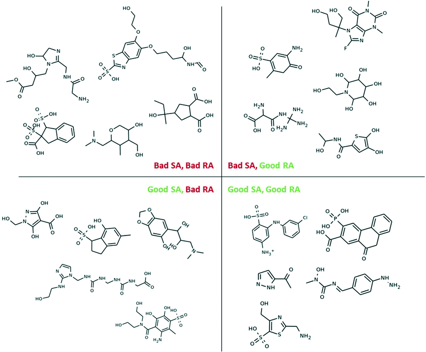Fig. 5 Examples of molecules with good and bad SA and RA scores.

Even after constraining the model, a non-negligible subset (13.6%) of molecules in the dataset only satisfy the synthetic feasibility constraints with respect to one of the scores (Fig. 4c). Additionally, as described earlier, both scores have been shown to fail under different circumstances when estimating synthetic feasibility.^24,29 To explore the robustness of our approach, we randomly selected 100 molecules from each of the four quadrants in the final dataset and used a CASP model called ASKCOS²⁶ to predict retrosynthetic routes. While ASKCOS (or any CASP model) is not a true determinant of which molecules are synthetically feasible, it does offer an automated, conservative metric. Importantly, we chose a different CASP model than the one used to develop the RA score to ensure that our three approaches to measuring synthetic feasibility were independent. We found that with an expansion time of 4 minutes, ASKCOS was able to identify retrosynthetic trees for 46 of the 100 molecules with both good SA and good RA scores, 12 molecules with good SA and bad RA scores, 9 molecules with good RA and bad SA scores, and 2 molecules with bad SA and RA scores (additional details can be found in ESI†). In this way, although ASKCOS offers a more conservative view of synthetic feasibility, it is more likely to identify synthetic pathways for molecules with both good SA and RA scores. We note that it is likely that a larger number of retrosynthetic trees would be found with a larger expansion time.

In addition to evaluating the effectiveness of the SA/RA score constraints in improving synthetic feasibility it is important to quantify the effect of this constraint on model performance. As shown in Fig. 4d–f, the model achieved equal or better performance after the constrained iteration (orange) compared with model performance after only three iterations (blue). This trend was consistent across each method of measuring improvement: average solubility improvement, percent improved, and percent improved past the MAE of the predictive model. This illustrates that introducing synthetic feasibility score-based constraints is a good strategy for generating optimized, synthetically feasible molecules.

Discovering novel, optimized molecules

In addition to using iterative augmentation to improve model performance and incorporate secondary objectives, this approach can be used as a method to search for novel, optimized molecules. After augmenting the training dataset for three iterations, the dataset grew from 65 310 training pairs consisting of 4585 unique molecules to ∼2 million training pairs consisting of ∼120 000 unique molecules (Fig. 6a and b, respectively). Some of the molecules added in subsequent iterations had solubilities that were predicted to be greater than any of the molecules in the original dataset. Fig. 6e shows the predicted solubilities for the top ten molecules in the dataset at the end of each iteration. After each iteration, the predicted solubilities for the top ten molecules increased such that, by the third iteration, all ten molecules had greater solubilities than any of the original top ten molecules by a margin greater than 1 log S unit.

Fig. 6 a) Number of training pairs after each iteration. b) Number of unique molecules after each training iteration. c) Diversity and d) novelty of generated molecules after each iteration. e) Aqueous solubility of top ten molecules at the end of each iteration. f) Solubility distribution of top 100 molecules (light grey) and 33 re-discovered molecules (dark grey).

When searching for optimized molecules, it is often desirable to generate molecules that are diverse and novel. Here, we define diversity as:

where N is the number of generated molecules and Tanimoto refers to the Tanimoto similarity between molecules (computed using Morgan fingerprints). We define novelty as the percentage of generated molecules that have improved solubility and have a Tanimoto similarity of less than 0.4 with respect to their parent molecule, as has been done previously.^10,17 Since diversity and novelty depend on the molecules included in the translated dataset, we assessed each metric with respect to the previously defined evaluation sets. The diversity of molecules generated from the different evaluation sets ranged from 0.83 to 0.93 and the novelty from 0.79 to 0.98 (Fig. 6c and d). While we observe no clear trend in the novelty of generated molecules, we do observe that the diversity of generated molecules drops slightly after the final, constrained iteration. This may be because introducing additional constraints to the generator limits the types of molecules that can be generated, as has been seen previously.³⁰

While we expect that the diversity and novelty of molecules generated using this approach will be somewhat application specific, we note that our model's performance with respect to these metrics is in the same range as the equivalent metrics for other recently reported generative models.³¹

Hold-out experiment

One possible caveat to these results is that the solubility for each newly generated molecule is predicted using a trained DMPNN model (described in Methods). Thus, it is possible that the top ten molecules shown in Fig. 6e are not more soluble but are instead poorly predicted by the DMPNN model. To address this concern, we trained the model for three iterations while withholding the top 100 molecules in the original dataset. As shown in Fig. 6f, after three iterations, the model re-discovered 33 of the 100 original molecules. The most soluble molecule for which there was experimental data had a solubility of 1.58 log S and was 0.52 log S more soluble than the most soluble molecule provided to the model during training. This experiment can be thought of as providing a lower bound for this approach's ability to optimize solubility.

Model performance on smaller datasets

For many applications, a common difficulty with using deep generative models to design optimized molecules is the lack of a sufficiently large dataset to accurately train a deep neural network. While the AqSol database provides a large number of molecules and their experimentally measured solubilities, it would be valuable to be able to optimize molecules for properties for which there are fewer data. To evaluate how the model performs on smaller datasets, the model was trained on a range of subsampled datasets representing either a random part or the bottom part of the distribution. Evaluating the model on random subsets of the distribution illustrates how model performance changes with the number of training data while evaluating the model on subsets representing the bottom x% of the distribution illustrates how the model performs for the specific case where the starting dataset is both smaller and farther from the theoretical optimum. The subsampled datasets tested in this study were a random 10%, 20%, and 50% of the distribution (Fig. 7a) and the bottom 20% and 50% of the distribution (Fig. 7b). In order to study the sensitivity of the generator independent of the predictor, we did not retrain the predictor on the smaller datasets, but rather used the predictor that was previously trained on the full dataset (described in Methods). Note: subsampling was performed before dataset cleaning and pairing and, as a result, the percent reduction in dataset size was not exact.

Fig. 7 a) and b) Solubility distribution for the randomly subsampled datasets and bottom subsampled datasets, respectively. c) Number of unique molecules (top) and number of training pairs (bottom) after each iteration. d) and e) Model performance with respect to average solubility improvement, percent improvement, and percent of molecules successfully improved with an improvement greater than the MAE of the DMPNN predictor. f) Solubility of top ten molecules for each subsampled dataset and the full dataset after each iteration.

Fig. 7d and e shows the performance of the model trained for three iterations on each of the subsampled datasets relative to the full dataset. The model performed significantly worse when trained on any dataset comprising the bottom part of the distribution (shown in red) compared to random subsets of the distribution (shown in green). The model trained on the 50% randomly subsampled dataset (2110 molecules) performed as well as the model trained on the full dataset across all three metrics. The models trained on the 20% and 10% randomly subsampled datasets (818 and 495 molecules, respectively) performed worse than the model trained on the original dataset, but still better than the model trained on the bottom 50% or 20% of the data (1734 molecules and 583 molecules, respectively). This illustrates that the performance of the translator is less sensitive to dataset size and is more sensitive to the dataset distribution.

While the performance of the translator function of the model is fairly insensitive to dataset size, the ability of the model to discover new, highly soluble molecules is more sensitive. Fig. 7f shows the solubilities of the top 10 molecules discovered after three iterations by models trained on each subset of the dataset. The solubilities of the most soluble molecules increased considerably with the size of each dataset and the top ten molecules discovered by the model trained on the full dataset are all more soluble than any of the molecules discovered on any model trained on any subset.

Model evaluation in an experimental workflow

While we have shown that our model can discover molecules that have greater predicted aqueous solubility, it is valuable to experimentally probe whether our approach can be used to translate less soluble “parent” molecules into more soluble molecules that are not present in the training data. To generate molecules to test experimentally, 4 parent molecules, toluene, dodecane, 2-heptanone, and octamethyltrisiloxane, were translated 1000 times each, yielding 2982 unique molecules. This set of molecules was then restricted to molecules that were liquid at room temperature and had minimal handling challenges. Importantly, to eliminate the need for synthesizing new molecules, we limited our study to molecules that could be purchased. Considering these criteria, we selected 8 molecules (listed in Table 1) for experimental validation such that the predicted solubilities of these molecules would cover the entire solubility distribution in log S. The experimental set also incorporated five additional molecules that were present in the AqSolDB training dataset (marked with * in Table 1) to facilitate comparisons between experimental results, training data and modeling predictions.

Table 1 The parent molecules and down-selected generated molecules for the experimental workflow. Molecules in bold represents the parent molecules. * denotes the molecules that are present in the original AqSol training dataset

Selected molecules	Predicted solubility (log S, mol L^−1)	AqSolDB data (log S, mol L^−1)	Experimental solubility (wt%)		Experimental solubility (log S, mol L^−1)
			Low end	High end	Low end	High end
Toluene*	−1.80	−2.21	0.1%	0.4%	−1.85	−1.33
4-Fluoroaniline*	−0.34	−0.53	1.0%	2.8%	−1.06	−0.59
Dodecane	−7.02	—	—	0.2%	—	−1.98
Methyl butyrate*	−0.71	−0.83	1.1%	3.6%	−0.95	−0.45
4-Chlorobutyric acid	0.09	—	13.8%	32.2%	0.06	0.45
2-Heptanone	−1.25	—	0.5%	0.9%	−1.39	−1.10
N-Butoxymethyl acrylamide*	−0.44	−0.65	1.0%	3.0%	−1.21	−0.72
Ethyl formate	0.25	—	7.1%	14.9%	−0.02	0.30
Octamethyltrisiloxane	−6.83	—	—	0.2%	—	−2.11
Pinacolone*	−1.58	−0.72	0.4%	0.9%	−1.37	−1.05
Dimethyl glutarate	−0.37	—	2.9%	6.5%	−0.74	−0.39
N-Methylformamide	1.20	—	94.9%	—	1.21	—

---

Solubilities of the 12 molecules (4 parent + 8 generated) were experimentally measured by formulating aqueous solutions at target solute concentrations of 0.2, 0.5, 1, 3, 7, 15, 34 and 95 wt% respectively. Cloudiness of each solution was determined by image analysis and assigned as clear (soluble) or cloudy/separated (insoluble) (further details can be found in ESI†). Using this analysis, “Low End” (Table 1) represents the highest concentration for which the solution appeared clear and the “High End” represents the lowest concentration for which the solution appeared cloudy. To compare the experimentally measured solubility of the molecules with the predicted values in mol L⁻¹, we converted the concentration in wt% to mol L⁻¹ by neglecting the volume change during mixing between water and solute molecules. We note that the assumption of ideal mixing does not hold especially at high concentrations, however, the deviation is not significant for solubility comparisons at log scale as even a 10% volume change in mixing only alters solubility by 0.046 (log(0.9)) in log S.

For validation of our experimental method, solubilities of the five molecules that existed in the AqSol training set are presented in Fig. 8a. The solubility discrepancy between the AqSol data and the predicted solubility ranges from 0.12–0.86 in log S. In comparison, a majority of the experimentally measured solubility ranges either overlap or are extremely close to the AqSol database result. Sorkun et al.¹⁶ describe that the approximate average standard deviation in the AqSol database is roughly 0.50 in log S; herein, the experimental error in solubility measurement should also be considered. For example, in our experiments, the chemicals were used as received and thus may have affected the experimental result due to the presence of impurities and residual moisture in the chemical. Additionally, the ambient temperature can also play a role in slight differences in solubility. Given that the discrepancy between the experimental result and the database value is not higher than the MAE of the model (0.78 in log S) nor the estimated deviation in the AqSol dataset (∼0.5), the experimental method was found to be sufficiently robust to validate our generative model.

Fig. 8 Experimentally determined solubility (shaded boxes) overlaid with model predicted solubility (green diamonds) and AqSol database data (blue triangles, if applicable) for (a) molecules present in the AqSol data set and (b) unique molecules from the model.

Fig. 8b illustrates the predicted and experimental solubility for the newly generated molecules (not present in the AqSol dataset). In each case, the generated molecules were shown to have solubility ranges that were greater than (and non-overlapping with) the parent molecules. This illustrates that our translation model can generate molecules that are not only predicted to be more soluble, but also are experimentally shown to be more soluble.

A closer look at how the model translates molecules

Often, chemists add or change chemical groups on a molecule in order to improve its solubility. This leads to the question: how does our model learn to translate less soluble molecules into more soluble molecules, and how does this compare with our chemical intuition? To study this process, Fig. 9a–c shows how the probabilities of observing three common chemical moieties, hydroxyl, thiol, and sulfate groups, change with translation after each iteration of model training. As was done previously, statistics are reported with respect to the five evaluation sets with increasing starting solubilities.

Fig. 9 The probability of finding a a) hydroxyl, b) thiol, or c) sulfate group in the reference evaluation set (black) and generated molecules after 1 (light blue), 2 (medium blue), and 3 (dark blue) iterations. d) Top: The average molecular weight of the reference evaluation set (black) and generated molecules after 1 (light blue), 2 (medium blue), and 3 (dark blue) iterations. Bottom: The distribution of the molecular weight of the reference evaluation set and the molecules generated after iteration 3.

On average, after one iteration, the model learned to leverage adding hydroxyl groups and removing thiol groups in order to increase the solubility of input molecules. Interestingly, in subsequent iterations, the model relied more on these chemical groups, adding hydroxyl groups and removing thiol groups with greater frequency. Similarly, the model learned to use sulfate groups to increase the solubility of molecules but, because sulfate groups were less common in the starting dataset, it took multiple iterations for the model to consistently leverage this chemical moiety. In fact, even by the third iteration, the model on average translated the top 25 evaluation set to a set of molecules with fewer sulfate groups. Thus, it appears that by training the model on an augmented dataset, the model is able to learn increasingly about how specific chemical groups can be used to improve solubility.

Another common approach for changing a molecule to make it more soluble is reducing its molecular weight. Fig. 9d shows the average molecular weight of molecules translated by the model after each iteration. Despite the fact that the model on average improved solubility to a greater degree in every subsequent iteration, the average molecular weight of the translated molecule increased after every iteration. This is contrary to what would be expected and suggests that after each iteration the model better learns how to balance the tradeoff between molecular weight and addition of highly soluble chemical groups. We note that, as described earlier, to avoid the model translating molecules into small molecules that were likely to be gases at room temperature, we imposed a lower bound on the molecular weight of translated molecules of 50 g mol⁻¹.

To illustrate these phenomena, we show an example of a translation of an input molecule, N-(4-bromo-2-methylphenyl)acetamide, based on the model after three iterations in Fig. 10. As can be seen in the figure, instead of reducing the size of this molecule, the model adds on additional chemical groups including carboxylates, sulfates, hydroxyl groups, and others. Thus, each of the translated molecules has a higher molecular weight than the starting molecule. The addition of these groups while also trying to minimize molecular weight often results in unusual molecules that cannot be synthesized (or at least not easily). Thus, it is useful to include synthetic feasibility as an additional constraint in order to guide the model toward feasible, optimized molecules.

Fig. 10 Example translation of N-(4-bromo-2-methylphenyl)acetamide into related, but more soluble molecules by the model after three iterations of training. The model tends to add additional hydrophilic groups to the molecule as opposed to reducing the molecules size. We note that these molecules were generated by the model trained without the synthesizability constraint.

Conclusions

In this work, we used a graph-to-graph translator in an iterative framework to optimize molecules for aqueous solubility. We first demonstrated the model's ability to translate a given candidate molecule into a related, more soluble molecule and found that model performance was better for molecules with lower starting solubilities and worse for molecules with higher starting solubilities. Despite this, model performance improved after multiple iterations of training, independent of starting solubility. We then introduced a synthetic feasibility constraint based on synthetic accessibility (SA) and retrosynthetic accessibility (RA) scores and improved the probability of generating synthetically feasible molecules from 59.9% to 83.0%. We also found that the model was able to generate novel and diverse molecules after each iteration of training and that some of these molecules had solubilities greater than any of the molecules in the training dataset. We then investigated the sensitivity of model performance to dataset size by training the model on different subsets of the initial training dataset and found that model performance did not decrease significantly when the model was trained on a random 50% subset of the training data but did decrease when the model was trained on subsets with less soluble molecules. Model performance was then validated experimentally by using the model to translate a set of candidate molecules and determining the solubilities of the candidate and generated molecules experimentally. Finally, we explored the logic the model uses to improve solubility by studying how chemical groups and properties change before and after translation. Overall, this framework offers an approach to generate optimized, synthetically feasible molecules that can be broadly applied to a range of chemical applications, including applications with limited dataset sizes.

Conflicts of interest

There are no conflicts of interest to declare. Professor Barzilay is currently serving as a SAB member for Amgen Data Science, Janssen, and Immunai and as a BOD member for Dewpoint Therapeutics.

Acknowledgements

The authors gratefully acknowledge discussions with Esther Heid. This work was funded by Dow under the University Partnership Initiative (#252048AF). The authors thank Dow, DARPA (HR00111920025), the Abdul Latif Jameel Clinic for Machine Learning in Health, the DTRA Discover of Medicinal Countermeasures Against New and Emerging (DOMANE) threats program, and the consortium Machine Learning for Pharmaceutical Discovery and Synthesis (http://mlpds.mit.edu) for support.

References

1. C. W. Coley, N. S. Eyke and K. F. Jensen, Angew. Chem., Int. Ed., 2020, 59, 22858–22893.
2. C. W. Coley, Trends Chem., 2020, 3, 133–145.
3. J.-L. Reymond and M. Awale, ACS Chem. Neurosci., 2012, 3, 649–657.
4. D. Xue, Y. Gong, Z. Yang, G. Chuai, S. Qu, A. Shen, J. Yu and Q. Liu, WIREs Comput. Mol. Sci., 2019, 9, e1395.
5. B. Sanchez-Lengeling and A. Aspuru-Guzik, Science, 2018, 361, 360–365.
6. R. Gómez-Bombarelli, J. N. Wei, D. Duvenaud, J. M. Hernández-Lobato, B. Sánchez-Lengeling, D. Sheberla, J. Aguilera-Iparraguirre, T. D. Hirzel, R. P. Adams and A. Aspuru-Guzik, ACS Cent. Sci., 2018, 4, 268–276.
7. D. H. Brookes and J. Listgarten, Design by Adaptive Sampling, 2020, arXiv:1810.03714.
8. R.-R. Griffiths and J. M. Hernández-Lobato, Chem. Sci., 2020, 11, 577–586.
9. Q. Liu, M. Allamanis, M. Brockschmidt and A. Gaunt, 2019, arXiv:1805.09076.
10. M. Olivecrona, T. Blaschke, O. Engkvist and H. Chen, J. Cheminformatics, 2017, 9, 48,  DOI:10.1186/s13321-017-0235-x.
11. M. Popova, O. Isayev and A. Tropsha, Sci. Adv., 2018, 9(1), 48,  DOI:10.1126/sciadv.aap7885.
12. G. R. Bickerton, G. V. Paolini, J. Besnard, S. Muresan and A. L. Hopkins, Nat. Chem., 2012, 4, 90–98.
13. A. Grosnit, et al., 2021, arXiv:2106.03609.
14. A. Tripp, E. Daxberger and J. M. Hernández-Lobato, NeurIPS, 2020.
15. W. Jin, K. Yang, R. Barzilay and T. Jaakkola, ICLR, 2019.
16. M. C. Sorkun, A. Khetan and S. Er, Sci. Data, 2019, 6, 143,  DOI:10.1038/s41597-019-0151-1.
17. A. R. Thawani and R. Griffiths, et al., ICLR, 2020.
18. A. Zhavoronkov, Nat. Biotechnol., 2019, 37, 1038–1040.
19. G. W. Bemis and M. A. Murcko, J. Med. Chem., 1996, 39, 2887–2893.
20. W. Jin, R. Barzilay and T. Jaakkola, ICML, 2020.
21. D. P. Kingma and M. Welling, 2014, arXiv:1312.6114.
22. K. Yang, W. Jin, K. Swanson, R. Barzilay and T. Jaakkola, 2020, arXiv:2002.04720.
23. P. Ertl and A. Schuffenhauer, J. Cheminformatics, 2009, 1, 8,  DOI:10.1186/1758-2946-1-8.
24. A. Thakkar, Chem. Sci., 2021, 12, 3339–3349.
25. K. Yang, K. Swanson, W. Jin, C. Coley, P. Eiden, H. Gao, A. Guzman-Perez, T. Hopper, B. Kelley, M. Mathea, A. Palmer, V. Settels, T. Jaakkola, K. Jensen and R. Barzilay, J. Chem. Inf. Model., 2019, 59, 3370–3388.
26. C. W. Coley, D. A. Thomas, J. A. M. Lummiss, J. N. Jaworski, C. P. Breen, V. Schultz, T. Hart, J. S. Fishman, L. Rogers, H. Gao, R. W. Hicklin, P. P. Plehiers, J. Byington, J. S. Piotti, W. H. Green, A. J. Hart, T. F. Jamison and K. F. Jensen, Science, 2019, 365,  DOI:10.1126/science.aax1566.
27. C. E. Mohler, R. L. Kuhlman, C. A. Witham and M. K. Poindexter, AADE, 2011, p. 11.
28. Y. Fukunishi, T. Kurosawa, Y. Mikami and H. Nakamura, J. Chem. Inf. Model., 2014, 54, 3259–3267.
29. W. Gao and C. W. Coley, J. Chem. Inf. Model., 2020, 60, 5714–5723.
30. Y. Li, L. Zhang and Z. J. Liu, ChemInform, 2018, 10, 33,  DOI:10.1186/s13321-018-0287-6.
31. B. Chen, T. Wang, C. Li, H. Dai and L. Song, ICLR, 2021.

---

Footnote

† Electronic supplementary information (ESI) available: Architecture and training details for the hierarchical graph neural network (HGNN) and the directed message passing neural network (DMPNN), details regarding the experimental approach used for quantifying aqueous solubility, examples of molecules with good/bad SA/RA scores, and details on representative molecules used in ASKCOS retrosynthesis. See DOI: 10.1039/d1re00315a

---