
 Open Access Article
 This Open Access Article is licensed under a
 Creative Commons Attribution 3.0 Unported Licence
Apples to apples comparison of standardized to unstandardized principal component analysis of methods that assign partial atomic charges in molecules
Thomas A. Manz *
*
Chemical & Materials Engineering, New Mexico State University, Las Cruces, New Mexico 88003-3805, USA. E-mail: tmanz@nmsu.edu
First published on 3rd November 2022
Abstract
Articles by Cho et al. (ChemPhysChem, 2020, 21, 688–696) and Manz (RSC Adv., 2020, 10, 44121–44148) performed unstandardized and standardized, respectively, principal component analysis (PCA) to study atomic charge assignment methods for molecular systems. Both articles used subsets of atomic charges computed by Cho et al.; however, the data subsets employed were not strictly identical. Herein, an element by element analysis of this dataset is first performed to compare the spread of charge values across individual chemical elements and charge assignment methods. This reveals an underlying problem with the reported Becke partial atomic charges in this dataset. Due to their unphysical values, these Becke charges were not included in the subsequent PCA. Standardized and unstandardized PCA are performed across two datasets: (i) 19 charge assignment methods having a complete basis set limit and (ii) all 25 charge assignment methods (excluding Becke) for which Cho et al. computed atomic charges. The dataset contained ∼2000 molecules having a total of 29![[thin space (1/6-em)]](https://www.rsc.org/images/entities/char_2009.gif) 907 atoms in materials. The following five methods (listed here in alphabetical order) showed the greatest correlation to the first principal component in standardized and unstandardized PCA: DDEC6, Hirshfeld-I, ISA, MBIS, and MBSBickelhaupt (note: MBSBickelhaupt does not appear in the 19 methods dataset). For standardized PCA, the DDEC6 method ranked first followed closely by MBIS. For unstandardized PCA, Hirshfeld-I (19 methods) or MBSBickelhaupt (25 methods) ranked first followed by DDEC6 in second place (both 19 and 25 methods).
907 atoms in materials. The following five methods (listed here in alphabetical order) showed the greatest correlation to the first principal component in standardized and unstandardized PCA: DDEC6, Hirshfeld-I, ISA, MBIS, and MBSBickelhaupt (note: MBSBickelhaupt does not appear in the 19 methods dataset). For standardized PCA, the DDEC6 method ranked first followed closely by MBIS. For unstandardized PCA, Hirshfeld-I (19 methods) or MBSBickelhaupt (25 methods) ranked first followed by DDEC6 in second place (both 19 and 25 methods).
1. Introduction
Many factors should be considered when assessing the performance of methods for assigning partial atomic charges.1–3 Six factors that bear special consideration here include the following:(1) The method should have a well-defined mathematical limit as the basis set is improved towards completeness (aka ‘a complete basis set limit’) and have atomic charge values that do not depend on the orientation of the external coordinate system (aka ‘rotational invariance’).3
(2) An assigned atomic charge should correspond to assigning some non-negative number of electrons to the atom. This means the assigned atomic charge should not exceed the atom's atomic number.
(3) Ideally, the method should work reliably across diverse material types including those containing both surface and buried atoms.
(4) The assigned atomic charges should exhibit similar values across similar chemical bonding environments (i.e., good chemical and conformational transferability). While the precise definition of ‘similar chemical bonding environments’ may vary, one possible definition is based on the two chemical environments having the same bond connectivity graphs including first and second neighbors.4
(5) The assigned atomic charges should exhibit strong statistical correlations to related chemical and physical properties.
(6) The charge assignment method should be computationally efficient and convenient.
This article is primarily concerned with statistical correlations between different methods for assigning atomic charges. This relates to factor 5 above. Colloquially, one can think of analyzing correlations between different charge assignment methods as a form of democratic voting. The charge assignment method that exhibits the highest summed correlation to all charge assignment methods in the group has been ‘voted’ by the group to be the most representative of that group.
This ‘voting’ turns out to be far more important than one might naively expect. Rather than simply being a popularity contest, this ‘voting’ indicates which quantitative descriptor (e.g., charge assignment method) is positioned to exhibit average or better statistical correlations to each of many related properties.1 An analogy is useful to understand how this works. Imagine a group of darts. The dart in the group's center always lands closer than approximately 50% or more of these darts to each and every conceivable target.1 Now if we have a group of methods for assigning atomic charges, a centrally located method would correlate better than approximately 50% or more of these methods to each of many properties related to atomic charges.1 This frees us from the bias of having to ‘choose’ which particular target property should be used to rank the charge assignment methods. This revolutionary idea is illuminated by the seven confluence principles that were recently introduced and proved.1
This turns out to be closely related to standardized principal component analysis (PCA), because the first principal component (i.e., PC1) is defined as the normalized linear combination of standardized charge assignment methods that maximizes the sum of squared correlations between PC1 and all the charge assignment methods in the group.1 In standardized PCA, each independent descriptor (charge assignment method in this case) is standardized to have an average of zero and a variance of 1.5 This standardization gives each independent descriptor equal power to vote. In standardized PCA, the principal components are the eigenvectors of the correlation matrix. PC1 is the eigenvector with the largest eigenvalue, PC2 is the eigenvector with the second largest eigenvalue, and so on. The eigenvalues sum to the number of independent descriptors, N.
Unstandardized PCA gives a larger voting power to an independent descriptor having a larger variance. The average charge transfer magnitude of a charge assignment method equals its standard deviation, which is the square root of the variance.1 Hence, the QTAIM method (which has a large average charge transfer magnitude) receives more voting power than the Hirshfeld method (which has a small average charge transfer magnitude).1 In unstandardized PCA, the principal components are the eigenvectors of the covariance matrix. PC1 is the eigenvector with the largest eigenvalue, PC2 is the eigenvector with the second largest eigenvalue, and so on. The eigenvalues sum to the trace of the variance–covariance matrix (i.e., the sum of variances of the independent descriptors). In unstandardized PCA, PC1 is defined as the normalized linear combination of charge assignment methods that maximizes its variance.
Cho et al. reported an unstandardized PCA on the covariance matrix of atomic charges computed by different atomic population analysis methods.6 There are two aspects of Cho et al.'s data analysis procedure that require reanalysis. As explained by Manz,1 a small number of bad datapoints were included in the unstandardized PCA of Cho et al. The nature of these bad datapoints was such that the reported atomic charges of a few charge assignment methods summed to the wrong system net charge for a handful of systems. Each of these bad datapoints was either corrected or not included in the standardized PCA of Manz.1
The second aspect that requires reanalysis is that Cho et al.'s presentation of the PCA results used different numbers of charge assignment methods on different pages of their journal article.6 Their complete dataset consisted of computed atomic charges for 26 different charge assignment methods applied to ∼2000 molecules from the GMTKN55 (ref. 7) collection. Table II on page 692 of their article shows the squared correlation matrix between 18 of these different charge assignment methods. Table III on page 693 lists the eigenvalues and first six principal component vectors for unstandardized PCA using 21 of these different charge assignment methods. Table IV on page 694 lists the squared correlation coefficient between individual charge assignment methods and PC1 for unstandardized PCA based on 16 of these different charge assignment methods.
Manz presented standardized PCA for the 20 of these different charge assignment methods that have a well-defined limit as the basis set is improved towards completeness.1 For comparison, he also presented standardized PCA that included all 26 charge assignment methods. Except for the correction/removal of a small number of bad datapoints as explained above and the somewhat differing numbers of charge assignment methods included in the PCA, Manz's standardized PCA used the same underlying dataset of molecules and computed atomic charges as Cho et al.
An apples to apples comparison between standardized PCA and unstandardized PCA results for this dataset is critically needed, because of the different conclusions reported by Cho et al. and Manz. For unstandardized PCA, Cho et al. reported on p. 688 of ref. 6: “The single charge distributions that have the greatest statistical similarity to the first principal component are iterated Hirshfeld (Hirshfeld-I) and a minimal-basis projected modification of Bickelhaupt charges.” For standardized PCA, Manz reported that the DDEC6 method had the highest correlation to the main principal component.1 As explained above, the datasets used in those two studies were not exactly equal. The main purpose of this article is to resolve this issue by providing a clean comparison between standardized and unstandardized PCA for the same dataset.
Another purpose of this article is to develop a better understanding of the large magnitude datapoints in this dataset. This will be done by examining the ranges and box plots for individual chemical elements and individual charge assignment methods. As discussed in the sections below, this produced some interesting and unexpected findings.
2. Methods
The parent dataset included the following 20 atomic charge assignment methods having a complete basis set limit:1 atomic charge partitioning (ACP),8 atomic dipole corrected Hirshfeld (ADCH),9 atomic polar tensor (APT),3 Becke,10 charges from electrostatic potentials using a grid (CHELPG),11 charge model 5 (CM5),12 sixth generation density-derived electrostatic and chemical (DDEC6),13 electronegativity equilibration charges (EEQ),14 Hirshfeld,15 intrinsic bond orbital (IBO),16 Hu–Lu–Yang electrostatic potential fitting (HLY),17 iterative atomic charge partitioning (i-ACP),18 iterative Hirshfeld (Hirshfeld-I),19 iterated stockholder atoms (ISA),20 minimal basis iterative stockholder (MBIS),21 minimal basis set Mulliken projection (MBSMulliken),22 Merz–Kollman electrostatic potential fitting (MK),23 quantum theory of atoms in molecules (QTAIM),24 restrained electrostatic potential fitting (RESP),25 and Voronoi deformation density (VDD).26 The parent dataset also included the following 6 charge assignment methods lacking a complete basis set limit:1,6 Bickelhaupt,27 minimal basis set Bickelhaupt projection (MBSBickelhaupt),6 Mulliken,28 natural population analysis (NPA),29 Ros-Schuit,30 and Stout-Politzer.31Cho et al.'s quantum chemistry calculations used the PBE0 hybrid functional32,33 and the def2tzvpp34 basis set.6 They used geometries from the online GMTKN55 database7 without further optimization.6 Before bad datapoints were removed, Cho et al.'s dataset comprised 29934 atoms-in-molecules for which atomic charges were reported; after Manz corrected/removed bad datapoints, 29907 remained and were used in this work.1
In this work, PCA and data analysis were performed using Matlab. The Matlab ‘eig’ function was used to compute the eigenvalues and eigenvectors. Box plots were prepared using the Matplotlib utility in Python.
Quantum chemistry calculations of Li4C, SiF4, and AlF3 were performed using Gaussian 16 with geometry optimization.35 These geometries were converged such that the maximum force was less than 0.00045 hartrees bohr−1 and the maximum displacement was less than 0.0018 bohr. After geometry optimization, the DDEC6 atomic charges were computed for these molecules and found to match (within ±∼0.01 e) the values reported in Cho et al.'s dataset. The Foster-Boys36 localized orbitals of these molecules were prepared and plotted in Multiwfn37 (version 3.6).
Throughout this entire work, the unit for atomic charge is e, which is the absolute value of the charge of one electron.
3. Results and discussion
3.1 Elemental analysis of each charge assignment method to identify extreme atomic charges
Table 1 lists the number of atoms and charge range for each chemical element in the dataset. In Table 1, the number of atoms listed for each chemical element is per charge assignment method. The largest numbers of atoms were for H followed by C followed by O and N. The average, minima, and maxima values listed in Table 1 are for all of the data values across the listed chemical element and charge assignment methods. For example, across 26 charge assignment methods (including Becke), the 8917 × 26 = 231842 carbon atom charge values had an average = −0.05, a minimum value = −6.73, and a maximum value = 7.46. These average, minimum, and maximum values are provided to give the reader a sense of the range of values present in the dataset.
| Chemical element | Number of atoms | With Becke (26 charge methods) | Becke removed (25 charge methods) | ||||
|---|---|---|---|---|---|---|---|
| Avg. atomic charge | Min. atomic charge | Max atomic charge | Avg. atomic charge | Min. atomic charge | Max atomic charge | ||
| Al | 63 | 0.73 | −1.57 | 2.59 | 0.75 | −0.95 | 2.59 |
| B | 180 | 0.29 | −8.78 | 2.49 | 0.30 | −2.31 | 2.49 |
| Be | 14 | 0.41 | −0.12 | 1.86 | 0.41 | −0.12 | 1.86 |
| Br | 40 | −0.06 | −2.97 | 0.75 | −0.05 | −2.97 | 0.75 |
| C | 8917 | −0.05 | −6.73 | 7.46 | −0.05 | −4.02 | 2.56 |
| Cl | 241 | −0.18 | −2.62 | 2.68 | −0.18 | −2.62 | 2.68 |
| F | 414 | −0.33 | −1.60 | 1.67 | −0.33 | −1.60 | 1.67 |
| H | 15616 |
0.15 | −4.00 | 5.43 | 0.15 | −1.00 | 1.51 |
| Li | 49 | 0.58 | −0.79 | 1.06 | 0.59 | −0.79 | 1.06 |
| Mg | 21 | 0.76 | −0.10 | 1.93 | 0.77 | −0.10 | 1.93 |
| N | 1478 | −0.46 | −3.17 | 8.24 | −0.46 | −2.28 | 1.97 |
| Na | 28 | 0.45 | −2.00 | 1.04 | 0.45 | −2.00 | 1.04 |
| O | 2294 | −0.56 | −3.09 | 1.66 | −0.56 | −1.84 | 1.00 |
| P | 220 | 0.38 | −1.49 | 3.81 | 0.39 | −1.49 | 3.81 |
| S | 225 | 0.05 | −2.69 | 3.89 | 0.05 | −2.69 | 3.89 |
| Si | 107 | 0.28 | −1.29 | 3.33 | 0.29 | −1.29 | 3.33 |
| All | 29![[thin space (1/6-em)]](https://www.rsc.org/images/entities/b_char_2009.gif) 907 907 |
0.0017 | −8.78 | 8.24 | 0.0017 | −4.02 | 3.89 |
The charge ranges were unexpectedly large for Al, B, C, H, N, and O. If an atom loses all of its electrons, the largest physical charge it could have would equal its atomic number (i.e., the number of protons in its nucleus). The maximum atomic charges of 5.43 for H, 7.46 for C, and 8.24 for N exceed this physical bound.
The last row in Table 1 refers to all of the chemical elements and represents the entire dataset. 29907 was the total number of atomic charges reported per charge assignment method; the total number of numeric values in the dataset was 29907 × 26 = 777582. The listed overall average atomic charge value of 0.0017 is the average of these 777582 data values; while this overall average atomic charge is informative, it does not represent anything other than the average of these 777582 data values. While the average, minimum, and maximum values provide useful insights into the dataset, for fuller understanding of the dataset a more extensive statistical analysis is required and is provided by the box plots shown in Fig. 1. The data listed in Table 1 and the box plots shown in Fig. 1 are for the atomic charge values not standardized variables.
 | ||
| Fig. 1 Boxplots for each charge assignment method showing for each chemical element the median atomic charge as a red line, the average as a darkgreen dot, the second and third quartiles in the lightgreen box, the 5th and 95th percentiles as whiskers, and blue dots for outside points. Each plot has a different y-axis scale. As a visual aid, the purple rounded rectangle has a length of 1.0 unit charge in each plot. | ||
The box plots shown in Fig. 1 were prepared for each chemical element for each charge assignment method. The Becke charges showed an enormously large range with some unphysically large atomic charges for H, C, N that exceeded the atomic numbers of these chemical elements. Furthermore, some of the Becke negative atomic charges for B, H, and C had extremely large magnitudes that are not physically realistic. These results are not currently explainable. In the Becke method, electrons are assigned to each atom using Becke's multigrid integration weights10 for some chosen set of atomic radii. The Becke method was believed to be a stockholder-type15 electron density partitioning method that assigns atom-in-material electron densities ρA[![[r with combining right harpoon above (vector)]](https://www.rsc.org/images/entities/i_char_0072_20d1.gif) ] using a non-negative atomic weighting function wA[]:
] using a non-negative atomic weighting function wA[]:
|
wA[] ≥ 0
| (1) |
|
ρA[] = wA[]/W[]
| (2) |
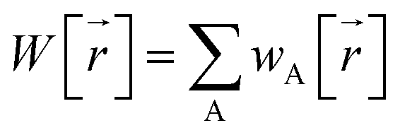 | (3) |
If this were true, then the Becke method should never assign a negative number of electrons to an atom in a material, and thus the Becke partial atomic charge should never exceed the atomic number. Since some of the Becke partial atomic charges for H, C, and N reported in Cho et al.'s dataset6 exceeded those elements' atomic numbers, there must be an underlying problem with how they were computed. Therefore, I had to remove all the Becke method data from this dataset when performing further statistical analysis.
The last three columns in Table 1 list the average, minimum, and maximum charge of each chemical element across the dataset of 25 charge assignment methods that does not include the Becke method. Except for H, the maximum atomic charge for each chemical element is now less than or equal to its atomic number. To better understand some of the atomic charges with large magnitudes, Table 2 lists details for each instance of a H atom having charge >1.00 and each instance of any other atom having a net charge larger in magnitude than 3.00. The ADCH and HLY methods gave some H atoms with charges >1.00; because these are not stockholder-type charge partitioning methods, they sometimes assign a negative number of electrons to an atom in a material. Several methods assigned atomic charges more negative than −3.00 to the C atom in CLi4 and/or CHLi5. The QTAIM method assigned atomic charges >3.00 to some of the P, S, and Si atoms in several molecules.
| Element | Atomic charges | Charge method | Systems |
|---|---|---|---|
| a One system with this stoichiometry had a ADCH charge of 1.30, while a different system with this same stoichiometry had a ADCH charge of 1.03. | |||
| H | 1.51, 1.30, 1.03 | ADCH | AlB2C2FH7MgNO, C18H22N4O14Pa |
| H | 1.07 | HLY | CHLi5 |
| C | −3.93, −3.78 | HLY | Li4C, CHLi5 |
| C | −4.02 | ISA | Li4C |
| C | −3.81 | MBIS | Li4C |
| C | −3.35 | NPA | Li4C |
| C | −3.38, −3.35 | QTAIM | CHLi5, Li4C |
| C | −3.52 | Ros-Schuit | CHLi5 |
| P | 3.14 to 3.81 | QTAIM | 41 different P atoms in various molecules |
| S | 3.11 to 3.89 | QTAIM | 16 different S atoms in various molecules |
| Si | 3.334, 3.327, 3.04 | QTAIM | SiF4, AlBF4H6OSSi2 |
Returning to the box plots in Fig. 1, the CM5, EEQ, Hirshfeld, and VDD methods gave the smallest ranges of atomic charges; atomic charges for these methods were between −1.5 and +1.5. The previously computed average charge transfer magnitudes for these molecular systems followed the order Hirshfeld < VDD < Mulliken < ACP < CM5 < ADCH < EEQ <⋯ < QTAIM.1 From these two observations, we conclude the Hirshfeld and VDD methods consistently give relatively small magnitudes of atomic charges. Behavior of the ISA method is interesting, because although its average charge transfer magnitude1 is moderate, sometimes it gives outliers with high magnitudes. For example, the atomic charge of C in Li4C was −4.02. If each Li atom only retained its core electrons the C atomic charge in this molecule would be −4. The ISA charge of −4.02 appears to indicate a slight loss of core electrons from the Li atoms, which seems physically dubious. For reasons that are not currently understood, for the Ros-Schuit method the Br atom box plot showed an extremely large range compared to the Br atom box plot for all of the other charge assignment methods.
For 16 of the charge assignment methods, the most negative C atom was in the Li4C molecule: ACP, Bickelhaupt, CHELPG, CM5, DDEC6, EEQ, Hirshfeld-I, HLY, IBO, ISA, MBIS, MBSMulliken, MK, NPA, RESP, and Stout-Politzer. For 19 of the charge assignment methods, the most positive Si atom was in the SiF4 molecule: APT, Bickelhaupt, CHELPG, DDEC6, Hirshfeld-I, HLY, i-ACP, IBO, ISA, MBIS, MBSBickelhaupt, MBSMulliken, MK, Mulliken, NPA, QTAIM, RESP, Ros-Schuit, and Stout-Politzer. For 14 of the charge assignment methods, the most positive Al atom was in the AlF3 molecule: Bickelhaupt, CHELPG, DDEC6, HLY, i-ACP, IBO, ISA, MBIS, MBSBickelhaupt, MBSMulliken, MK, NPA, RESP, and Ros-Schuit.
To better understand these results, Fig. 2 plots the Foster-Boys localized valence orbitals of Li4C, AlF3, and SiF4. In Li4C, these localized valence orbitals have a tetrahedral symmetry with most of the electron density located on the C atom; however, there is clearly some shared electron density in the bonding regions between the C and Li atoms. The AlF3 molecule is planar with most of the electron density of the valence orbitals located on the F atoms; however, there is clearly some shared electron density in the bonding regions between the Al and F atoms. The SiF4 molecule is tetrahedral with most of the electron density of the valence orbitals located on the F atoms; however, there is clearly some shared electron density in the bonding regions between the Si and F atoms. These results reflect the element electronegativity values. F is more electronegative than Al and Si.38–40 C is more electronegative than Li.38–40 These orbital plots show the DDEC6 computed atomic charges of −2.88 for C in Li4C, 1.84 for Al in AlF3, and 1.84 for Si in SF4 are plausible.
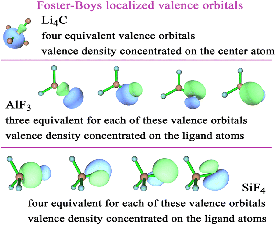 | ||
| Fig. 2 Foster-Boys localized orbitals for Li4C, AlF3, and SiF4 computed with the PBE0 exchange–correlation functional and def2tzvpp basis sets. | ||
3.2 Comparing standardized to unstandardized PCA over identical datasets
In this section, standardized PCA is compared to unstandardized PCA over identical datasets. Although such a comparison is not revolutionary science, it nevertheless is a significant scientific advance in two respects. The prior studies of Cho et al. for unstandardized PCA and Manz for standardized PCA included some bad datapoints and were performed over somewhat different subsets of the same parent dataset.1,6 Cho et al.'s study included a small number of missing and bad datapoints that were corrected or removed in Manz's study.1 Moreover, both of those studies included the Becke data that are shown in the previous section to be erroneous. This raises the question of how robust the conclusions of those studies are to the removal of the bad datapoints.As proved in ref. 1, for standardized PCA some performance measures are robust to corruption of any one of the independent descriptors. This robustness arises, because in standardized PCA each one of the independent descriptors contributes exactly 1.0 to the trace of the correlation matrix. For example, when performing standardized PCA over a set of 20 independent descriptors, each independent descriptor contributes exactly 5% to the trace of the correlation matrix: 1.0/20.0 = 5%. As a consequence, standardized PCA limits the potential impact that could be incurred by an error in one of the independent descriptors. This robustness is obviously a key advantage of using standardized PCA as opposed to using unstandardized PCA.
In unstandardized PCA, the contributions of different independent descriptors to the trace of the variance–covariance matrix can be different. Consequently, a large corruption of one of the independent descriptors can have an uncontrolled impact on the unstandardized PCA results. As shown in Section 3.1 above, the Becke charges in Cho et al.'s dataset were corrupted by a large amount. Because of this, it is not safe to assume that the unstandardized PCA results or conclusions that were reported by Cho et al.6 would automatically still hold once these bad datapoints are removed. Therefore, the conclusions of ref. 6 cannot automatically be assumed valid once it is discovered that some bad datapoints were included in their study.
In my view, the best way to resolve these issues is to reanalyze the dataset using both standardized PCA and unstandardized PCA with the bad datapoints removed. Such a reanalysis shows which of the previously proposed conclusions are valid and which are invalid (if any). It is absolutely essential to perform and publish such a reanalysis with the bad datapoints removed; otherwise, the unstandardized PCA results and conclusions that were reported by Cho et al.6 have to be set aside as inconclusive (i.e., as no longer conclusive), because their validity cannot be established without such a reanalysis.
In addition to the issue of bad datapoints discussed above, a second issue that needs to be addressed is the previously published unstandardized PCA included a slightly different subset of charge assignment methods than the previously published standardized PCA. Cho et al. reported that the MBSBickelhaupt and Hirshfeld-I atomic charges were most strongly correlated to the PC1 of unstandardized PCA including 16 charge assignment methods; the DDEC6 and MBIS methods also exhibited almost as high of correlations to PC1.6 Manz reported that the DDEC6 atomic charges consistently exhibited the highest correlations to PC1 for standardized PCA across 20 methods with a complete basis set limit and across all 26 charge assignment methods; the MBIS, ISA, and Hirshfeld-I methods also exhibited almost as high of correlations to PC1. When including all 26 methods, the MBSBickelhaupt method also exhibited almost as high correlation to PC1 in standardized PCA as DDEC6 and MBIS.1 The second question that must be addressed is whether differences in the conclusions of those two studies is due to standardized versus unstandardized PCA or whether it is due to the use of slightly different datasets (e.g., the inclusion of sligthly different subsets of charge assignment methods) for the analysis. The only way to definitively address this question is to perform unstandardized and standardized PCA on the same dataset and compare results.
Here, I performed standardized and unstandardized PCA on a dataset of 19 charge assignment methods having a complete basis set limit and across all 25 charge assignment methods. These datasets do not include the Becke method data. Table 3 summarizes the eigenvalues and the percentage of covariance (for unstandardized PCA) or correlation (for standardized PCA) accounted for by each principal component. In all cases, PC1 accounted for between 84.5% to 87.8% of the covariance or correlation while PC2 accounted for ≤7.1%. When using 19 charge methods with a complete basis set limit, PC2 in standardized PCA accounted for less than one variable's worth of correlation. On the other hand, when included all 25 charge methods, PC2 in standardized PCA accounted for 1.06 variable's worth of correlation; thus, PC2 may be considered significant in this case.
| Charge methods | PC1 | PC2 | PC3 | PC4 | % applies to | |
|---|---|---|---|---|---|---|
| Unstandardized | 19 | 1.835 (86.7%) | 0.151 (7.1%) | 0.060 (2.8%) | 0.020 (1.0%) | Covariance |
| Standardized | 19 | 16.683 (87.8%) | 0.811 (4.3%) | 0.554 (2.9%) | 0.307 (1.6%) | Correlation |
| Unstandardized | 25 | 2.502 (84.5%) | 0.201 (6.8%) | 0.096 (3.2%) | 0.070 (2.4%) | Covariance |
| Standardized | 25 | 21.678 (86.7%) | 1.059 (4.2%) | 0.616 (2.5%) | 0.445 (1.8%) | Correlation |
Coefficients for the first three principal components and correlation of each charge method to PC1 are listed in Table 4 (19 methods unstandardized PCA), Table 5 (19 methods standardized PCA), Table 6 (25 methods unstandardized PCA), and Table 7 (25 methods standardized PCA). Using the same notation as in ref. 1, the kth principal component's value for the ith datapoint (i.e., P(k)i) is the following normalized linear combination of the various independent descriptors:
| P(k)i = C(k,j)X(j)i | (4) |
 | (5) |
907 datapoints representing the different atoms in materials. In this work, the independent descriptors are the different methods for assigning atomic charges (e.g., DDEC6, Hirshfeld, QTAIM, VDD, etc.). The total number of independent descriptors (e.g., the number of different charge assignment methods) included in the PCA is V, and eqn (5) is the corresponding normalization condition for the kth principal component.1 If {X(j)} are unstandardized variables, the corresponding PCA is called unstandardized PCA. If {X(j)} are standardized variables, the corresponding PCA is called standardized PCA. As evident from the results presented in Tables 4–7, the values of the coefficients {C(k,j)} are generally different for standardized PCA compared to unstandardized PCA.
| Charge method | PC1 coefficient | PC2 coefficient | PC3 coefficient | Charge method | Correlation to PC1 |
|---|---|---|---|---|---|
| QTAIM | 0.414 | 0.715 | −0.151 | Hirshfeld-I | 0.983 |
| MBSMulliken | 0.294 | −0.286 | −0.483 | DDEC6 | 0.982 |
| MBIS | 0.275 | −0.128 | −0.083 | MBIS | 0.980 |
| Hirshfeld-I | 0.274 | −0.035 | −0.133 | ISA | 0.980 |
| APT | 0.258 | 0.389 | 0.117 | i-ACP | 0.965 |
| ISA | 0.254 | −0.057 | 0.185 | CHELPG | 0.953 |
| HLY | 0.234 | −0.237 | 0.350 | ACP | 0.949 |
| MK | 0.230 | −0.150 | 0.372 | RESP | 0.944 |
| CHELPG | 0.226 | −0.044 | 0.362 | MK | 0.941 |
| DDEC6 | 0.225 | −0.104 | −0.064 | IBO | 0.932 |
| RESP | 0.225 | −0.139 | 0.355 | MBSMulliken | 0.919 |
| IBO | 0.222 | −0.169 | −0.314 | HLY | 0.916 |
| i-ACP | 0.213 | 0.109 | 0.050 | CM5 | 0.912 |
| ACP | 0.155 | −0.075 | −0.065 | EEQ | 0.908 |
| EEQ | 0.154 | −0.118 | −0.128 | Hirshfeld | 0.901 |
| CM5 | 0.150 | −0.142 | −0.120 | VDD | 0.899 |
| ADCH | 0.142 | −0.209 | −0.096 | QTAIM | 0.890 |
| VDD | 0.088 | −0.007 | −0.038 | APT | 0.886 |
| Hirshfeld | 0.085 | −0.028 | −0.051 | ADCH | 0.842 |
| Charge method | PC1 coefficient | PC2 coefficient | PC3 coefficient | Correlation to PC1 |
|---|---|---|---|---|
| DDEC6 | 0.242 | 0.028 | 0.000 | 0.987 |
| MBIS | 0.240 | 0.028 | 0.027 | 0.982 |
| ISA | 0.240 | −0.090 | 0.172 | 0.978 |
| Hirshfeld-I | 0.239 | −0.067 | −0.044 | 0.975 |
| ACP | 0.236 | 0.087 | −0.095 | 0.965 |
| CHELPG | 0.233 | −0.126 | 0.331 | 0.953 |
| i-ACP | 0.233 | −0.247 | −0.059 | 0.953 |
| RESP | 0.233 | −0.010 | 0.388 | 0.951 |
| MK | 0.232 | −0.006 | 0.407 | 0.949 |
| IBO | 0.231 | 0.168 | −0.182 | 0.943 |
| CM5 | 0.231 | 0.253 | −0.139 | 0.942 |
| EEQ | 0.228 | 0.211 | −0.149 | 0.933 |
| MBSMulliken | 0.228 | 0.239 | −0.155 | 0.932 |
| HLY | 0.227 | 0.098 | 0.437 | 0.929 |
| Hirshfeld | 0.226 | 0.051 | −0.283 | 0.925 |
| VDD | 0.225 | −0.022 | −0.302 | 0.919 |
| ADCH | 0.216 | 0.381 | −0.070 | 0.883 |
| APT | 0.208 | −0.537 | −0.123 | 0.848 |
| QTAIM | 0.206 | −0.511 | −0.221 | 0.842 |
| Charge method | PC1 coefficient | PC2 coefficient | PC3 coefficient | Charge method | Correlation to PC1 |
|---|---|---|---|---|---|
| QTAIM | 0.344 | −0.635 | −0.396 | MBSBickelhaupt | 0.989 |
| NPA | 0.260 | 0.139 | −0.005 | DDEC6 | 0.985 |
| MBSMulliken | 0.259 | 0.219 | 0.006 | MBIS | 0.985 |
| MBSBickelhaupt | 0.239 | −0.002 | −0.068 | Hirshfeld-I | 0.982 |
| MBIS | 0.237 | 0.037 | 0.095 | ISA | 0.970 |
| Hirshfeld-I | 0.235 | −0.045 | 0.072 | Bickelhaupt | 0.965 |
| Stout-Politzer | 0.230 | 0.204 | −0.004 | NPA | 0.961 |
| ISA | 0.216 | −0.048 | 0.157 | ACP | 0.959 |
| APT | 0.215 | −0.370 | −0.147 | IBO | 0.951 |
| Bickelhaupt | 0.204 | 0.051 | −0.035 | i-ACP | 0.951 |
| Ros-Schuit | 0.200 | 0.500 | −0.647 | MBSMulliken | 0.947 |
| HLY | 0.200 | 0.066 | 0.353 | CHELPG | 0.935 |
| MK | 0.194 | 0.001 | 0.295 | RESP | 0.932 |
| DDEC6 | 0.194 | 0.022 | 0.098 | CM5 | 0.931 |
| IBO | 0.194 | 0.108 | 0.033 | MK | 0.930 |
| RESP | 0.190 | −0.002 | 0.277 | EEQ | 0.929 |
| CHELPG | 0.190 | −0.075 | 0.218 | Mulliken | 0.929 |
| i-ACP | 0.180 | −0.137 | −0.038 | Stout-Politzer | 0.925 |
| EEQ | 0.135 | 0.098 | −0.048 | HLY | 0.911 |
| ACP | 0.134 | 0.041 | −0.001 | Hirshfeld | 0.904 |
| CM5 | 0.131 | 0.105 | −0.004 | VDD | 0.899 |
| ADCH | 0.125 | 0.146 | 0.067 | QTAIM | 0.864 |
| Mulliken | 0.117 | 0.089 | 0.054 | ADCH | 0.863 |
| VDD | 0.075 | −0.008 | −0.012 | APT | 0.859 |
| Hirshfeld | 0.073 | 0.006 | 0.008 | Ros-Schuit | 0.694 |
| Charge method | PC1 coefficient | PC2 coefficient | PC3 coefficient | Correlation to PC1 |
|---|---|---|---|---|
| DDEC6 | 0.212 | −0.028 | 0.032 | 0.987 |
| MBIS | 0.211 | −0.019 | 0.035 | 0.983 |
| MBSBickelhaupt | 0.211 | −0.024 | −0.126 | 0.982 |
| Hirshfeld-I | 0.209 | −0.096 | −0.053 | 0.974 |
| ISA | 0.208 | −0.147 | 0.146 | 0.970 |
| ACP | 0.208 | 0.047 | −0.031 | 0.967 |
| Bickelhaupt | 0.207 | 0.051 | −0.134 | 0.966 |
| NPA | 0.206 | 0.123 | −0.112 | 0.959 |
| IBO | 0.205 | 0.126 | −0.089 | 0.955 |
| MBSMulliken | 0.204 | 0.201 | −0.076 | 0.949 |
| CM5 | 0.204 | 0.185 | −0.005 | 0.949 |
| Mulliken | 0.203 | 0.150 | 0.031 | 0.947 |
| i-ACP | 0.202 | −0.235 | −0.114 | 0.942 |
| EEQ | 0.202 | 0.176 | −0.052 | 0.942 |
| RESP | 0.202 | −0.126 | 0.375 | 0.940 |
| CHELPG | 0.201 | −0.211 | 0.288 | 0.938 |
| MK | 0.201 | −0.124 | 0.390 | 0.938 |
| Stout-Politzer | 0.199 | 0.207 | −0.078 | 0.928 |
| Hirshfeld | 0.198 | 0.003 | −0.114 | 0.923 |
| HLY | 0.198 | −0.045 | 0.447 | 0.922 |
| VDD | 0.196 | −0.046 | −0.158 | 0.915 |
| ADCH | 0.191 | 0.254 | 0.141 | 0.889 |
| APT | 0.179 | −0.435 | −0.284 | 0.835 |
| QTAIM | 0.178 | −0.407 | −0.375 | 0.830 |
| Ros-Schuit | 0.151 | 0.454 | −0.186 | 0.701 |
For unstandardized PCA with 19 and 25 methods, the QTAIM method (which has the largest average charge transfer magnitude) had the highest coefficient in PC1 but relatively low correlation to PC1. The QTAIM method also had the largest magnitude coefficient in PC2. For unstandardized PCA with 19 methods having a complete basis set limit, the Hirshfeld-I, DDEC6, MBIS, and ISA methods had the highest correlation to PC1. For unstandardized PCA including all 25 methods, MBSBickelhaupt, DDEC6, MBIS, and Hirshfeld-I had the highest correlation to PC1. These results are roughly consistent with those reported by Cho et al. using a slightly different data subset derived from the same parent dataset, except that there is some minor reordering among the highly ranked methods.6
For standardized PCA, the rank of methods according to correlation to PC1 is always identical to the rank according to coefficient in PC1.1 For standardized PCA with 19 methods having a complete basis set limit, the DDEC6, MBIS, ISA, and Hirshfeld-I methods had the highest correlation to PC1. For standardized PCA including all 25 methods, the DDEC6, MBIS, MBSBickelhaupt, and Hirshfeld-I methods had the highest correlation to PC1. These rankings are identical to those when the Becke method is included, as previously reported in ref. 1. Specifically, rankings of the 19 methods in standardized PCA reported here are identical to those for the 20 methods reported in ref. 1, except the Becke method gets the last (i.e., 20th ranking) when it is added to the dataset. With the exception of CM5 which is effectively tied with MBSMulliken, and i-ACP which is effectively tied with EEQ, the ranking of the 25 methods in standardized PCA reported here are identical to those for the 26 methods reported in ref. 1, except the Becke method gets the last (i.e., 26th ranking) when it is added to the dataset.
For a more complete understanding of rankings in standardized PCA, Table 8 (19 methods) and Table 9 (25 methods) show the method rankings according to three additional ranking criteria: (a) the sum of correlations between all of the individual charge assignment methods and a particular charge assignment method,
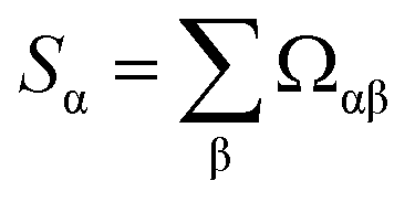 | (6) |
| Rank | Method | Sα | Ω[α,ϕ] | Method | Number (Ωαβ > 0.8) | Method | Number (Ωαβ > 0.9) |
|---|---|---|---|---|---|---|---|
| 1 | DDEC6 | 17.544 | 0.986 | DDEC6 | 19 | DDEC6 | 15 |
| 2 | MBIS | 17.455 | 0.981 | MBIS | 19 | MBIS | 14 |
| 3 | ISA | 17.401 | 0.978 | ISA | 19 | Hirshfeld-I | 11 |
| 4 | Hirshfeld-I | 17.345 | 0.975 | Hirshfeld-I | 19 | ISA | 10 |
| 5 | ACP | 17.159 | 0.965 | i-ACP | 18 | ACP | 9 |
| 6 | i-ACP | 16.960 | 0.953 | CHELPG | 18 | i-ACP | 9 |
| 7 | CHELPG | 16.946 | 0.953 | ACP | 17 | CHELPG | 9 |
| 8 | RESP | 16.909 | 0.951 | RESP | 17 | RESP | 8 |
| 9 | MK | 16.868 | 0.948 | MK | 17 | MK | 8 |
| 10 | IBO | 16.777 | 0.943 | IBO | 17 | MBSMulliken | 8 |
| 11 | CM5 | 16.742 | 0.941 | CM5 | 17 | CM5 | 7 |
| 12 | EEQ | 16.585 | 0.932 | EEQ | 17 | HLY | 7 |
| 13 | MBSMulliken | 16.570 | 0.932 | MBSMulliken | 17 | IBO | 6 |
| 14 | HLY | 16.508 | 0.928 | Hirshfeld | 17 | EEQ | 6 |
| 15 | Hirshfeld | 16.458 | 0.925 | VDD | 17 | Hirshfeld | 3 |
| 16 | VDD | 16.367 | 0.920 | HLY | 16 | APT | 3 |
| 17 | ADCH | 15.692 | 0.882 | ADCH | 15 | QTAIM | 3 |
| 18 | APT | 15.124 | 0.850 | APT | 9 | VDD | 2 |
| 19 | QTAIM | 15.018 | 0.844 | QTAIM | 8 | ADCH | 1 |
| Rank | Method | Sα | Ω[α,ϕ] | Method | Number (Ωαβ > 0.8) | Method | Number (Ωαβ > 0.9) |
|---|---|---|---|---|---|---|---|
| 1 | DDEC6 | 22.915 | 0.986 | DDEC6 | 24 | DDEC6 | 20 |
| 2 | MBIS | 22.828 | 0.983 | MBIS | 24 | MBIS | 19 |
| 3 | MBSBickelhaupt | 22.811 | 0.982 | MBSBickelhaupt | 24 | MBSBickelhaupt | 16 |
| 4 | Hirshfeld-I | 22.615 | 0.973 | Hirshfeld-I | 24 | Hirshfeld-I | 14 |
| 5 | ISA | 22.532 | 0.970 | ISA | 24 | ACP | 14 |
| 6 | ACP | 22.474 | 0.967 | Bickelhaupt | 24 | Bickelhaupt | 14 |
| 7 | Bickelhaupt | 22.443 | 0.966 | i-ACP | 23 | ISA | 13 |
| 8 | NPA | 22.267 | 0.958 | ACP | 22 | MBSMulliken | 13 |
| 9 | IBO | 22.177 | 0.955 | NPA | 22 | Mulliken | 13 |
| 10 | MBSMulliken | 22.045 | 0.949 | IBO | 22 | NPA | 12 |
| 11 | CM5 | 22.039 | 0.949 | MBSMulliken | 22 | IBO | 11 |
| 12 | Mulliken | 22.003 | 0.947 | CM5 | 22 | CM5 | 11 |
| 13 | EEQ | 21.887 | 0.942 | Mulliken | 22 | i-ACP | 10 |
| 14 | i-ACP | 21.887 | 0.942 | EEQ | 22 | CHELPG | 10 |
| 15 | RESP | 21.811 | 0.939 | RESP | 22 | Stout-Politzer | 10 |
| 16 | CHELPG | 21.775 | 0.937 | CHELPG | 22 | EEQ | 8 |
| 17 | MK | 21.763 | 0.937 | MK | 22 | RESP | 8 |
| 18 | Stout-Politzer | 21.550 | 0.928 | Hirshfeld | 22 | MK | 8 |
| 19 | Hirshfeld | 21.444 | 0.923 | HLY | 21 | HLY | 7 |
| 20 | HLY | 21.386 | 0.921 | VDD | 21 | Hirshfeld | 4 |
| 21 | VDD | 21.268 | 0.915 | Stout-Politzer | 20 | APT | 3 |
| 22 | ADCH | 20.657 | 0.889 | ADCH | 20 | QTAIM | 3 |
| 23 | APT | 19.411 | 0.836 | APT | 11 | VDD | 2 |
| 24 | QTAIM | 19.311 | 0.831 | QTAIM | 10 | ADCH | 1 |
| 25 | Ros-Schuit | 16.387 | 0.705 | Ros-Schuit | 1 | Ros-Schuit | 1 |
(b) the number of charge assignment methods having correlation Ωαβ > 0.8 to a particular charge assignment method, and (c) the number of charge assignment methods having correlation Ωαβ > 0.9 to a particular charge assignment method. As proved in ref. 1, ranking criterion (a) is equivalent to ranking the methods according to their correlation Ω[α,ϕ] to the average standardized variable ϕ. With some relatively minor differences, the rankings are approximately consistent between these three ranking criteria and the ranking according to correlation to PC1. The rankings in Table 8 (which does not include the Becke method) turned out to be identical to those reported in ref. 1 (which includes the Becke method), except the Becke method takes the last (i.e., 20th place) when added. The rankings in Table 9 (which does not include the Becke method) turned out to be identical to those reported in ref. 1 (which includes the Becke method), except the Becke method takes the last (i.e., 26th place) when added and there is a transposition of two adjacent methods (i.e., CM5 and MBSMulliken) in the ranking according to Sα.
Since there was a problem with the reported Becke atomic charges being incorrectly computed, no information is currently known about how the Becke atomic charges would perform if they would be computed correctly. The last ranking for the Becke method in ref. 1 may simply be a reflection of the fact that the reported Becke charges were computed incorrectly. Thus, this should not be taken as evidence that the Becke charge assignment method necessarily performs poorly if correctly implemented. To address the true performance of the Becke charge assignment method, an entirely new set of Becke charges would have to be computed across the molecular systems in this dataset. However, this is not feasible within the scope of present study, because Cho et al.'s dataset does not specifically give the XYZ coordinates of each atom along with the reported atomic charges. It is true the geometries were taken from the GMTKN55 collection, but matching the individual reported atomic charges to the individual geometries in the GMTKN55 collection would be tedious and not straightforward.
4. Conclusions
In prior literature, a detailed standardized PCA was performed on a slightly different dataset than a detailed unstandardized PCA, even though both datasets were derived from a common parent dataset.1,6 The slight differences in datasets made interpreting the differing conclusions of those two works difficult.To address this issue, herein I compared standardized to unstandardized PCA for the same dataset of partial atomic charges computed across ∼2000 molecules using various charge assignment methods. This analysis was performed both for 19 charge assignment methods having a complete basis set limit and for all 25 charge assignment methods, which do not include the Becke method.
Analysis of maximum and minimum charge values together with box plots for each chemical element for each charge assignment method revealed important information. Most importantly, the reported Becke charges were found to be incorrectly computed. The Becke method is generally believed to be a stockholder-type charge partitioning approach that assigns a non-negative number of electrons to each atom in a material; however, the Becke charges reported by Cho et al.6 showed several instances of assigning negative numbers of electrons to atoms. Consequently, the Becke charge data was not included in the PCA of the present study.
Many of the charge assignment methods exhibited large charge magnitudes for the Li4C, SiF4, and AlF3 molecules. Each of these molecules has two chemical elements with a large electronegativity difference. To understand this behavior better, localized valence orbitals for these three molecules were plotted in Fig. 2. These localized valence orbitals showed high bond polarities with electron density concentrated on the more electronegative atom(s) and in the bonding regions between atoms.
The main takeaways from this work are as follows. First, standardized PCA yielded more consistent rankings both across different ranking criteria and with respect to adding or removing some methods from the analysis. Second, the following five methods (listed here in alphabetical order) showed the greatest correlation to the first principal component in standardized and unstandardized PCA: DDEC6, Hirshfeld-I, ISA, MBIS, and MBSBickelhaupt (note: MBSBickelhaupt does not appear in the 19 methods dataset). For standardized PCA, the DDEC6 method ranked first followed closely by MBIS. For unstandardized PCA, Hirshfeld-I (19 methods) or MBSBickelhaupt (25 methods) ranked first followed by DDEC6 in second place (both 19 and 25 methods).
For a proper context, the above conclusions of this work must also be considered in light of the following known properties (established in the prior literature not in this work) of these five charge assignment methods. MBSBickelhaupt is not recommended, because its atomic charges are sensitive to rotation of the external coordinate system.1 ISA often gives erratic results for materials with buried atoms.1,41,42 For molecules, the average charge transfer magnitudes follow the trend MBSBickelhaupt ≈ MBIS ≈ Hirshfeld-I > ISA > DDEC6 ≈ electrostatic potential fitting charges.1 DDEC6 charges have been more thoroughly tested and shown to work across a wider range of material types including many dense solids.13,43
Conflicts of interest
There are no conflicts of interest to declare.Acknowledgements
National Science Foundation (NSF) CAREER Award DMR-1555376 provided financial support. The quantum chemistry calculations of Li4C, AlF3, and CF4 were performed on the Expanse supercomputer at the San Diego Supercomputing Center using project allocation TG-CTS100027 on the Extreme Science and Engineering Discovery Environment (XSEDE). XSEDE was funded by NSF grant ACI-1548562.44References
- T. A. Manz, Seven confluence principles: a case study of standardized statistical analysis for 26 methods that assign net atomic charges in molecules, RSC Adv., 2020, 10, 44121–44148 RSC.
- F. Heidar-Zadeh, P. W. Ayers, T. Verstraelen, I. Vinogradov, E. Vohringer-Martinez and P. Bultinck, Information-theoretic approaches to atoms-in-molecules: Hirshfeld family of partitioning schemes, J. Phys. Chem. A, 2018, 122, 4219–4245 CrossRef CAS PubMed.
- J. Cioslowski, A new population analysis based on atomic polar tensors, J. Am. Chem. Soc., 1989, 111, 8333–8336 CrossRef CAS.
- T. Chen and T. A. Manz, A collection of forcefield precursors for metal-organic frameworks, RSC Adv., 2019, 9, 36492–36507 RSC.
- I. T. Jolliffe and J. Cadima, Principal component analysis: a review and recent developments, Philos. Trans. R. Soc., A, 2016, 374, 20150202 CrossRef PubMed.
- M. Cho, N. Sylvetsky, S. Eshafi, G. Santra, I. Efremenko and J. M. L. Martin, The atomic partial charges arboretum: Trying to see the forest for the trees, ChemPhysChem, 2020, 21, 688–696 CrossRef CAS PubMed.
- L. Goerigk, A. Hansen, C. Bauer, S. Ehrlich, A. Najibi and S. Grimme, A look at the density functional theory zoo with the advanced GMTKN55 database for general main group thermochemistry, kinetics and noncovalent interactions, Phys. Chem. Chem. Phys., 2017, 19, 32184–32215 RSC.
- A. A. Voityuk, A. J. Stasyuk and S. F. Vyboishchikov, A simple model for calculating atomic charges in molecules, Phys. Chem. Chem. Phys., 2018, 20, 23328–23337 RSC.
- T. Lu and F. W. Chen, Atomic dipole moment corrected Hirshfeld population method, J. Theor. Comput. Chem., 2012, 11, 163–183 CrossRef CAS.
- A. D. Becke, A multicenter numerical-integration scheme for polyatomic molecules, J. Chem. Phys., 1988, 88, 2547–2553 CrossRef CAS.
- C. M. Breneman and K. B. Wiberg, Determining atom-centered monopoles from molecular electrostatic potentials - the need for high sampling density in formamide conformational analysis, J. Comput. Chem., 1990, 11, 361–373 CrossRef CAS.
- A. V. Marenich, S. V. Jerome, C. J. Cramer and D. G. Truhlar, Charge Model 5: An extension of Hirshfeld population analysis for the accurate description of molecular interactions in gaseous and condensed phases, J. Chem. Theory Comput., 2012, 8, 527–541 CrossRef CAS PubMed.
- T. A. Manz and N. Gabaldon Limas, Introducing DDEC6 atomic population analysis: part 1. Charge partitioning theory and methodology, RSC Adv., 2016, 6, 47771–47801 RSC.
- S. A. Ghasemi, A. Hofstetter, S. Saha and S. Goedecker, Interatomic potentials for ionic systems with density functional accuracy based on charge densities obtained by a neural network, Phys. Rev. B, 2015, 92, 045131 CrossRef.
- F. L. Hirshfeld, Bonded-atom fragments for describing molecular charge densities, Theor. Chim. Acta, 1977, 44, 129–138 CrossRef CAS.
- G. Knizia, An unbiased bridge between quantum theory and chemical concepts, J. Chem. Theory Comput., 2013, 9, 4834–4843 CrossRef CAS PubMed.
- H. Hu, Z. Y. Lu and W. T. Yang, Fitting molecular electrostatic potentials from quantum mechanical calculations, J. Chem. Theory Comput., 2007, 3, 1004–1013 CrossRef CAS PubMed.
- S. F. Vyboishchikov and A. A. Voityuk, Iterative atomic charge partitioning of valence electron density, J. Comput. Chem., 2019, 40, 875–884 CrossRef CAS PubMed.
- P. Bultinck, C. Van Alsenoy, P. W. Ayers and R. Carbo-Dorca, Critical analysis and extension of the Hirshfeld atoms in molecules, J. Chem. Phys., 2007, 126, 144111 CrossRef PubMed.
- T. C. Lillestolen and R. J. Wheatley, Redefining the atom: Atomic charge densities produced by an iterative stockholder approach, Chem. Commun., 2008, 5909–5911 RSC.
- T. Verstraelen, S. Vandenbrande, F. Heidar-Zadeh, L. Vanduyfhuys, V. Van Speybroeck, M. Waroquier and P. W. Ayers, Minimal basis iterative stockholder: atoms in molecules for force-field development, J. Chem. Theory Comput., 2016, 12, 3894–3912 CrossRef CAS PubMed.
- J. A. Montgomery, M. J. Frisch, J. W. Ochterski and G. A. Petersson, A complete basis set model chemistry. VII. Use of the minimum population localization method, J. Chem. Phys., 2000, 112, 6532–6542 CrossRef CAS.
- B. H. Besler, K. M. Merz and P. A. Kollman, Atomic charges derived from semiempirical methods, J. Comput. Chem., 1990, 11, 431–439 CrossRef CAS.
- R. F. W. Bader and P. M. Beddall, Virial field relationship for molecular charge distributions and spatial partitioning of molecular properties, J. Chem. Phys., 1972, 56, 3320–3329 CrossRef CAS.
- C. I. Bayly, P. Cieplak, W. D. Cornell and P. A. Kollman, A well-behaved electrostatic potential based method using charge restraints for deriving atomic charges - the RESP model, J. Phys. Chem., 1993, 97, 10269–10280 CrossRef CAS.
- C. F. Guerra, J. W. Handgraaf, E. J. Baerends and F. M. Bickelhaupt, Voronoi deformation density (VDD) charges: Assessment of the Mulliken, Bader, Hirshfeld, Weinhold, and VDD methods for charge analysis, J. Comput. Chem., 2004, 25, 189–210 CrossRef CAS PubMed.
- F. M. Bickelhaupt, N. J. R. V. Hommes, C. F. Guerra and E. J. Baerends, The carbon-lithium electron pair bond in (CH3Li)n (n=1, 2, 4), Organometallics, 1996, 15, 2923–2931 CrossRef CAS.
- R. S. Mulliken, Electronic population analysis on LCAO-MO molecular wave functions, J. Chem. Phys., 1955, 23, 1833–1840 CrossRef CAS.
- A. E. Reed, R. B. Weinstock and F. Weinhold, Natural population analysis, J. Chem. Phys., 1985, 83, 735–746 CrossRef CAS.
- P. Ros and G. C. A. Schuit, Molecular orbital calculations on copper chloride complexes, Theor. Chim. Acta, 1966, 4, 1–12 CrossRef CAS.
- E. W. Stout and P. Politzer, An investigation of definitions of charge on an atom in a molecule, Theor. Chim. Acta, 1968, 12, 379–386 CrossRef CAS.
- J. P. Perdew, K. Burke and M. Ernzerhof, Generalized gradient approximation made simple, Phys. Rev. Lett., 1996, 77, 3865–3868 CrossRef CAS PubMed.
- C. Adamo and V. Barone, Toward reliable density functional methods without adjustable parameters: The PBE0 model, J. Chem. Phys., 1999, 110, 6158–6170 CrossRef CAS.
- F. Weigend and R. Ahlrichs, Balanced basis sets of split valence, triple zeta valence and quadruple zeta valence quality for H to Rn: Design and assessment of accuracy, Phys. Chem. Chem. Phys., 2005, 7, 3297–3305 RSC.
- M. J. Frisch, G. W. Trucks, H. B. Schlegel, G. E. Scuseria, M. A. Robb, J. R. Cheeseman, G. Scalmani, V. Barone, G. A. Petersson, H. Nakatsuji, X. Li, M. Caricato, A. V. Marenich, J. Bloino, B. G. Janesko, R. Gomperts, B. Mennucci, H. P. Hratchian, J. V. Ortiz, A. F. Izmaylov, J. L. Sonnenberg, D. Williams-Young, F. Ding, F. Lipparini, F. Egidi, J. Goings, B. Peng, A. Petrone, T. Henderson, D. Ranasinghe, V. G. Zakrzewski, J. Gao, N. Rega, G. Zheng, W. Liang, M. Hada, M. Ehara, K. Toyota, R. Fukuda, J. Hasegawa, M. Ishida, T. Nakajima, Y. Honda, O. Kitao, H. Nakai, T. Vreven, K. Throssell, J. A. Montgomery Jr, J. E. Peralta, F. Ogliaro, M. J. Bearpark, J. J. Heyd, E. N. Brothers, K. N. Kudin, V. N. Staroverov, T. A. Keith, R. Kobayashi, J. Normand, K. Raghavachari, A. P. Rendell, J. C. Burant, S. S. Iyengar, J. Tomasi, M. Cossi, J. M. Millam, M. Klene, C. Adamo, R. Cammi, J. W. Ochterski, R. L. Martin, K. Morokuma, O. Farkas, J. B. Foresman and D. J. Fox, Gaussian 16, Revision B.01, Gaussian, Inc., Wallingford CT, 2016 Search PubMed.
- J. M. Foster and S. F. Boys, Canonical configuration interaction procedure, Rev. Mod. Phys., 1960, 32, 300–302 CrossRef CAS.
- T. Lu and F. W. Chen, Multiwfn: A multifunctional wavefunction analyzer, J. Comput. Chem., 2012, 33, 580–592 CrossRef CAS PubMed.
- C. Tantardini and A. R. Oganov, Thermochemical electronegativities of the elements, Nat. Commun., 2021, 12, 2087 CrossRef CAS PubMed.
- Electronegativity, in CRC Handbook of Chemistry and Physics, ed. W. M. Haynes, CRC Press, Boca Raton, Florida, 97th edn, 2016, p. 9.103 Search PubMed.
- L. Pauling, The nature of the chemical bond: IV. The energy of single bonds and the relative electronegativity of atoms, J. Am. Chem. Soc., 1932, 54, 3570–3582 CrossRef CAS.
- T. A. Manz and D. S. Sholl, Chemically meaningful atomic charges that reproduce the electrostatic potential in periodic and nonperiodic materials, J. Chem. Theory Comput., 2010, 6, 2455–2468 CrossRef CAS PubMed.
- P. Bultinck, D. L. Cooper and D. Van Neck, Comparison of the Hirshfeld-I and iterated stockholder atoms in molecules schemes, Phys. Chem. Chem. Phys., 2009, 11, 3424–3429 RSC.
- N. Gabaldon Limas and T. A. Manz, Introducing DDEC6 atomic population analysis: part 2. Computed results for a wide range of periodic and nonperiodic materials, RSC Adv., 2016, 6, 45727–45747 RSC.
- J. Towns, T. Cockerill, M. Dahan, I. Foster, K. Gaither, A. Grimshaw, V. Hazlewood, S. Lathrop, D. Lifka, G. D. Peterson, R. Roskies, J. R. Scott and N. Wilkins-Diehr, XSEDE: accelerating scientific discovery, Comput. Sci. Eng., 2014, 16, 62–74 Search PubMed.
| This journal is © The Royal Society of Chemistry 2022 |