Determination of ethanol content during simultaneous saccharification and fermentation (SSF) of cassava based on a colorimetric sensor technique

Abstract

Ethanol content is an important indicator reflecting the yield of simultaneous saccharification and fermentation (SSF) of cassava. This study proposes an innovative method based on a colorimetric sensor technique to determine the ethanol content during the SSF of cassava. First, 14 kinds of porphyrin material and one kind of pH indicator were used to form a colorimetric sensor array for collecting odor data during the SSF of cassava. Then, the ant colony algorithm (ACO) and the simulated annealing algorithm (SA) were used to optimize and reconstruct the input color feature components of the support vector regression (SVR) model. The differential evolution algorithm (DE) was used to optimize the penalty factor (c) and the kernel function (g) of the SVR model. The results obtained showed that the combined prediction model of SA-DE-SVR had the highest accuracy, and the coefficient of determination (R_P²) in the prediction set was 0.9549, and the root mean square error of prediction (RMSEP) was 0.1562. The overall results reveal that the use of a colorimetric sensor technique combined with different intelligent optimization algorithms to establish a model can quantitatively determine the ethanol content in the SSF of cassava, and has broad development prospects.

---

1. Introduction

With the rapid development of China's economy, the demand for energy usage has increased dramatically, and traditional non-renewable energy sources have become increasingly unable to meet the country's sustainable development goals.¹ People are constantly looking for a renewable energy source to solve the current urgent need. As an emerging green and clean resource, fuel ethanol is not only convenient to use, environmentally friendly, but also has strong renewability, and is one of the important energies used in human life at present.² However, with the vigorous development of fuel ethanol, it is bound to put a certain burden on the national treasury's grain reserves.³ Therefore, with the limited supply of food, vigorously developing fuel ethanol production technology can not only avoid food waste, but also make ethanol production more efficient and achieve a perfect combination of production quality and technology.

Simultaneous saccharification and fermentation (SSF) usually refers to simultaneous cellulase hydrolysis and ethanol production fermentation in the same reactor.⁴ This production method not only avoids the infection of microbial strains caused by repeated replacement of the reaction device during the fermentation process, but also because the sugars produced during the hydrolysis process can be quickly converted into ethanol, which greatly improves the fermentation rate of ethanol.⁵ However, the SSF technology still has some shortcomings: the optimum temperature of hydrolysis is not consistent with the optimum temperature of fermentation, which is one of the reasons that affect the decline in ethanol production; secondly, enzymatic hydrolysis cannot stably maintain a moderate concentration of reducing sugars.⁴ This is also one of the reasons for the decline in ethanol production. Therefore, the establishment of a non-destructive detection technology for measuring the ethanol content in the SSF of cassava is of great significance for controlling the stability of the key parameters of the entire SSF.

Colorimetric sensor technique is a new development and application of electronic nose technique, which has been rising rapidly in recent years.⁶ It is more sensitive and stable than traditional electronic nose technique which relies too much on van der Waals forces.⁷ This makes this technology very suitable for the analysis of microbial parameters and population changes in the process of ethanol fermentation. However, the preparation of the colorimetric sensor array is the key to the successful application of this technique. Compared with the traditional olfactory sensor technique, the substrate and the color developer used in the colorimetric sensor are mostly hydrophobic materials, which makes the influence of the external environment humidity on it minimal. Among them, the substrate often chooses C2 inverted silica gel plate.⁸ The C2 inverted silica gel plate has a white bottom surface as a background, which is convenient for image processing. In addition, the small pore size on the surface is very conducive to the absorption of volatile gases. The color reagents are mostly sensitive and easy to absorb odor chemical reagents,⁹ which can cause color changes when reacting with volatile gases. According to the difference between the color changes before and after the reflection, the corresponding data difference is obtained for quantitative analysis.¹⁰ It is worth noting that most of these volatile odor concentrations have reached the ppb level, and these color developers can still react with them to produce changes, which highly reflects the characteristics of high sensitivity.¹¹ At present, colorimetric sensor technique has been widely used in food science,¹² medical science,¹³ environmental science¹⁴ etc., but there are still few articles on the parameter detection of the SSF of cassava. Therefore, the application of colorimetric sensor technique to the quantitative detection of ethanol content in the SSF of cassava will have broad development prospects.

But colorimetric sensor technique is not a very mature technology, and there are still places to be broken through in many aspects.¹⁵ First of all, in the selection and production of color-sensitive materials, porphyrin materials with stronger specificity and higher sensitivity can be screened out according to the composition of volatiles. Secondly, in terms of experimental data processing, in order to improve the overall input data quality, the swarm intelligence optimization algorithm can be used to reconstruct the input subsequence and optimize the input feature data. In the process of model construction, we can also use the intelligent algorithm to optimize the model parameters, and further improve the accuracy of the model.

This research introduces the method of combining colorimetric sensors and intelligent algorithms, and aims to provide a method that uses fast and non-destructive sensor detection technology to replace traditional detection methods, which greatly improves the sensitivity and accuracy of detection. Compared with the colorimetric sensor technology that has been widely used in food quality analysis in recent years, there are not many research results in the application of fermentation industry. Therefore, this research explored the development of a colorimetric sensor system, and then combined with the intelligent algorithm for quantitative analysis of ethanol fermentation content, thus verifying the feasibility of this technology, and hope that this technology can go out of the laboratory, applied to larger fields such as industry and agriculture.

The specific work of this study are as follows: (1) develop a colorimetric sensor array; (2) realize sample preparation and data collection in the SSF of cassava; (3) use a combination of multiple swarm intelligence algorithms to complete the establishment of the SVR quantitative model; (4) independent testing samples to verify the model.

2. Materials and methods

2.1 Fermentation sample preparation

First, wash and peel the purchased cassava and put it into an electric heating blast drying box at 80 °C for drying until the weight remains unchanged. Then use the laboratory's FW high-speed pulverizer to crush the cassava to make the particle size between 1–2 mm. Take out 180 g of particles and put them into three 250 mL volumetric flasks with labels A, B, and C on average, slowly pour 150 mL distilled water, and add 15 μg of high temperature resistant α-amylase. Put the prepared volumetric flask into a constant temperature water bath at 80 °C to liquefy for 90 minutes, then take it out and put it in a sterilizer for autoclaving for 40 minutes. Then, add 7 mL of yeast at the end of the logarithmic phase and 150 μg of glucoamylase (100, 000 μg) into 3 labeled volumetric flasks, seal, wrap and shake, and placed into a constant temperature oscillating chamber with a temperature of 30 °C and a speed of 200 rpm to continue the cassava SSF.

In this experiment, the time for a batch of cassava simultaneous saccharification and fermentation was 72 hours, during which sampling was conducted every 4 hours from the start of cassava fermentation, and a total of 19 times were sampled during the whole fermentation stage, respectively at 0 h, 4 h, 8 h, …, 72 h. In order to avoid continuous sampling resulting in the reduction of fermentation samples in the bottle and affecting subsequent fermentation, this experiment divided 19 sampling points into 3 segments. The first 7 time points (0 h, 4 h, …, 24 h) were carried out in volumetric flask A, and the middle 6 sampling time points (28 h, 32 h, …, 48 h) were carried out in volumetric flask B, and the remaining 6 sampling time points (52 h, 56 h, …, 72 h) were carried out in volumetric flask C. Using the same materials and methods for 8 batches of experiments, a total of 152 fermentation samples could be collected.

2.2 Ethanol content determination

The actual content of ethanol in the sample was determined by using potassium dichromate oxidation colorimetry. The specific steps were as follows: (1) draw a standard ethanol content curve: take 2 g of anhydrous ethanol into a 100 mL volumetric flask, add distilled water to make the volume to 100 mL and shake it up to get a 20 mg mL⁻¹ ethanol solution; then take 8 test tubes with a capacity of 30 mL, add 0, 0.1, 0.2, 0.4, 0.6, 0.8, 1.0 and 1.2 mL of the above-mentioned 20 mg mL⁻¹ ethanol solution into each test tube, add an appropriate amount of distilled water to fix the volume to 2 mL. Then, add 5 mL of 2% potassium dichromate solution and shake well, heat it in a boiling water bath for 10 minutes and take it out to cool, then add distilled water in each test tube to fix the volume to 25 mL and shake it evenly. Finally, set the wavelength of the ultraviolet spectrophotometer to 600 nm, take 2.5 mL of the solution into the cuvette to measure the OD value respectively, and make a blank zero adjustment. Keep the OD value between 0.1 and 0.7. If it exceeds this value, dilute it by a certain multiple and measure again. Using the ethanol content as the abscissa and the OD value as the ordinate, the linear correlation line between the ethanol content and the OD value can be obtained. The linear equation is: y = 0.0506x + 0.0021. (2) Put 1 g of the fermentation sample in a conical flask containing 50 mL of distilled water. After completion, put the Erlenmeyer flask in a constant temperature water bath at 55 °C for 20 minutes and then take it out to cool. Next, remove 8 mL from the cooled solution and put it in a centrifuge tube. At the same time, set the centrifuge speed to 12 000 rpm, put the centrifuge tube in the centrifuge for 10 minutes, and then remove 1 mL of the supernatant from the centrifuge. Put the liquid into a clean test tube, pour distilled water to make the volume up to 2 mL, add 5 mL potassium dichromate solution, heat it in a boiling water bath for 12 minutes, take it out, cool it down with flowing cold water, and then pour distilled water to make it final volume to 25 mL. After shaking well, take out 2.5 mL and pour it into a cuvette. Detect its OD value in a spectrophotometer with a wavelength of 600 nm (zero adjustment),¹⁶ and use the measured OD value combined with the ethanol standard curve to obtain the ethanol in the fermentation sample.

Fig. 1 shows the dynamic curve of ethanol content in the synchronous saccharification fermentation of ethanol. As can be seen from the figure, 0–8 h was the early stage of ethanol fermentation. At this time, ethanol production was slowly rising, and the overall trend was not obvious; during the main fermentation period of 8–48 h, ethanol showed a sharp rise, which was due to the rapid consumption of cassava sugar during the main fermentation period, and then converted into ethanol. 48–72 h was the late fermentation period. It can be seen that the growth of ethanol content was slow until it tended to be stable. This was because the sugar in cassava has been consumed and the whole fermentation process was over.

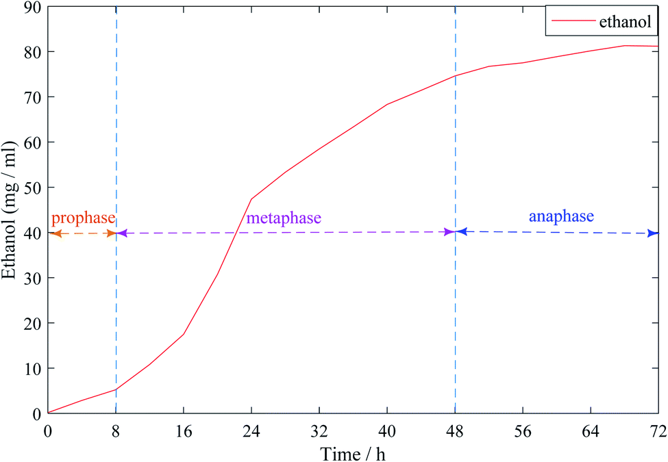Fig. 1 Dynamic curve of ethanol content in the process of ethanol simultaneous saccharification and fermentation.

2.3 Preparation of colorimetric sensor array

The preparation of the colorimetric sensor array is the key of this technique and has a crucial importance to carry on the top and bottom. Therefore, it must have two conditions: (1) each chemical reagent can produce a strong action reaction with the reactant odor; (2) each active center must have a strong coupling chromophore. According to the research of the GC-MS applied in cassava SSF process, it was determined that the major volatile odor components were acetic acid, propionic acid and butyric acid respectively.⁶ Therefore, by analyzing the results of the preliminary pre-experiments, 14 porphyrin compounds and one hydrophobic pH indicator were finally selected and used to form a 5 × 3 colorimetric sensor array. The selected gas-sensitive materials are listed in Table 1. For the preparation of colorimetric sensor array, the specific fabrication process was as follows: first, 6 mg of each of the 14 porphyrins were weighed and 3 mL of methylene chloride was added to dissolve it, and then 6 mg of the pH indicator was weighed and 3 mL of anhydrous ethanol was added to dissolve it, and the volume was adjusted to obtain 15 bottles of 2 mg L⁻¹ solution. The solution was ultrasonically shaken for half an hour to fully dissolve the solute. Next, the solution was stained on C2 reversed-phase silica gel plates (Merck, USA) one by one with a 0.3 mm diameter microcapillary, making sure that the size of each color-sensitive spot was the same as possible. Finally, the completed sensor arrays were dried in a fume hood and stored in a sealed dark environment for further use.

Table 1 Names of color-sensitive materials used to prepare colorimetric sensor

Number	Name
1	5,10,15,20-Tetraphenyl-21H,23H-porphine
2	5,10,15,20-Tetraphenyl-21H,23H-porphine manganese(III) chloride
3	5,10,15,20-Tetrakis(4-methoxyphenyl)-21H,23H-porphine iron(III) chloride
4	5,10,15,20-Tetraphenyl-21H,23H-porphine iron(III) chloride
5	5,10,15,20-Tetraphenyl-21H,23H-porphine zinc
6	2,3,7,8,12,13,17,18-Octaethyl-21H,23H-porphine nickel(II)
7	meso-Tetra(4-carboxyphenyl)porphine tetramethyl ester
8	meso-Tetraphenyl porphyrin (chlorine free)
9	2,3,7,8,12,13,17,18-Octaethyl-21H,23H-porphine cobalt(II)
10	2,3,7,8,12,13,17,18-Octaethyl-21H,23H-porphine manganese(III) chloride
11	2,3,7,8,12,13,17,18-Octaethyl-21H,23H-porphine
12	5,10,15,20-Tetraphenyl-21H,23H-porphine vanadium(IV) oxide
13	2,3,7,8,12,13,17,18-Octaethyl-21H,23H-porphine ruthenium(II) carbonyl
14	5,10,15,20-Tetrakis(4-methoxyphenyl)-21H,23H-porphine
15	Bromothymol blue

---

2.4 Data acquisition and pre-treatment

This experiment used the prepared colorimetric sensor array to collect data of the collected samples in the SSF of cassava, and the procedure was as follows: firstly, set the initial image resolution of the HP tablet scanner used for image capture to 300 dpi, and the primitive R, G, and B data images were obtained by scanning the colorimetric sensor array after the setup was completed. Then, 5 g of ferment sample was weighed into a 90 mm Petri dish, and the colorimetric sensor array before the reaction was fixed on the cling film using double-sided tape, and the Petri dish was sealed face down, after which it was placed at room temperature of 25 °C for 6 min and then removed, in particular, the time taken to reflect 6 min here was that we put the same concentration of ethanol for different times in the early stage, and used colorimetric sensor technology to conduct a pre-experiment to optimize the reaction time. The pre-experimental operation was consistent with the above content, and finally chose 6 min as the best response time. In this 6 min time, the porphyrin gas-sensing array could quickly respond to the odor information of ethanol, collected data that best reflects the odor information, and highly reflected the sensitivity of the sensor. Then, the sensor array was scanned again to get the image after the reaction. Finally, the images before and after the reaction were transferred to the computer image processing software, and the color difference values of the corresponding color-sensitive points were obtained after the steps of filtering and noise reduction, threshold segmentation of the image background plate, morphological processing, and central value extraction. Each color-sensitive point contains three color variables: ΔR, ΔG, and ΔB (ΔR = |R_n − R_m|, ΔG = |G_n − G_m|, ΔB = |B_n − B_m|). Since each sensor array has 15 color sensitive points, a total of 45 characteristic color components (15 points × 3 color components) can be obtained. In a batch of 19 sampling time points, the same operations were performed, with the difference that each time a clean Petri dish and a new sensor array reversed-phase silica gel plates were replaced to prevent contamination by bacteria and unwanted factors caused by the odor of residual samples from the previous batch, ensuring that the data we collected each time were accurate in real time. Such parallel experiments were conducted for a total of 8 batches. The data acquisition and pre-processing process of the colorimetric sensor system is shown in Fig. 2.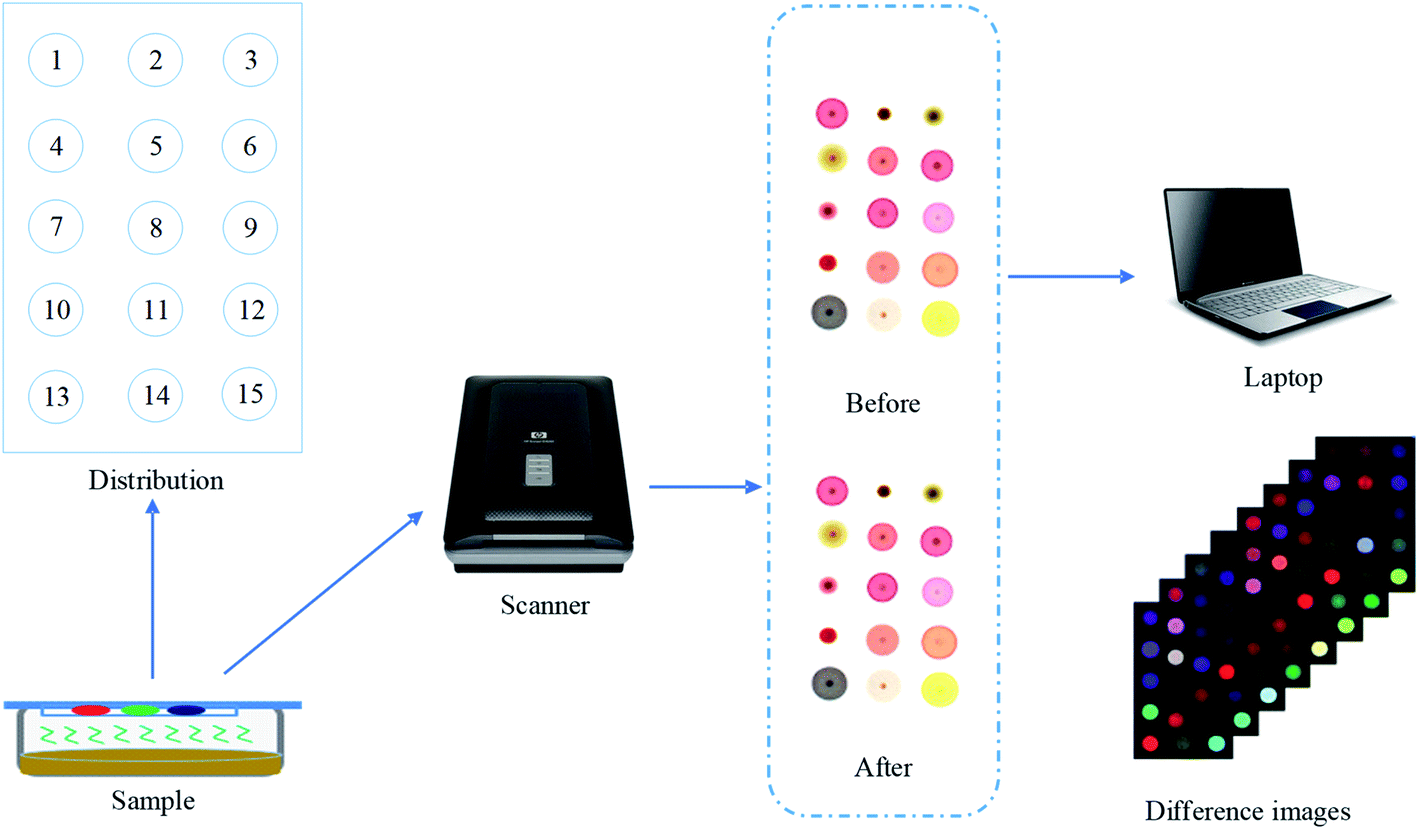

Fig. 2 Data acquisition and pre-processing of the colorimetric sensor system.

2.5 Data analysis method

2.5.1 Back-propagation neural network. Back-propagation neural network (BPNN) is one of the classical neural networks, and its full name is a neural network based on error back propagation algorithm.¹⁷ It is generally composed of three or more layers of neurons, respectively: input layer, hidden layer and output layer.¹⁸ When the signal is propagated from the input layer to the output layer through the implicit layer, the signal is propagated in the positive direction. When the output signal is the same as the desired signal, the algorithm is terminated; otherwise, the backward propagation of the error is continued, during which the error between the output value and the true value is equally distributed among the intermediate units, each of which uses the error signal as the basis for modifying the weights of each layer. The whole process is continuously propagated forward and backward, and the layer weights are continuously modified until the output error meets the initial expectation.¹⁹

In this study, the combination of BPNN model and intelligent optimization algorithm was used to complete the optimal reconstruction of the color component of the input features. Before running the Bp neural network, set the number of neurons in the hidden layer as 10, set the initial weights as 0.3, set the learning rate and momentum factor as 0.1, set the minimum allowable training error as 0.001, finally, set the maximum training times as 1000.

2.5.2 Support vector regression. Support vector regression (SVR) is a branch of support vector machine (SVM), which is widely used in solving nonlinear problems.²⁰ The core idea of the SVR model is to use the kernel function to transform and map a nonlinear problem into a high-dimensional space.²¹ In the high-dimensional space, the problem becomes a linear problem by constructing a linear decision function. For the linear function, it constructs an interval band on both sides of it, and if the training samples fall into the interval band, no loss is accounted for. If it falls outside the interval band, the loss function is included. Finally, the model is optimized by minimizing the interval and the total loss function, and there are several types of kernel functions for SVR: linear kernel, polynomial kernel, Gaussian kernel, radial basis kernel, and Sigmoid kernel, which we can choose according to the specific problem. Among them, linear kernel is suitable for samples with little data, Gaussian kernel is suitable for samples with high local requirement, while radial basis and Sigmoid are mostly suitable for neural networks and deep learning that require memory.²²

In this study, due to the small sample data, the radial basis kernel function was chosen to accomplish the classification prediction of this nonlinear sample. The parameters c, g of the SVR model were optimized using the DE algorithm, and then combined with the best input feature variables to build the best combined prediction regression model. Among them, the SVR model prediction centralized decision coefficient R_p² and the root mean square error of prediction RMSEP were used to make an evaluation basis for the model performance.

2.5.3 Ant colony algorithm. Ant colony algorithm (ACO) is a heuristic algorithm to find the optimal path, which is mainly divided into two parts: path construction, and pheromone update.²³ In nature, although ants are blind, they will automatically bypass obstacles to find another path when they encounter them. This phenomenon arises because they will release pheromones along the way, and the shorter the path, the more pheromones there are instead. Compared with a long path, ants usually choose a short path, while the pheromones will slowly disappear for long path lots. Eventually, all ants will find an optimal path, which forms a positive feedback mechanism. The ant colony algorithm can be well applied to the screening of image feature color components because of its strong global search ability and high robustness.²⁴

In this study, the ant colony algorithm combined with the BPNN model was used to optimize the input feature color components. Before running the program, set the initial value of the ant colony population size as 20, adjust the pheromone evaporation rate to 0.05, and set the maximum number of iterations as 100.

2.5.4 Simulated annealing algorithm. The simulated annealing algorithm (SA) is a stochastic shrinkage method extended according to the local search method.²⁵ The idea comes from a process in which a solid is first warmed up and melted and then annealed and solidified. It is now widely used in neural network science, image processing and other fields. The algorithm is an optimal solution algorithm based on the Monte Carlo idea, which first uses the Metropolis sampling criterion to select the local optimal solution, followed by introducing random factors in the search process to jump out of the local optimal solution, and then after a large number of solution changes, iterative changes, and control parameters, the global optimal solution is obtained. The algorithm not only has high sensitivity, but also strong ability to combine with other algorithms, and has good global optimization performance.

In this study, the simulated annealing algorithm combined with the BPNN model was used to find the best combination of sensor color feature components. Before running the SA algorithm, the initial temperature was set as 10, the annealing rate was 0.99, the maximum number of iterations was 100, and finally, the maximum number of sub-iterations was set as 20.

2.5.5 Differential evolution algorithm. The differential evolution (DE) algorithm is an algorithm that evolves by simulating the law of superiority and inferiority of organisms in nature.²⁶ The DE algorithm is generally divided into the following four steps: initialization, mutation, crossover, and random selection. Unlike the genetic algorithm, the DE algorithm swaps the two steps of crossover and mutation. Its fast mutation in the early stage to find the optimal solution, to the later stage the mutation rate decreases significantly to achieve local search optimization, so that the model can balance the global well and has good robustness. However, the most critical aspect of the DE algorithm is the setting of the control parameters, which include the settings of population size, scaling factor, and crossover probability. The population size represents the size of the information of the whole system, the larger the population, the larger the information, the crossover probability represents the information exchange ability of the whole system, and the scaling factor represents the amplification ratio of the global deviation, the smaller the scaling factor, the stronger the optimization seeking ability.

In this study, the penalty factor c and the kernel function g of the SVR model were optimized using the DE algorithm. Before running the DE algorithm, the popsize was set as 30, the crossover probability was set as 0.2, the lower and upper bounds of the scaling factor were set as 0.2 and 0.8 respectively, and finally, the maximum number of iterations was set as 30.

2.5.6 Selection of algorithm. In order to show that there is no contingency in the subsequent experimental results, a systematic explanation of the selection of these algorithms is now carried out. First of all, the selection of ACO and SA algorithms is based on their global optimization capabilities and their strong performance in combination with different algorithms. Combining them with the BPNN model and running them independently for 50 times, the results obtained can be well eliminated contingency. Then, the DE algorithm is used to optimize the parameters c, g of the SVR model. The selection of the DE algorithm lies in its strong optimization ability and fast convergence speed. Compared with the grid search method of ordinary SVR model, DE algorithm can run faster in searching for optimal parameters c and g and the model accuracy is higher.

2.6 Software

All algorithms were implemented in Matlab R2016a under Windows 10 system.

3. Results and discussion

3.1 Division of sample set

The 152 samples obtained from the experiment were divided into two sets, namely, a set of calibration sets and a set of prediction sets. In this study, sample set partitioning was applied twice. The first sample set division was on the application of two intelligent optimization algorithms to optimize the input color feature components of the reconstructed model separately. In this case, the calibration set and the prediction set were randomly divided into fermentation sample data at a ratio of 3 : 1. The second sample set division was mainly applied to the optimization of the SVR model parameters c and g. In this part, the samples of the first two batches were used as the samples in the prediction set, and the data of the next six batches were used as the samples of the calibration set, still in a 3 : 1 ratio; among them, there were 114 samples in the calibration set and 38 samples in the prediction set. Table 2 shows the distribution of ethanol content in the model calibration and prediction sets. From the Table 2, it can be seen that the mean and standard variance of the sample calibration set and the prediction set are close to each other, which indicates that the division of the samples is reasonable.

Table 2 Distribution of ethanol content in the calibration set and the prediction set

Subsets	Samples size	Units	Range	Mean	Standard deviation
Calibration set	114	mg mL^−1	0.163–81.467	51.588	29.516
Validation set	38	mg mL^−1	0.164–82.168	51.531	30.002

---

3.2 Colorimetric sensor array response results

Fig. 2 shows the difference images of colorimetric sensor for different time periods of cassava simultaneous saccharification and fermentation. From the Fig. 2, it can be seen that there is a certain difference between the difference images in different time periods, which is due to the fact that during the fermentation process, the sugars keep decreasing while the alcohols keep increasing, which results in the concentration of volatile odors produced by the fermentation at different time periods also changing. In other words, there is a direct relationship between the concentration of volatile gas produced by cassava during fermentation and the changes in the content of ethanol. Therefore, we can indirectly observe the change of ethanol content from the differential image of the colors of the sensor array, then combine it with chemometrics to complete the quantitative detection of the parameters of cassava simultaneous saccharification and fermentation process.

In Fig. 3, 0 h and 72 h are the start and end of simultaneous saccharification and fermentation of cassava, respectively. The color of the images changed most significantly during 0–12 h, indicating that a large number of volatile odors were produced during this period. From 12 h onward, the graphs were different at every 12 h interval, but the overall color of some points did not change much, which indicates that the composition of volatile odors had slowly stabilized during this period. In addition, there are several points in the figure where the color change is not very obvious, which may be due to the fact that the color-sensitive material selected at the beginning does not react well with the volatile gas in the actual operation process. To address this phenomenon, we can combine GC-MS technique with chemometrics in the pre-experiment to screen the porphyrin material that reacts more specifically to the volatile odor of ethanol, which not only saves the cost of the color-sensitive material, but also further optimizes the sensitivity of the sensor. At the same time, it can be understood from the difference graph that during the 0–72 h total fermentation process, the concentration of the fermented product sample must be constantly changing, and the response value per unit concentration of ethanol is also different. Especially during the period of 0–12 h, the fermentation is in the process of transition from the early fermentation to the middle fermentation. At this time, the glucose gradually decreases, and the ethanol is gradually produced. The sample concentration begins to change, and the odor concentration also changes, which is well verified by the response difference of characteristic images. The same phenomenon can be seen from the difference points in the subsequent different time periods. The sensor's high sensitivity to the odor response at different stages is fully reflected here.

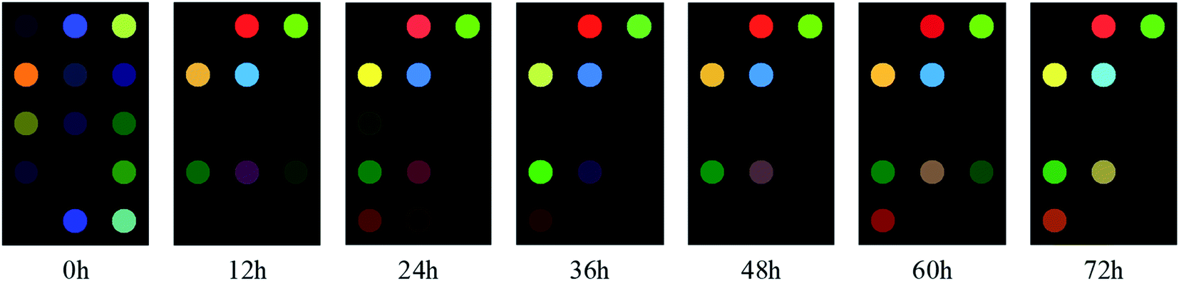Fig. 3 Difference images of colorimetric sensor for different time periods of the SSF of cassava.

3.3 Optimized reconstruction of the best combination of characteristic color components

Fig. 4 is the cumulative frequency diagram of color feature components of ACO and SA optimization algorithms after 50 runs, respectively. As can be seen clearly from the Fig. 4 that the number of times each color feature component was selected after the ACO and SA runs differed, which indicates that the random selection of the algorithm had some influence on the results. Comparing the two optimization algorithms, to ensure the accuracy of the model, the combination of feature color variables with a cumulative frequency greater than or equal to 10 times was preferred to build the model. From Fig. 4, it can be seen that there are 19 feature color components after being optimally filtered by the ACO algorithm and 21 feature color components after being optimally filtered by the SA algorithm. It can also be understood from the figure that both algorithms have selected some of the same feature color components, such as the 10th, 18th, and 30th. The appearance of these high-frequency color components indicates that the original color components are filtered by the optimization algorithm, and the high-frequency color components have better specificity for color-sensitive materials, and they are also more responsive to the changes in the constituent content of ethanol during the simultaneous saccharification and fermentation of cassava, which paves the way for the subsequent improvement of the accuracy of the quantitative model.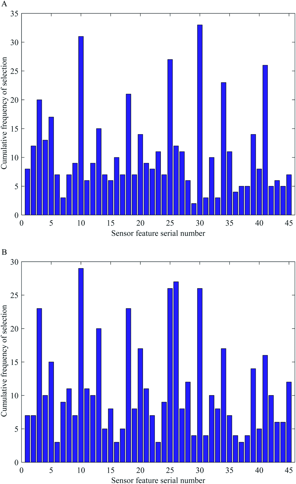

Fig. 4 Cumulative frequency of color feature components based on two different optimization algorithms. (A) Cumulative frequency plot of color feature components after 50 times of ACO algorithm runs; (B) cumulative frequency plot of color feature components after 50 times of the SA algorithm runs.

3.4 Results of the BPNN models based on the optimal characteristic color components

Table 3 shows the statistical results of the BPNN model constituted from the optimal characteristic color components obtained by running different intelligent optimization algorithms 50 times. From the Table 3, it can be seen that the BPNN models optimized based on both algorithms have mean R_C² values greater than 0.94 in the calibration set and mean R_P² values greater than 0.76 in the prediction set, which indicates that the different feature variables reconstructed by these two algorithms have better accuracy and stability in the BPNN models. At the same time, it can also be seen from the table that the root mean square error of calibration (RMSEC) and the root mean square error of prediction (RMSEP) generated by the two optimization algorithms are very close, which indicates that the optimization performance of the two algorithms is very similar in the results of variable screening, so both algorithms can be applied to the establishment of subsequent calibration model.

Table 3 Statistical results of the BPNN model constituted from the optimal characteristic color components obtained by running different intelligent optimization algorithms 50 times

Models	Calibration set		Prediction set
	RC^2	RMSEC	RP^2	RMSEP
	Average ± SD^a	Average ± SD^a	Average ± SD^a	Average ± SD^a
a The standard deviation.
ACO-BPNN	0.9483 ± 0.0254	6.6192 ± 1.8417	0.7785 ± 0.0783	14.1387 ± 2.5652
SA-BPNN	0.9459 ± 0.0248	6.7549 ± 1.7882	0.7624 ± 0.0798	14.7229 ± 2.3322

---

3.5 Results of the best SVR model

To further improve the accuracy of the model, the DE algorithm was used again to find the optimal values of the penalty parameter c and the kernel function g for the SVR model. Fig. 5 shows the convergence curves of the model optimization after running two different population intelligence optimization algorithms 50 times. From the Fig. 5, we can know that the ACO algorithm starts to converge and stabilize in the 9th run, while the SA algorithm converges slightly later than the ACO algorithm and starts to converge in the 16th run. Combining the two curves, it can be seen that the bestCost values of both intelligent algorithms show a rapid decrease first, and then a slow decrease in a certain interval of the number of runs until they finally stabilize.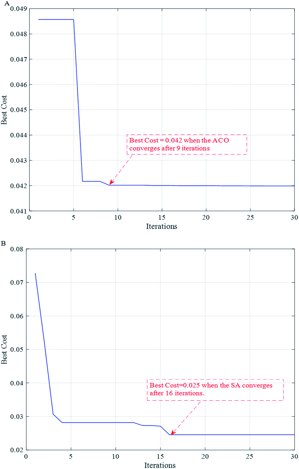

Fig. 5 Convergence curves of model optimization after running two different population intelligence optimization algorithms 50 times respectively. (A) ACO; (B) SA.

Table 4 is a statistical chart of the optimal combination results based on the SVR model. The models with input feature variables not optimized by the algorithm are labeled as combination 1; the models optimized by the ACO algorithm are labeled as combination 2; and the models optimized by the SA algorithm are labeled as combination 3. As can be seen from the Table 4, compared with the SVR model with optimized parameters c and g using the grid search method, the determination coefficients of the models with optimized SVR parameters using the DE algorithm are higher in both the calibration set and the prediction set improved than before. This indicates that using the DE algorithm in combination with the SVR model can well improve the overall accuracy of the model.

Table 4 Statistical chart of the best combination of results based on the SVR models

Type	Number of characteristic variables	Model	Parameter combinations	Calibration set		Prediction set
				RC^2	RMSEC	RP^2	RMSEP
Combination 1	45	SVR	c = 4, g = 0.0221	0.9314	0.1897	0.8606	0.2826
		DE-SVR	c = 92.2764, g = 0.01	0.9815	0.0990	0.8928	0.2392
Combination 2	19	SVR	c = 2.8284, g = 0.0884	0.9448	0.1712	0.9288	0.2011
		ACO-DE-SVR	c = 97.4921, g = 0.2097	0.9853	0.0886	0.9195	0.2049
Combination 3	21	SVR	c = 2, g = 0.0625	0.9232	0.2026	0.9280	0.2197
		SA-DE-SVR	c = 5.4241, g = 0.1265	0.9773	0.1103	0.9549	0.1562

---

Comparing combination 1, combination 2 and combination 3 again, it can be seen that: the model using the ACO and SA algorithms to optimally reconstruct the input feature variables has a higher accuracy of the coefficient of determination R_P² in the prediction set than the previous model using the original data as input. Among them, using the SA algorithm to optimize the input color feature components, combined with the DE-SVR model, can make the highest coefficient of determination R_P² in the model prediction set of 0.9549, and the corresponding root mean square error RMSEP is the lowest of 0.1562, at this time c = 5.4241, g = 0.1265. Specifically, the root mean square error of prediction (RMSEP) here is as small as possible, it is actually a kind of discrete degree, is not the absolute error, in the model represents the degree of deviation of the predicted values and the real value. It can well reflect the precision of the model, and also illustrates the pattern recognition algorithm has very good effect on the entire model.

Finally, it is concluded that in the fermentation process, an odor has hundreds of components, and it is unrealistic to measure an odor with multiple porphyrin gas sensitive points at the same time. Although the data collected by the colorimetric sensor is the result of multiple odor responses, the colorimetric sensor takes advantage of the fact that each porphyrin gas sensitive point responds to various components in the complex gas but is different from each other, and then uses a variety of data processing methods to identify the odor. Moreover, due to the application of the method of pattern classification, we are able to extract useful information from a variety of redundant information, which improves the overall sensitivity of the colorimetric sensor by several orders of magnitude. In this research, SA optimization algorithm was first used to optimize the input feature color components, and using the DE algorithm to optimize the SVR model parameters c and g, the most accurate model can be obtained for the detection of ethanol content in the fermentation process. From the establishment of the overall model, it can be seen that the model can achieve high accuracy in the detection of ethanol fermentation content, which means that in terms of algorithm, ethanol measurement also has a high sensitivity, this technology is fully feasible in the detection of ethanol content in the fermentation process. At the same time, compared to Feng et al.,²⁷ who applied the electronic nose technology to the detection of key parameters in the ethanol fermentation process, this paper is a breakthrough in using a more advanced olfactory visualization technology than the electronic nose technology, which is not only more convenient to operate the equipment than the electronic nose technology, but also presents good results as the first technology applied to ethanol measurement, which provides a theoretical reference for the application of this technology to other fields of the fermentation industry in the future. Compared with Zhang et al.,²⁸ which uses near-infrared spectroscopy technology to detect ethanol content, its prediction accuracy in the model finally reached 0.9694, which is higher than the model accuracy of this study. This also reflects from the side that olfactory visualization technology, as an emerging technology, still has a good research space, such as: how to make the data more stable collection, how to improve the composition of the olfactory system, etc.

4. Conclusions

In this study, we developed a colorimetric sensor array for the parameter detection of the SSF of cassava to achieve the quantitative detection of ethanol content in the SSF of cassava. By introducing two population intelligence algorithms, i.e. SA and ACO, to optimize the input feature variables of the SVR model, it was found that the SVR model using the algorithm-optimized input feature variables had higher accuracy than the model using the original variables. When the internal parameters c and g of the SVR model were optimized using the DE algorithm again, it was found that the input feature variables optimized using the SA algorithm achieved the best prediction accuracy of the model in the DE-SVR model run. It is concluded that the use of colorimetric sensor technique combined with different population intelligence optimization algorithms to build models can effectively meet the monitoring of ethanol content in the SSF of cassava, which has good application prospects.

Conflicts of interest

All authors declare that they have no conflict of interest.

Acknowledgements

The authors gratefully acknowledge the financial support provided by the National Natural Science Foundation of China (Grant No. 61705093), the Six Talent Peaks Project in Jiangsu Province (Grant No. NY151), and the Postgraduate Research & Practice Innovation Program of Jiangsu Province (Grant No. SJCX20_1404).

References

1. J.-Z. Zhou, J.-X. Feng, Q. Xu and Y.-J. Zhao, Renewable Energy, 2018, 123, 675–682.
2. A. Gasparatos, C. N. H. Doll, M. Esteban, A. Ahmed and T. A. Olang, Renewable Sustainable Energy Rev., 2017, 70, 161–184.
3. C. Whittaker, A. L. Borrion, L. Newnes and M. McManus, Appl. Energy, 2014, 122, 207–215.
4. M. Hans, S. Kumar, A. K. Chandel and I. Polikarpov, Process Biochem., 2019, 85, 125–134.
5. X. Shi, Y. Liu, J. Dai, X. Liu, S. Dou, L. Teng, Q. Meng, J. Lu, X. Ren and R. Wang, Biomass Bioenergy, 2019, 121, 115–121.
6. X.-w. Huang, X.-b. Zou, J.-y. Shi, Z.-h. Li and J.-w. Zhao, Trends Food Sci. Technol., 2018, 81, 90–107.
7. N. A. Rakow and K. S. Suslick, Nature, 2000, 406, 710–713.
8. K. Urmila, H. Li, Q. Chen, Z. Hui and J. Zhao, Anal. Methods, 2015, 7, 5682–5688.
9. H. Jiang, W. Xu and Q. Chen, Food Res. Int., 2019, 126, 108605.
10. Q. Chen, W. Hu, J. Su, H. Li, Q. Ouyang and J. Zhao, J. Food Eng., 2016, 168, 259–266.
11. K. S. Suslick, N. A. Rakow and A. Sen, Tetrahedron, 2004, 60, 11133–11138.
12. N. A. Gavrilenko, N. V. Saranchina and M. A. Gavrilenko, J. Anal. Chem., 2015, 70, 1475–1479.
13. M.-L. Ye, Y. Zhu, Y. Lu, L. Gan, Y. Zhang and Y.-G. Zhao, Talanta, 2021, 230, 122299.
14. S. Chen, Z. Xue, N. Gao, X. Yang and L. Zang, Sensors, 2020, 20, 917.
15. Z. Li, J. R. Askim and K. S. Suslick, Chem. Rev., 2019, 119, 231–292.
16. J.-H. Lee, J.-H. Park, H. S. Cho, S. W. Joo, M. H. Cho and J. Lee, Biofouling, 2013, 29, 491–499.
17. C. Paul and G. K. Vishwakarma, Commun. Stat. Simulat. Comput., 2017, 46, 6772–6789.
18. H. Jiang, W. Xu and Q. Chen, Sensors, 2019, 19, 2021.
19. H. Jiang and Q. Chen, Food Anal. Methods, 2015, 8, 954–962.
20. R. Lv, X. Huang, J. H. Aheto, C. Dai and X. Tian, J. Food Process Eng., 2019, 42, e13225.
21. H. Jiang, Y. He and Q. Chen, J. Sci. Food Agric., 2020, 3448–3456.
22. H. Jiang, W. D. Xu, Y. H. Ding and Q. S. Chen, Spectrochim. Acta, Part A, 2020, 228, 8.
23. S. Tabakhi, P. Moradi and F. Akhlaghian, Eng. Appl. Artif. Intell., 2014, 32, 112–123.
24. H. Jiang, W. Xu and Q. Chen, Food Chem., 2020, 319, 126584.
25. M. M. Mafarja and S. Mirjalili, Neurocomputing, 2017, 260, 302–312.
26. R. Mallipeddi, P. N. Suganthan, Q. K. Pan and M. F. Tasgetiren, Appl. Soft Comput., 2011, 11, 1679–1696.
27. Y. Feng, X. Tian, Y. Chen, Z. Wang, J. Xia, J. Qian, Y. Zhuang and J. Chu, Bioresour. Bioprocess., 2021, 8, 37.
28. G. Zhang, G. Deng, W. Wang, Q. Gu, H. Zhao and J. Zeng, Chin. J. Explos. Propellants, 2020, 43, 563–568.

---