
 Open Access Article
 This Open Access Article is licensed under a Creative Commons Attribution-Non Commercial 3.0 Unported Licence
Versailles project on advanced materials and standards (VAMAS) interlaboratory study on measuring the number concentration of colloidal gold nanoparticles†
Caterina
Minelli
 *a,
Magdalena
Wywijas‡
a,
Dorota
Bartczak
b,
Susana
Cuello-Nuñez
b,
Heidi Goenaga
Infante
b,
Jerome
Deumer
c,
Christian
Gollwitzer
c,
Michael
Krumrey
c,
Karen E.
Murphy
d,
Monique E.
Johnson
d,
Antonio R.
Montoro Bustos
d,
Ingo H.
Strenge§
d,
Bertrand
Faure
e,
Peter
Høghøj
e,
Vivian
Tong
a,
Loïc
Burr
f,
Karin
Norling
g,
Fredrik
Höök
g,
Matthias
Roesslein
h,
Jovana
Kocic
i,
Lyndsey
Hendriks¶
i,
Vikram
Kestens
j,
Yannic
Ramaye
j,
Maria C.
Contreras Lopez
j,
Guy
Auclair
j,
Dora
Mehn
k,
Douglas
Gilliland
k,
Annegret
Potthoff
l,
Kathrin
Oelschlägel||
l,
Jutta
Tentschert
m,
Harald
Jungnickel
m,
Benjamin C.
Krause
m,
Yves U.
Hachenberger
m,
Philipp
Reichardt
m,
Andreas
Luch
m,
Thomas E.
Whittaker**
n,
Molly M.
Stevens
n,
Shalini
Gupta
o,
Akash
Singh††
o,
Fang-hsin
Lin
p,
Yi-Hung
Liu
p,
Anna Luisa
Costa
q,
Carlo
Baldisserri
q,
Rid
Jawad
r,
Samir E. L.
Andaloussi
r,
Margaret N.
Holme
rn,
Tae Geol
Lee
s,
Minjeong
Kwak
s,
Jaeseok
Kim
s,
Johanna
Ziebel
t,
Cedric
Guignard
t,
Sebastien
Cambier
t,
Servane
Contal
t,
Arno C.
Gutleb
t,
Jan
“Kuba” Tatarkiewicz
u,
Bartłomiej J.
Jankiewicz
v,
Bartosz
Bartosewicz
v,
Xiaochun
Wu
w,
Jeffrey A.
Fagan
d,
Elisabeth
Elje
xy,
Elise
Rundén-Pran
x,
Maria
Dusinska
x,
Inder Preet
Kaur
z,
David
Price
aa,
Ian
Nesbitt
ab,
Sarah
O′ Reilly
ab,
Ruud J. B.
Peters
ac,
Guillaume
Bucher
ad,
Dennis
Coleman
ae,
Angela J.
Harrison
ae,
Antoine
Ghanem
af,
Anne
Gering
af,
Eileen
McCarron
ag,
Niamh
Fitzgerald
ag,
Geert
Cornelis
ah,
Jani
Tuoriniemi
ah,
Midori
Sakai
ai,
Hidehisa
Tsuchida
ai,
Ciarán
Maguire‡‡
aj,
Adriele
Prina-Mello
aj,
Alan J.
Lawlor
ak,
Jessica
Adams
ak,
Carolin L.
Schultz
al,
Doru
Constantin
am,
Nguyen Thi Kim
Thanh
an,
Le Duc
Tung
an,
Luca
Panariello§§
ao,
Spyridon
Damilos¶¶
ao,
Asterios
Gavriilidis
ao,
Iseult
Lynch
ap,
Benjamin
Fryer
ap,
Ana
Carrazco Quevedo
ap,
Emily
Guggenheim
ap,
Sophie
Briffa
ap,
Eugenia
Valsami-Jones
ap,
Yuxiong
Huang
aq,
Arturo A.
Keller
aq,
Virva-Tuuli
Kinnunen
ar,
Siiri
Perämäki
ar,
Zeljka
Krpetic
as,
Michael
Greenwood
as and
Alexander G.
Shard
a
*a,
Magdalena
Wywijas‡
a,
Dorota
Bartczak
b,
Susana
Cuello-Nuñez
b,
Heidi Goenaga
Infante
b,
Jerome
Deumer
c,
Christian
Gollwitzer
c,
Michael
Krumrey
c,
Karen E.
Murphy
d,
Monique E.
Johnson
d,
Antonio R.
Montoro Bustos
d,
Ingo H.
Strenge§
d,
Bertrand
Faure
e,
Peter
Høghøj
e,
Vivian
Tong
a,
Loïc
Burr
f,
Karin
Norling
g,
Fredrik
Höök
g,
Matthias
Roesslein
h,
Jovana
Kocic
i,
Lyndsey
Hendriks¶
i,
Vikram
Kestens
j,
Yannic
Ramaye
j,
Maria C.
Contreras Lopez
j,
Guy
Auclair
j,
Dora
Mehn
k,
Douglas
Gilliland
k,
Annegret
Potthoff
l,
Kathrin
Oelschlägel||
l,
Jutta
Tentschert
m,
Harald
Jungnickel
m,
Benjamin C.
Krause
m,
Yves U.
Hachenberger
m,
Philipp
Reichardt
m,
Andreas
Luch
m,
Thomas E.
Whittaker**
n,
Molly M.
Stevens
n,
Shalini
Gupta
o,
Akash
Singh††
o,
Fang-hsin
Lin
p,
Yi-Hung
Liu
p,
Anna Luisa
Costa
q,
Carlo
Baldisserri
q,
Rid
Jawad
r,
Samir E. L.
Andaloussi
r,
Margaret N.
Holme
rn,
Tae Geol
Lee
s,
Minjeong
Kwak
s,
Jaeseok
Kim
s,
Johanna
Ziebel
t,
Cedric
Guignard
t,
Sebastien
Cambier
t,
Servane
Contal
t,
Arno C.
Gutleb
t,
Jan
“Kuba” Tatarkiewicz
u,
Bartłomiej J.
Jankiewicz
v,
Bartosz
Bartosewicz
v,
Xiaochun
Wu
w,
Jeffrey A.
Fagan
d,
Elisabeth
Elje
xy,
Elise
Rundén-Pran
x,
Maria
Dusinska
x,
Inder Preet
Kaur
z,
David
Price
aa,
Ian
Nesbitt
ab,
Sarah
O′ Reilly
ab,
Ruud J. B.
Peters
ac,
Guillaume
Bucher
ad,
Dennis
Coleman
ae,
Angela J.
Harrison
ae,
Antoine
Ghanem
af,
Anne
Gering
af,
Eileen
McCarron
ag,
Niamh
Fitzgerald
ag,
Geert
Cornelis
ah,
Jani
Tuoriniemi
ah,
Midori
Sakai
ai,
Hidehisa
Tsuchida
ai,
Ciarán
Maguire‡‡
aj,
Adriele
Prina-Mello
aj,
Alan J.
Lawlor
ak,
Jessica
Adams
ak,
Carolin L.
Schultz
al,
Doru
Constantin
am,
Nguyen Thi Kim
Thanh
an,
Le Duc
Tung
an,
Luca
Panariello§§
ao,
Spyridon
Damilos¶¶
ao,
Asterios
Gavriilidis
ao,
Iseult
Lynch
ap,
Benjamin
Fryer
ap,
Ana
Carrazco Quevedo
ap,
Emily
Guggenheim
ap,
Sophie
Briffa
ap,
Eugenia
Valsami-Jones
ap,
Yuxiong
Huang
aq,
Arturo A.
Keller
aq,
Virva-Tuuli
Kinnunen
ar,
Siiri
Perämäki
ar,
Zeljka
Krpetic
as,
Michael
Greenwood
as and
Alexander G.
Shard
a
aChemical & Biological Sciences Department, National Physical Laboratory, Hampton Road, Teddington TW11 0LW, UK. E-mail: caterina.minelli@npl.co.uk
bNational Measurement Laboratory, Queens road, Teddington TW11 0LY, UK
cPhysikalisch-Technische Bundesanstalt (PTB), Abbestr. 2-12, 10587 Berlin, Germany
dNational Institute of Standards and Technology, 100 Bureau Drive, Gaithersburg, Maryland 20899-8391, USA
eXenocs SAS, 1-3 Allée du Nanomètre, 38000 Grenoble, France
fCSEM SA, Bahnhofstrasse 1, 7242 Landquart, Switzerland
gChalmers University of Technology, Gothenburg 412 96, Sweden
hEmpa, Swiss Federal Laboratories for Material Science and Technology, Lerchenfeldstrasse 5, CH-9014 St Gallen, Switzerland
iETH Zurich, Vladimir-Prelog-Weg 1, 8093 Zurich, Switzerland
jEuropean Commission, Joint Research Centre (JRC), Geel, Belgium
kEuropean Commission, Joint Research Centre (JRC), Ispra, Italy
lFraunhofer Institute for Ceramic Technologies and Systems IKTS, Winterbergstr. 28, 01217 Dresden, Germany
mThe German Federal Institute for Risk Assessment, Max-Dohrn Str. 8-10, Berlin, Germany
nDepartment of Materials, Department of Bioengineering and Institute of Biomedical Engineering, Imperial College London, Exhibition road, London SW7 2BX, UK
oIndian Institute of Technology Delhi, New Delhi 110016, India
pCentre for Measurement Standards, Industrial Technology Research Institute, No. 321, Sec. 2, Kuang Fu Rd., Hsinchu, 30011, Taiwan, Republic of China
qInstitute of Science and Technology for Ceramics, Via Granarolo 64, 48018 Faenza, Italy
rKarolinska Institutet, 171 77 Stockholm, Sweden
sKorea Research Institute of Standards and Science (KRISS), 267 Gajeong-ro, Yuseong-gu, Daejeon 34113, Korea
tLuxembourg Institute of Science and Technology, 41 rue du Brill, L-4422 Belvaux, Luxembourg
uMANTA Instruments, Inc., San Diego, CA, USA
vMilitary University of Technology, gen. Sylwestra Kaliskiego 2 str., 00-908 Warsaw, Poland
wNational Center for Nanoscience and Technology (NCNST), No. 11, ZhongGuanCun BeiYiTiao, Beijing 100190, People's Republic of China
xNILU—Norwegian Institute for Air Research, Instituttveien 18, 2007 Kjeller, Norway
yUniversity of Oslo, Sognsvannsveien 9, 0372 Oslo, Norway
zNottingham Trent University, 50 Shakespeare St, Nottingham NG1 4FQ, UK
aaPerkinElmer, Chalfont Road, Seer Green, Bucks HP92FX, UK
abPublic Analyst's Laboratory, Sir Patrick Duns, Lower Grand Canal Street, Dublin 2, D02 P667, Ireland
acWageningen Food Safety Research, Wageningen University & Research, Akkermaalsbos 2, 6708 WB Wageningen, The Netherlands
adService Commun des Laboratoires, 3 Avenue Dr Albert Schweitzer, 33600 Pessac, France
aeSmith+Nephew, 101 Hessle Road, Hull HU3 2BN, UK
afSOLVAY Research & Innovation, Brussels Centre, Rue de Ransbeek 310, 1120 Brussels, Belgium
agState Laboratory, Backweston Campus, Young's Cross, Celbridge, Co Kildare, W23 VW2C, Ireland
ahSwedish University of Agricultural Sciences, Lennart Hjelms väg 9, 75651 Uppsala, Sweden
aiToray Research Center, Inc., 3-3-7 Sonoyama, Otsu, Shiga 5208567, Japan
ajTrinity Translational Medicine Institute, Trinity College Dublin, Dublin, Ireland
akUK centre for Ecology and Hydrology, Lancaster Environment Centre, Library Avenue, Bailrigg, Lancaster LA1 4AP, UK
alUK Centre for Ecology and Hydrology, Maclean Building, Benson Lane, Crowmarsh-Gifford, Wallingford, OX10 8BB, UK
amLaboratoire de Physique des Solides, Université Paris-Saclay, CNRS, 91405 Orsay, France
anDepartment of Physics and Astronomy, University College London, Gower Street, London WC1E 6BT, UK
aoDepartment of Chemical Engineering, University College London, Torrington Place, London, WC1E 7JE, UK
apSchool of Geography, Earth and Environmental Sciences, University of Birmingham, Edgbaston, B15 2TT Birmingham, UK
aqBren School of Environmental Science and Management, University of California at Santa Barbara, CA 93106, USA
arDepartment of Chemistry, University of Jyväskylä, P.O. Box 35, FI-40014 Jyväskylä, Finland
asSchool of Science Engineering and Environment, University of Salford, M5 4WT Salford, UK
First published on 9th March 2022
Abstract
We describe the outcome of a large international interlaboratory study of the measurement of particle number concentration of colloidal nanoparticles, project 10 of the technical working area 34, “Nanoparticle Populations” of the Versailles Project on Advanced Materials and Standards (VAMAS). A total of 50 laboratories delivered results for the number concentration of 30 nm gold colloidal nanoparticles measured using particle tracking analysis (PTA), single particle inductively coupled plasma mass spectrometry (spICP-MS), ultraviolet-visible (UV-Vis) light spectroscopy, centrifugal liquid sedimentation (CLS) and small angle X-ray scattering (SAXS). The study provides quantitative data to evaluate the repeatability of these methods and their reproducibility in the measurement of number concentration of model nanoparticle systems following a common measurement protocol. We find that the population-averaging methods of SAXS, CLS and UV-Vis have high measurement repeatability and reproducibility, with between-labs variability of 2.6%, 11% and 1.4% respectively. However, results may be significantly biased for reasons including inaccurate material properties whose values are used to compute the number concentration. Particle-counting method results are less reproducibile than population-averaging methods, with measured between-labs variability of 68% and 46% for PTA and spICP-MS respectively. This study provides the stakeholder community with important comparative data to underpin measurement reproducibility and method validation for number concentration of nanoparticles.
Introduction
The advancement of analytical methods for nanoparticle measurements is critical both for the growing industrial exploitation of engineered nanoparticles and for developing robust strategies to understand and control the concentration of nanomaterials in humans and the environment.For high value nanoparticles, the measurement of nanoparticle number concentration in a liquid directly impacts the ability to assess the scale and reproducibility of the production process, it allows optimisation of efficiency and supports regulatory compliance. This measurement is also useful to monitor and control the intentional or accidental release of engineered nanoparticles into the environment at the production plant, as well as by end-users.1–3
From a metrological point of view, the measurement of the number concentration of nanoscale particles is challenging due to technological limitations, and a lack of validated measurement protocols and reference materials for calibration, quality control and establishing metrological traceability. Combined, these factors contribute to the inability of laboratories to assess method performance, for example in terms of measurement accuracy, reproducibility and result comparability. Thanks to a number of international efforts in recent years, this situation is improving.2–12 Documentary standards have been developed within the International Organization for Standardisation (ISO) for a number of techniques capable of performing number concentration measurements including population-averaging methods such as: small angle X-ray scattering (SAXS),13 dynamic light scattering14,15 and centrifugal liquid sedimentation (CLS),16,17 as well as particle-counting methods such as, single particle inductively coupled plasma mass spectrometry (spICP-MS),18 particle tracking analysis (PTA),19 differential mobility analysis with integrated condensation particle counter20 and resistive pulse sensing (RPS).21 Many of these standards, however, describe aspects of particle size analysis rather than measurement of number concentration. As such, an ISO technical report providing guidance on the measurement of number concentration is being developed in ISO TC 229, the technical committee on nanotechnologies.22 Within the European project 14IND12 Innanopart of the European Metrology Programme for Innovation and Research (EMPIR), it was demonstrated that of the above-listed techniques, both SAXS and spICP-MS measure the colloidal number concentration with a relative expanded uncertainty better than 10% and that both methods yield results that are directly traceable to the relevant units of the International System of Units (SI).6 Utilizing spICP-MS and the so-called dynamic mass flow (DMF) approach to calibrate the mass of the particle suspension transported into the plasma, the first quality control (QC) material, LGCQC5050, with an assigned nanoparticle number concentration value that is traceable to the SI unit for mass (kilogram) was released in 2019 by LGC.12,23 Prior to the assignment of the number concentration value by LGC, this material was used as basis for the interlaboratory study reported here.
In this work, we undertook a large international interlaboratory comparison of five measurement methods for number-based particle concentration of colloidal gold suspensions under the umbrella of the Versailles Project on Advanced Materials and Standards (VAMAS), namely project 10 of the VAMAS technical working area (TWA) 34 (Nanoparticle Populations). VAMAS is an international organisation that supports world trade in products dependent on advanced materials technologies, through international collaborative projects aimed at providing the technical basis for harmonised measurements, testing, specifications, and standards. The lead organisation, the UK National Physical Laboratory, provided 54 laboratories across the world with colloidal gold nanoparticle samples, together with a common measurement protocol24 and a reporting form in October 2017. Results were collected largely during the year 2018, but additional results were accepted up until 2021. To ensure comparability of results amongst the participants, all laboratories were asked to adhere to the provided instructions for sample storage and preparation. Prior to sample shipment to the participants, the supplied material was assessed for its between-unit homogeneity by LGC and its storage stability was monitored for the duration of the study. Different techniques were employed by participants, namely spICP-MS, PTA, ultraviolet-visible (UV-Vis) spectroscopy,11,25 CLS and SAXS. The aim of the study was two-fold. Primarily, the study sought to assess and compare method reproducibility amongst different laboratories. Secondarily, the study aimed to establish best practices in the use of the various techniques for determination of particle number concentration and the related sample preparation procedures.
Interlaboratory study details
Sample
The selection and preparation of the nanoparticle materials for the study were pivotal to a successful outcome in the comparison. Candidate materials were examined and tested within the EMPIR project Innanopart (2015–2018), including near-spherical gold, silica and polystyrene colloids with nominal diameters between 5 nm and 500 nm. Citrate-stabilised 30 nm colloidal gold particles from BBI Solutions (Newport, UK) was selected as source material due to its performance in terms of sample stability evaluations.The test materials for the study had an average core size of 30.7 nm according to manufacturer's information. The size distribution was measured by CLS and spICP-MS and results are reported in section S1 of the ESI.† Representative SEM images of the particles are also shown in Fig. S3 of the ESI.† The test materials consisted of aqueous suspensions of near-spherical colloidal gold nanoparticles with a nominal diameter of 30 nm. These were ampouled and packaged by the LGC's facilities in Luckenwalde, Germany, as 5 mL vials labelled with full number and value assigned for number concentration by the NML at LGC in Teddington, UK. The vials were sterilised using Co60 gamma-irradiation with a minimum dose of 35 kGy and homogeneity and stability studies were performed by PTA at LGC (Teddington, UK, see the Certificate of Analysis for more details on homogeneity and stability assessment23) to ensure the product was consistent and stable for the entire duration of the study. Each laboratory was supplied with 5 ampoules. It was recommended that the content of each ampoule was used within a day from opening. An indication of the value for the colloidal gold number concentration between 1014 kg−1 and 1015 kg−1 was provided to the participants, but not the accepted reference value.
The reference value of the number concentration of the colloidal gold test sample, used for comparability purposes of the results obtained under the VAMAS study reported here, was determined by LGC through characterisation of the same material independently of this study using spICP-MS with DMF approach for the transport efficiency determination.12 The assessed value ((1.47 ± 0.28) × 1014 kg−1, with a 95% confidence level),23 was measured with an ICP-MS instrument equipped with a conventional MicroMist nebuliser and a Scott-type spray chamber cooled to 2 °C.
Measurement protocol
Both electronic and paper versions of the measurement protocol were provided to all participants to the study together with the samples. The protocol was authored by a team of scientists at NPL and LGC and published as the NPL Report AS 98.24 The report is publicly available and a copy of it is in section S2 of the ESI.† The protocol contains recommendations on how to handle and prepare the samples, how to prepare gravimetric dilutions and how to perform the measurements by UV-Vis, CLS, PTA and spICP-MS. An electronic reporting spreadsheet was provided to all participants, which was designed to compile these details together with the measurement results.Importantly, because different methods require different degrees of sample dilution, a robust dilution protocol is crucial for reproducible and comparable number concentration results. The accuracy of the dilution factor directly impacts the measurement of the number concentration of the sample. For this reason, care was taken in developing consistent protocols for sample dilution and part of the study was devoted to raise awareness of the different approaches to dilution and disseminate best practice. To this end, all participants were requested to perform some dilutions. For those participants using particle-counting methods, spICP-MS and PTA, the dilution was necessary to meet optimum sample analysis conditions. For the particle-averaging methods, SAXS, UV-Vis spectroscopy and CLS, the concentration of the sample provided was compatible with the methods and dilution was not necessary. Three out of the five sample vials were measured as provided (sample NPL1). However, the participants were also requested to dilute the suspensions in the remaining vials by a factor of about 5 (sample NPL2) and 10 respectively and measure the number concentration of the resulting suspensions. For NPL1, measurements were repeated on at least three independent aliquots, each one from one of the three vials provided. For NPL2 and NPL3, measurements were performed on at least three different aliquots for each sample. This enabled an evaluation of the impact of sample dilution on measurement performance and offered an opportunity to the various participating laboratories to assess the available equipment and practices and address any identified inconsistencies.
The provided protocol was not compulsory, but the participants were requested to document any deviation from it to ensure the history of each sub-sample was known. The protocol recommended performing the sample dilutions gravimetrically, i.e. through the aid of an analytical balance. Pipettes were typically used to transfer the sample and the diluent, which was either ultrapure water (resistivity of 18.2 MΩ cm at 25 °C) or filtered citrate buffer, but it was recommended to place the vials on the plate of a balance, wherein the variations in weights due to the addition of liquid were recorded. Assuming that the balance was calibrated and well maintained, this permits measurement of the dilution factor with a relative accuracy of the order of 0.1%, well below the typical uncertainty associated with particle number concentration measurements using currently available techniques. This means that the uncertainty component arising from the sample dilution is practically negligible. Where dilutions were prepared volumetrically, i.e. with the use of the pipettes only, the accuracy of the dilution factor relies on the pipette calibration, the temperature of the liquid being measured and the skills of the operator. For particle-counting methods, which require higher dilution factors with respect to population-average methods, it was recommended to use filtered 1 mM citrated buffer as a dispersant to minimise the risk of sample instability.
For the methods of UV-Vis spectroscopy, CLS, PTA and spICP-MS, the measurement protocol also provided recommendations on calibration strategies, instrument settings and data handling. Some experimental details are briefly described below for each of the methods.
SAXS
SAXS is a well-established technique to characterise nanoparticle suspensions. It is based on the scattering of X-rays under small angles in forward direction.26 The scattering signal is proportional to: the number of scatterers in the illuminated volume, and thus the number concentration, the square of the effective electron density difference between the particles and the suspending medium, and the 6th power of the particle radius. It is therefore mandatory to determine the electron density contrast, e.g. by prior knowledge of the chemical composition, its molar mass and mass density of the particles and the medium, and the particle size, which for colloidal gold nanoparticles, like the ones used in this study, can be determined from the scattering curve itself with very high accuracy. For particles composed of metallic gold, the electron contrast can be calculated under the assumption that the particles have the same density as bulk gold. Since scattering and absorption cross sections of atoms depend also on the incident photon energy, the electron contrast is a function of the photon energy which must be considered by applying the known atomic scattering factors during SAXS data evaluation.27,28 Neglecting this energy-dependence may eventually lead to false results of the number concentration. Prior to SAXS data evaluation, the measured scattering signal must be normalized by several experimental parameters which are simultaneously measured, such as the incident photon flux, the sample's transmission, or the quantum efficiency of the detector's pixels. An uncertainty budget comprising all essential experimental parameters has been demonstrated leading to a relative expanded uncertainty of the evaluated number concentration of <7%,6 thus making SAXS an accurate and traceable method in determining number concentrations.Excellent reproducibility of the SAXS method has been demonstrated in previous interlaboratory comparisons29,30 and for this reason the VAMAS study only included two laboratories that performed SAXS measurements.
CLS
CLS techniques quantify the separation of colloidal particles from a liquid under the presence of a centrifugal force. The particle migratory motion (settling) occurs in presence of a density contrast between the particles and the liquid. The driving force for the particle motion is the centrifugal force, which is opposed by the drag force. As a result, the settling velocity depends on particle characteristics such as size, density and shape. CLS instruments consist of either disc or cuvette centrifuges. However, all reports submitted to this study involved the use of a disc centrifuge, in which case the method is also known as differential centrifugal sedimentation (DCS). In these types of instruments,31 the sample is injected at the centre of the disc and sediments towards the edge. Its light extinction is detected close to the edge of the disc where a laser diode and a photodetector are aligned at opposite sides of the disc. Using Stokes' law and assumptions on the particle density and spherical geometry, light extinction-based particle size distributions are generated and converted to particle mass-based distributions using Mie light scattering theory. Participants were requested to report the experimental settings selected for the measurements and to record results assuming an effective particle density of 15.0 g cm−3. We note that this value differs from that of gold's bulk density and is only valid for particles with the same size and shape as those used in this work. Reasons for this include that the value takes account of all the material enclosed within the particles Stokes volume, which also comprises citrate and solvent molecules bound and adsorbed at the surface of the gold particle. Participants were also instructed to weigh the syringe before and after each injection as to determine the mass of the injected dispersion. Presented results are normalised to the injection volume.UV-Vis spectroscopy
UV-Vis spectroscopy measures the relative intensity of a monochromatic beam light passing through a sample for a range of radiation wavelengths. Particle number concentration is derived from the light absorption according to Beer–Lambert law and Mie theory.11 Absorption spectra at wavelengths between 390 nm and 700 nm were acquired in triplicate with increments of 1 nm. Average absorption at 450 nm was ultimately chosen for the measurement of the particle number concentration, together with a recommended molar extinction coefficient of (2.16 ± 0.12) × 109 M−1 cm−1.PTA
In PTA, a diluted suspension of nanoparticles is illuminated with a laser light and the light scattered by individual particles is visualised with an optical microscope and recorded over time. The equivalent spherical hydrodynamic diameter of individual particles is determined by tracking them over time and measuring their translational diffusion coefficient, while the number concentration results from counting the particles in a known volume. Participants were requested to dilute the five samples provided and perform 5 independent measurements, one for each vial. For each measurement, participants were instructed to prepare several aliquots according to their in-house procedure and acquire a minimum of 5 independent videos of 60 seconds for each aliquot under repeatability conditions. It was recommended to analyse a QC material at the beginning, in the middle and at the end of each measurement session. Because QC materials were not provided for the study, the participants who performed such measurements were asked to identify suitable materials and record relevant information.spICP-MS
In spICP-MS, a diluted sample is introduced into the ICP-MS instrument at a set flow rate. A plasma atomises and ionises the particles producing an ion cloud for detection by mass spectrometry. The technique works by acquiring individual intensity readings with very short dwell times to ensure that signals from single particles can be resolved. With most current instrumentations, typical dwell times between 50 μs and 10 ms are used. To satisfy the single particle rule, the number of detected peaks should not exceed 10% of the maximum number of possible events per minute. As an example, using a dwell time of 3 ms, a maximum of 20![[thin space (1/6-em)]](https://www.rsc.org/images/entities/char_2009.gif) 000 particles can be registered per minute, but it is recommended that the number of pulses in the time scan does not exceed ≈1200 per minute.32,33 The overall number of peaks detected per minute is directly proportional to the number of particles in the suspension. Participants were requested to dilute the five samples and perform 5 independent measurements, one for each vial. For each measurement, participants were instructed to prepare a number of aliquots according to their in-house procedure and acquire a minimum of 5 measurement replicates of 60 s scan duration per aliquot under repeatability conditions. In addition, participants were requested to determine the instrument transport efficiency by following the in-house practice, possibly at the start, middle and at the end of the measurement session to be able to assess the variability of this parameter. A known drawback in ICP-MS is the incomplete transport of solution from the nebulizer into the plasma. Consequently, the transport efficiency of the system needs to be determined in order to accurately equate the number of detected nanoparticles to the number concentration of the original sample. Several approaches exist,34,35 but none was specifically recommended against the local laboratory practice. The participants were requested to measure a QC material at the beginning, in the middle and at the end of each measurement session. Because no such materials were provided for the study, the participants who performed such measurements were asked to identify suitable materials and record relevant information.
000 particles can be registered per minute, but it is recommended that the number of pulses in the time scan does not exceed ≈1200 per minute.32,33 The overall number of peaks detected per minute is directly proportional to the number of particles in the suspension. Participants were requested to dilute the five samples and perform 5 independent measurements, one for each vial. For each measurement, participants were instructed to prepare a number of aliquots according to their in-house procedure and acquire a minimum of 5 measurement replicates of 60 s scan duration per aliquot under repeatability conditions. In addition, participants were requested to determine the instrument transport efficiency by following the in-house practice, possibly at the start, middle and at the end of the measurement session to be able to assess the variability of this parameter. A known drawback in ICP-MS is the incomplete transport of solution from the nebulizer into the plasma. Consequently, the transport efficiency of the system needs to be determined in order to accurately equate the number of detected nanoparticles to the number concentration of the original sample. Several approaches exist,34,35 but none was specifically recommended against the local laboratory practice. The participants were requested to measure a QC material at the beginning, in the middle and at the end of each measurement session. Because no such materials were provided for the study, the participants who performed such measurements were asked to identify suitable materials and record relevant information.
Uncertainties
All results are expressed as average values and relative or absolute standard deviations (n = 1). As such, reported errors do not include a full uncertainty budget for the various methods.Units
There are a number of measurement units that are commonly used to describe the number concentration of nanoparticles. These vary from the inverse of a volume, expressed in either litres (L) or cubic metres (m3) and their sub-units, to the inverse of a mass, expressed in kilograms (kg). The choice often depends on the method that is used to measure such concentration and whether the volume or the mass of the initial dispersion is measured. Measuring the mass of the initial dispersion is straightforward and can be executed with excellent accuracy with a calibrated laboratory balance. Furthermore, gravimetric dilutions of the dispersions, where required, can be performed while preserving good accuracy. For these reasons, in this work we took the approach of measuring the number concentration of nanoparticles in the units kg−1, but units of volume are also valid. Conversion from units of volume to unit of mass requires some assumption on the density of the dispersion. In many practical applications, including the sample we provided, the mass of the dispersed nanoparticles is negligible with respect to that of the dispersion media for the level of accuracy we can currently achieve in the measurement of the number concentration of nanoparticles.4,6,11,12 In this case, the density of the dispersion can be approximated to that of the dispersant.Participants
A total of 54 laboratories enrolled in the study, 50 of which submitted a total of 74 measurement reports, making this one of the largest VAMAS studies to date. The significant interest received by the study is a testimony to the need within the community for guidance on measurement of number concentration of nanoparticles. Fig. 1A and B provide information on the background and geographical spread of the laboratories respectively. These included national measurement institutes (NMIs), academic institutions, research organisations, instrument manufacturers, measurement service providers and industrial laboratories. 77% of the laboratories were located in Europe, but participation came from all five continents. As shown in Fig. 1c, the split among the techniques was: 3% SAXS (2 reports), 11% CLS (8 reports), 35% UV-Vis (26 reports), 24% spICP-MS (18 reports) and 27% PTA (20 reports).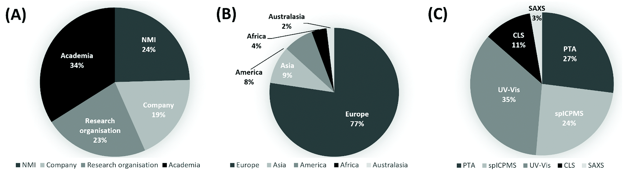 | ||
| Fig. 1 (A) Background and (B) geographical spread of the laboratories enrolled to the study. (C) Methods used by the of the laboratories contributing to the VAMAS TWA34 Project 10. | ||
Disclaimer
Certain trade names and company products are mentioned in the text or identified in illustrations in order to specify adequately the experimental procedure and equipment used. In no case does such identification imply recommendation or endorsement by the authors, nor does it imply that the products are necessarily the best available for the purpose.Results
We describe in this section the results collected within this interlaboratory comparison in terms of measurement repeatability and reproducibility. These are expressed in terms of in-lab variability, or repeatability standard deviation, and between-labs variability, or reproducibility standard deviation. The bias with respect to the accepted reference value of the number concentration of the test material, i.e. (1.47 ± 0.28) × 1014 kg−1, was also evaluated.23 Definitions of these terms are found in section S3 of the ESI.†Population-averaging methods: SAXS
SAXS measurements were performed by two laboratories, L44 and L45, as shown in Table 1. The instrumentations utilised by the two laboratories were significantly different, one using X-rays from a synchrotron radiation facility (L45) and the other one using a commercial instrument (L44). L45 used two silicon diodes (one in front and one behind the sample) to normalize the measured SAXS signal by the incoming photon flux to get the measured signal in absolute units, while L44 used the automatic normalization of the instrument, based on the simultaneous measurement of the transmitted intensity. L45 used a model fitting approach to convert the measured scattering intensities into number concentration, whereas L44 used an approach based on the Expectation Maximization algorithm36,37 to determine the number-based size distribution histogram.| Laboratory code | X-ray source | Photon energy (keV) | Beam size (mm2) | Detector | Pixel size (μm) | Type of sample holder | Sample thickness (mm) | Sample-detector distance (mm) |
|---|---|---|---|---|---|---|---|---|
| L44 | Sealed tube | 8.04 ± 0.02 | 0.8 × 0.8 | Hybrid-pixel PILATUS 200k | 172 | Glass flow cell | 1.4 | 938 |
| L45 | Synchrotron radiation (bending magnet) | 8.0000 ± 0.0008 | 0.5 × 0.5 | Hybrid-pixel PILATUS 1M | 172 | Glass capillary | 1 | 4616.3 ± 0.6 |
Taking the energy-dependence of the electron density contrast into account, the mean concentration values for SAXS resulted in 1.33 × 10¹⁴ kg−1 (L45) and 1.38 × 10¹⁴ kg−1 (L44), which deviated from the reference value by 9.5% (L45) and 6.1% (L44) respectively. Despite differences in the experimental set-up and the evaluation procedure, the resulting average number concentration values were within 3%, with a measurement repeatability standard deviation of 5% of the undiluted samples for both laboratories (Fig. 2A). The 3% difference can be explained by experimental uncertainties, or differences of the number concentration of the samples respectively. Both laboratories used a different method to analyse the scattering data, which may also cause some variations in the concentration values.
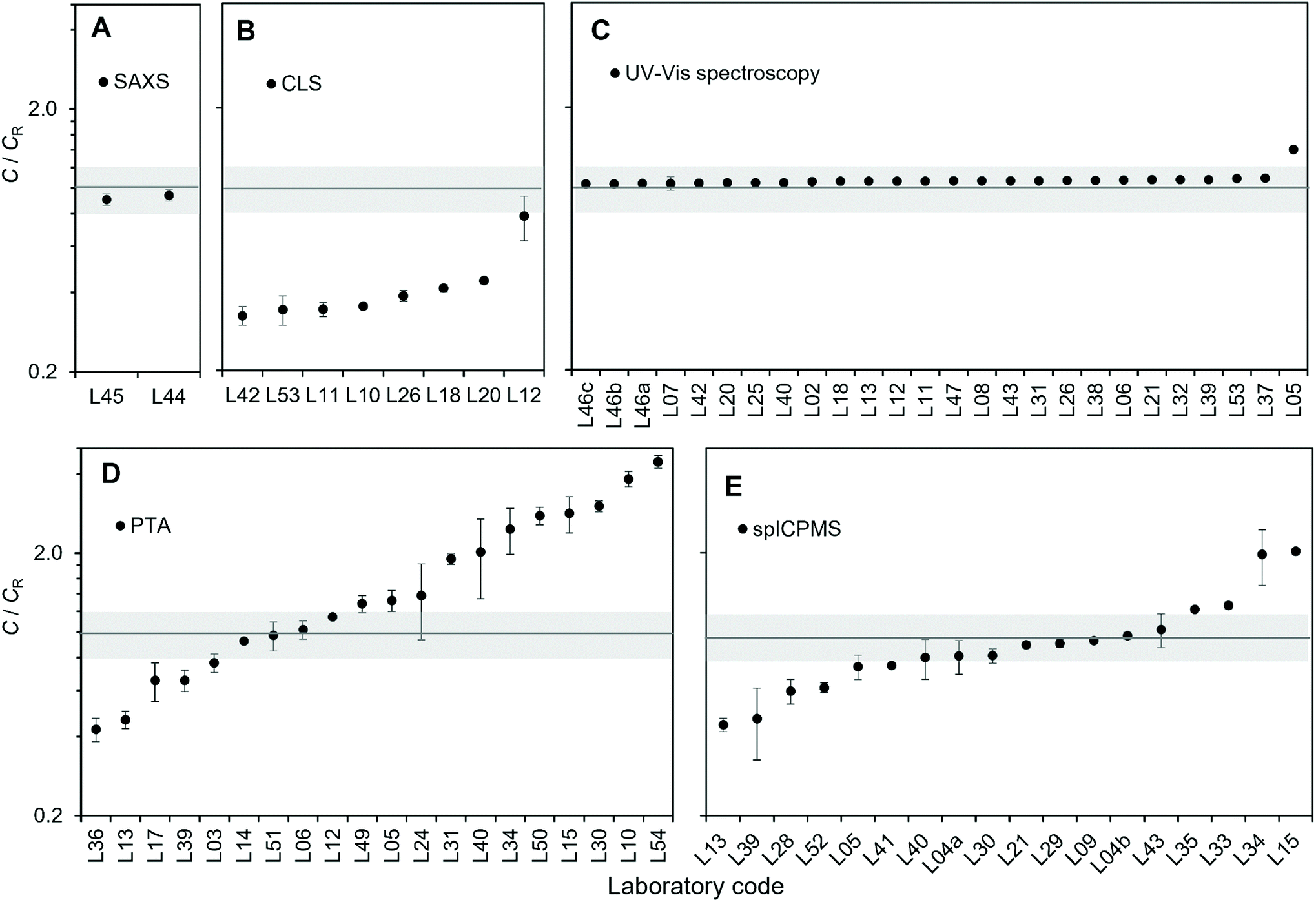 | ||
| Fig. 2 Results of the number concentration C of the test material as measured by the laboratories participating in the study by the methods of (A) SAXS, (B) CLS, (C) UV-Vis spectroscopy, (D) PTA and (E) spICP-MS expressed relative to the accepted number concentration reference value CR. The X-axis shows the laboratory codes. Error bars show the repeatability standard deviation (in-lab variability). The grey box shows the 95% confidence interval of the assigned reference value for the number concentration of the test material. | ||
Population-averaging methods: CLS
Eight laboratories delivered CLS measurement results of the undiluted sample, while seven from 5-fold and 10-fold gravimetrically prepared dilutions (Table 2). Results for the undiluted samples are shown in Fig. 2B. Because all the analytical centrifuge instruments utilised in the study were from the same manufacturer, the output data from each laboratory had the same format. It was then possible to analyse the raw data provided by all the participants by adopting the exact same analytical protocol. This has the potential advantage of minimising variability introduced by the individual laboratory analytical approaches, for example different ways of measuring the area under the peaks of the weight-based particle size distribution. However, method reproducibility did not significantly improve, indicating that the protocol for the data analysis adopted by each laboratory was robust in the first place. In terms of measurement repeatability, the average in-lab variability for the measurements of particle number concentration was 5%, excluding data from laboratory L12, which reported a repeatability standard deviation of 19%. Laboratory L12 measured a concentration twice that of the other laboratories, but the reason for this discrepancy was not identified. Specifically, the integrated particle mass was twice than that measured by the other laboratories. If we exclude L12, the between-labs variability for the measurement of the particle number concentration is 11%. In comparison, the reproducibility standard deviation for measurement of the modal value of the mass-based size distribution was better than 7%. The CLS method yielded number concentration results that were significantly below the assigned reference value. There are a number of potential reasons for this. One possibility is that particle losses occur between the injection and the detection of the particles, for example due to the particles being trapped at the surface of the fluid or adhering to the walls of the disc. In addition to this, the accuracy of the method depends on correct material properties used to calculate the concentration, the most critical parameters being the complex refractive index of both the particle materials and the fluid, but also including the particle shape and heterogeneity.| Laboratory code | Gravimetric dilutions | Instrument model and laser wavelength | Calibrant | Rotational speed (rpm) | Sucrose temperature before and after injection (°C) |
|---|---|---|---|---|---|
| a n.r. = not recorded. | |||||
| L10 | Yes | CPS Instruments DC24000 UHR, 405 nm | 264 nm PVC, CPS Instruments Lot#123 | 20000 |
n.r.a–31.5 |
| L11 | Yes | CPS Instruments DC24000 UHR, 405 nm | 237 nm PVC, CPS Instruments Lot#150 | 18000 |
24.9–34.9 |
| L12 | Yes | CPS Instruments DC24000 UHR, 405 nm | 237 nm PVC, CPS Instruments Lot#150 | 24000 |
23.6–29.1 |
| L18 | Yes | CPS Instruments DC24000 UHR, 405 nm | 145 nm silica, CPS Instruments Lot#148 | 20065 |
21.0–26.5 |
| L20 | Yes | CPS Instruments DC24000 UHR, 405 nm | 145 nm silica, China University of Petroleum, Lot#GBW(E)120059 | 20000 |
16.6–16.6 |
| L26 | Yes | CPS Instruments DC24000 UHR, 405 nm | 237 nm PVC, CPS Instruments Lot#105 | 24000 |
20.7–33.9 |
| L42 | n.a. | CPS Instruments DC24000 UHR, 405 nm | 476 nm PVC, Analytik UK | 20000 |
n.r. |
| L53 | Yes | CPS Instruments DC24000 UHR, 405 nm | 179 nm silica, nanoComposix, Lot#JEAO224 | 24000 |
28.0–37.6 |
Population-averaging methods: UV-Vis spectroscopy
Twenty-three laboratories participating in the study performed measurements using the UV-Vis method. Samples were measured both undiluted and diluted by a factor 5 and 10 (Table 3). Most laboratories performed gravimetric dilutions, except for three participants who used volumetric dilutions. Results for the undiluted samples are shown in Fig. 2C. The average measurement repeatability within each laboratory was excellent with repeatability standard deviations below 0.5%. Excluding laboratory L05, between-labs variability was of 1.4%. Laboratory L05 detected problems in the instrument photometer shortly after the study and it is likely that these problems were also present at the time of the study.| Laboratory code | Gravimetric dilutions | Instrument model and light source | Cuvette | Temperature (°C) |
|---|---|---|---|---|
| L02 | Yes | Analytik Jena Specord Plus 200, deuterium/halogen, dual beam | Brandt 759081D, PMMA, 1 cm, 2.5 mL | Room temp. |
| L05 | Yes | Varian Cary 50 Bio, xenon, dual beam | Ratiolab 2712120, PS, 1 cm, 1 mL | 20 |
| L06 | Yes | Hach Lange DR5000, deuterium/halogen, single beam | Sarstedt 67.754, PS, 1 cm, 2 mL | 22.0 |
| L07 | Yes | Shimadzu UV-2600, deuterium, dual beam | Greiner bio-one, polypropylene, 1 cm, 1 mL | 27 |
| L08 | Yes | Hach Lange DR 3900, halogen, single beam | ONDA 000302 eng, quartz, 1 cm, 4 mL | 26 |
| L11 | Yes | Jasco V 570, deuterium/halogen, dual beam | Brand macro, PMMA, 1 cm, 2 mL | 24.2 |
| L12 | Yes | Shimadzu UV-1800, tungsten/halogen, dual beam | Hellma Analytics 111-QS, quartz, 1 cm, 2 mL | 24 |
| L13 | Yes | Agilent Technologies 8453, deuterium/tungsten, single beam | Hellma Analytics Suprasil, quartz, 1 cm, 2 mL | 25 |
| L18 | Yes | PerkinElmer Lambda 650, deuterium/tungsten, dual beam | Hellma Analytics QX High Precision Cell, quartz, 1 cm, 3 mL | 23.3 |
| L20 | Yes | Agilent Technologies Cary 60 UV Vis, xenon, single beam | N.k., Glass, 1 cm, 2 mL | 26 |
| L21 | Yes | Agilent Technologies Cary 5000, deuterium/halogen, dual beam | NSG precision cell, quartz, 1 cm, 2 mL | 20.7 |
| L25 | No | Agilent Technologies Cary 8454, deuterium, single beam | N.k., quartz, 1 cm, 3 mL | 20 |
| L26 | Yes | PerkinElmer Lambda 850, deuterium/tungsten/halogen, dual beam | Hellma Analytics 104F-10-K-40, quartz, 1 cm, 1.4 mL | Room temp. |
| L31 | Yes | Jasco V-650, deuterium/tungsten/halogen, dual beam | Signa Aldrich z276669, quartz, 1 cm, 3 mL | 21.0 |
| L32 | Yes | Shimadzu UV-3600, deuterium/halogen, dual beam | Hellma Analytics Suprasil, quartz, 1 cm, 3.5 cm | 23.7 |
| L37 | Yes | Molecular Devices Spectramax M2, single beam | Fisher FB55143, plastic, 1 cm, 3 mL | 24.5 |
| L38 | Yes | Agilent Technologies Cary 5000, deuterium/halogen, dual beam | VWR 634-0675, PS, 1 cm, 2.5 mL | 18 |
| L39 | No | Jenway 6800, dual beam | Sarsted, PS, 1 cm, 3 mL | 25 |
| L40 | No | Shimadzu 1800, deuterium and tungsten, dual beam | Fisherbrand, PS, 1 cm, 3 mL | 23 |
| L42 | n.a. | Agilent Technologies Cary 300, tungsten/deuterium, dual beam | Hellma, quartz, 1 cm, 1.5 mL | 20 |
| L43 | Yes | PerkinElmer Lambda 35, deuterium/halogen, dual beam | Hellma, quartz, 1 cm, 4 mL | 25 |
| L46a | Yes | Biotek Synergy MX xenon, single beam, fixed bandwidth 5 nm | BrandTech Sci 759105, PMMA 1 cm, 2 mL | 21.7 |
| L46b | Yes | Thermo Spectronic Unicam UV540, tungsten/deuterium, dual beam, bandwidth 1 nm | BrandTech Sci 759105, PMMA 1 cm, 2 mL | 21.7 |
| L46c | Yes | Thermo Spectronic Unicam UV540, tungsten/deuterium, dual beam, bandwidth 4 nm | BrandTech Sci 759105, PMMA 1 cm, 2 mL | 21.7 |
| L47 | Yes | Shimadzu UV2450, deuterium/tungsten/halogen, dual beam | Hellma Analytics, quartz, 1 cm, 0.8 mL | 21.4 |
| L53 | Yes | Ocean Optics DT-MINI-2-GS 2000+ UV-VIS-ES, deuterium/tungsten/halpgen, dual beam | Brand UV-cuvette macro, proprietary plastic, 1 cm, 2 mL | 28 |
These low variabilities are particularly significant if we take into account the large number of different instrument models and instrument set-ups that were used, for example including both single and dual beam configurations.
The results reported here for the measurement of particle number concentration are based on the absorption of the colloidal suspension measured at a wavelength of 450 nm. It is found in literature that the absorption at the maximum of the localised surface plasmon resonance peak (LSPR) is at times used for the measurement of the particle concentration.25 The between-labs variability of this value resulted in 1.9% i.e. using the absorption at 450 nm delivered better method reproducibility. It should be noted that the reproducibility standard deviation of the wavelength of the LSPR maximum was within 0.11% across the laboratories, which is also a good indication of the quality and integrity of the sample product.
The mean UV-Vis method result was 4.4% above the reference value of the test material. As in the case of CLS, this bias depends on the accuracy of certain parameter used in the calculations, specifically the molar extinction coefficient of the particles at 450 nm. The most significant challenge of using UV-Vis for the measurement of particle number concentration resides in the knowledge of the particle molar extinction coefficient. This can be calculated using Mie theory, for which size, shape and optical constants are required.11 Alternatively, it can be measured by absorption spectroscopy based on the knowledge of, for example, the sample mass concentration, chemistry and average particle size.
Particle-counting methods: PTA
Twenty laboratories participated in the study using the PTA method (Table 4). The samples required dilution to achieve an optimal working concentration, but no specific concentration was recommended by the measuring protocol. Most laboratories performed gravimetric dilutions, except for four that used volumetric dilutions. Most laboratories measured the five samples that were provided. All laboratories except one used the recommended buffer to dilute the sample. Each sample was typically independently diluted and measured 5 times through 5 recorded videos performed on different aliquots (for a total of 25 recorded videos per laboratory). Some laboratories divided the dilutions in further two or three aliquots. Results were combined with the measured dilution factors and an average determined to produce a final number concentration measurement result. Results are presented in Fig. 2D.| Laboratory code | Dilution factora | Instrument model and flow/static conditions | Softwareb | Laser wavelength (nm) |
|---|---|---|---|---|
| a grav. = gravitational; vol. = volumetric. b (U) = Malvern Panalytical software with concentration upgrade included. | ||||
| L03 | 202 (grav.) | Malvern Panalytical NS500Z, static | NTA v3.3 (U) | 532 |
| L05 | 1074 (grav.) | Malvern Panalytical LM20, static | NTA v3.2 (U) | 638 |
| L06 | 4652 (grav.) | Particle Metrix 110 | ZetaView 8.04.02 | 405 |
| L10 | 500 (grav.) | Malvern Panalytical NS500, static | NTA v3.2 | 405 |
| L12 | 202 (grav.) | Malvern Panalytical NS300, static | NTA v3.1 | 405 |
| L13 | 50 (grav.) | Malvern Panalytical NS500, flow | NTA v3.1 (U) | 405 |
| L14 | 520 (grav.) | Malvern Panalytical NS500, flow | NTA v3.2 (U) | 405 |
| L15 | 500 (vol.) | Malvern Panalytical NS500, static | NTA v3.2 | 405 |
| L17 | 499 (grav.) | Malvern Panalytical NS300, flow | NTA v3.3 (U) | 405 |
| L24 | 398 (grav.) | Malvern Panalytical NS500, flow | NTA v2.3 | 635 |
| L30 | 346 (grav.) | Malvern Panalytical LM20, static | NTA v3.1 | 642 |
| L31 | 502 (grav.) | Malvern Panalytical NS500, static | NTA v3.2 (U) | 405 |
| L34 | 524 (grav.) | Malvern Panalytical NS300, static | NTA v3.2 | 488 |
| L36 | 255 (grav.) | Malvern Panalytical NS500, static | NTA v3.2 (U) | 405 |
| L39 | 100 (vol.) | Malvern Panalytical LM10, static | NTA v3.3 | 642 |
| L40 | 500 (vol.) | Malvern Panalytical LM10, static | NTA v2.3 | 405 |
| L49 | 2300 (vol.) | Horiba ViewSizer 3000, static | 1.8.0.0818, library 1.8.0.3817 | 635, 520, 445 |
| L50 | 730 (grav.) | Malvern Panalytical LM10, static | NTA v3.2 | 488 |
| L51 | 258 (grav.) | Malvern Panalytical NS500, static | NTA v2.3 | 480 |
| L54 | 926 (grav.) | Malvern Panalytical NS300, static | NTA v3.0 | 532 |
In-lab variability varied between 1.2% and 33.6%, with an average repeatability standard deviation of 11.3%. However, measurement reproducibility across laboratories was poor, with 68% between-labs variability in the final number concentration results. The reasons for such a high variability in results may be multiple. Some laboratories invested great effort in minimising and quantifying the number concentration of background particles present in the dispersant used for the dilutions, but such efforts were not consistent across participants. The type of light source used to illuminate the sample in conjunction with the camera sensitivity may affect the minimum particle size detectable by the instrument, which would affect particle count, as it is the case also for image noise. The reliance of the PTA methods on the manual setting of camera levels and instrument software thresholds for the analysis of the images introduces a level of subjectivity in the measurements. No specific correlation or trend of the measurement results with experimental parameters such as camera level or instrument wavelength were identified. Importantly, the measurement of the particle number concentration by PTA depends on the knowledge of the volume in which the particles are counted. Related to this, the instrument manufacturer Malvern Panalytical introduced an instrument upgrade to improve the accuracy of concentration measurements,38 but not all instruments by this manufacturer participating to the study were upgraded.
From the point of view of method bias, the mean PTA method resulted in a positive bias of 71%, with several laboratories significantly overestimating the number concentration of the particles: up to over 4 times the nominal value.
Particle-counting methods: spICP-MS
Seventeen laboratories with a total of eighteen instruments participated in the study with the spICP-MS method (Table 5). Similarly to the PTA method, the samples required dilution for optimal working concentration, but no specific recommendation was made in the protocol. All but two laboratories performed gravimetric dilutions. Most laboratories measured the five samples that were provided. All laboratories except one used the recommended buffer to dilute the sample. Each sample was typically independently diluted and separated in multiple aliquots. Results were combined with the measured dilution factors and averaged to produce a final number concentration measurement result. Results are presented in Fig. 2E.| Laboratory code | Average dilution factora | Instrument model | Average flow rate (mL min−1) | Transport efficiency (%) | Dwell time (ms) | QC material |
|---|---|---|---|---|---|---|
| a grav. = gravitational; vol. = volumetric. | ||||||
| L04a | 62310000 (grav.) |
TOFWERK icpTOF 2R | 0.409 | 7.55 | 1.027 | NIST RM 8013 60 nm Au NPs |
| L04b | 40030000 (grav.) |
Thermo ElementXR | 0.089 | 10.8 | 1 | NIST RM 8013 60 nm Au NPs |
| L05 | 5373000 (grav.) |
Thermo XSeries II | 0.513 | 5.40 | 3 | NIST RM 8013 60 nm Au NPs |
| L09 | 3979000 (grav.) |
PerkinElmer NexION 350 D | 0.324 | 10.3 | 0.05 | BBI solution 30 nm Au NPs |
| L13 | 1088000 (grav.) |
PerkinElmer NexION 300 D | 0.238 | 11.2 | 0.05 | NIST RM 8013 60 nm Au NPs |
| L15 | 4910000 (grav.) |
Agilent ICP-MS 7900 | 0.346 | 3.9 | 0.1 | Nanocomposix Gold BioPure 30 nm Au NPs |
| L21 | 6029717 (grav.) |
PerkinElmer NexION 350 D | 0.0963 | 13.5 | 0.05 | NIST RM 8012 30 nm Au NPs |
| L28 | 1053000 (grav.) |
PerkinElmer NexION 2000 | 0.209 | 15.5 | 0.05 | BBI solution 30 nm Au NPs |
| L29 | 2796000 (grav.) |
PerkinElmer NexION 300 | 0.343 | 5.58 | 0.1 | Nanocomposix Gold BioPure 60 nm Au NPs |
| L30 | 4913000 (grav.) |
Thermo Icap Q | 0.346 | 6.45 | 3 | Nanocomposix Gold BioPure 60 nm Au NPs |
| L33 | 2500000 (vol.) |
PerkinElmer NexION 350 | 9 | 6.97 | 0.08 | PerkinElmer N18142303 |
| L34 | 3237000 (grav.) |
PerkinElmer NexION 350 D | 0.260 | 2.7 | 0.05 | BBI solution 60 nm Au NPs |
| L35 | 989000 (grav.) |
PerkinElmer NexION 350 S | 0.215 | 7.1 | 0.05 | NIST RM 8013 60 nm Au NPs |
| L39 | 1092000 (grav.) |
PerkinElmer NexION 350 X | 0.450 | 2.90 | 0.05 | None |
| L40 | 5000000 (vol.) |
Agilent 7900 | 0.346 | 6.57 | 0.1 | Not reported |
| L41 | 1807000 (grav.) |
PerkinElmer NexION 350 D | 0.306 | 11.6 | 0.1 | Nanocomposix Au NPs |
| L43 | 977197 (grav.) |
Agilent 7900 | 0.340 | 4.2 | 0.1 | BBI solution 60 nm Au NPs |
| L52 | 1020250 (grav.) |
PerkinElmer NexION 300 X | 0.165 | 11 | 0.1 | BBI solution 60 nm Au NPs |
In-lab measurement variability varied between 1.4% and 30%, with an average of 8.9%. Between-labs measurement variability was 46%. Fig. 2E reveals that spICP-MS results were more likely to have a negative bias and the mean spICP-MS method result was 4.3% below the reference value of the test material. There are a number of factors that cause a negative bias in the spICP-MS method. Particle loss to components of the ICP-MS sample introduction system and walls of the dilution vessels is possible. Particle agglomeration can also occur. To avoid particle loss due to instability of the highly dilute particle suspension, samples should be prepared and analysed on the same day, but this can be challenging considering that a two to three step dilution is typically required to reach the optimum particle concentration required for the analysis. The type of diluent used also plays an important role here and can critically affect the particle stability,12,35 which is the reason why the participants were asked to prepare dilutions in 1 mM trisodium citrate. In spICP-MS, if two particles are transported in a single nebulized droplet they can be counted as one event which results in a underestimation.39 For quadrupole-based instruments, acquisition of data at higher time resolution (i.e. use of microsecond dwell times) reduces the probability that two particles transported in rapid succession are counted within the same dwell time. It also minimize the contribution from the background and allow better separation between the particle events and the background signal, though the complexity of data processing is greatly increased and requires more sophisticated software.35,40,41 Examination of the results with respect to ICP-MS model did not reveal any trends; results for the most frequently used instrument platform were equally distributed among those showing low, high and no bias indicating that the experience of the operator has greater influence. Like PTA, the spICP-MS method requires the operator to manually set or choose specific signal thresholds, in this case to separate particle detection from background noise. Particles generating low signal intensities in combination with a high instrument background will result in the undercounting of particle events if they cannot be discerned above the continuous background signal. To address this issue, some instrument manufacturers have introduced proprietary algorithm modules to automatically set such threshold. In keeping with ISO TS 19590:2017, each laboratory calibrated the instrument transport efficiency using a nanoparticle material (Table 5, last column). Examination of the results with respect to the use of a reference material (i.e. RM 8012 or RM 8013) or a QC material from other commercial vendors, did not reveal any trends. Participating laboratories were free to choose the most appropriate transport efficiency calibration method and were not required to provide the details of which method was used.
Effect of dilution
Part of this study was designed to evaluate best practice in sample dilution and the impact this can have in measurement outcome and reproducibility. Fig. 3A compares the results of the measurements performed on the diluted samples with those of the undiluted samples for the population-averaging methods. For most laboratories, a deviation was observed, which was found to be within 20%. No significant trend was observed for laboratories that chose a gravimetric approach to sample dilution rather than volumetric dilution, although it is not possible to conduct a systematic analysis given the disparity in the number of laboratories that chose the two approaches.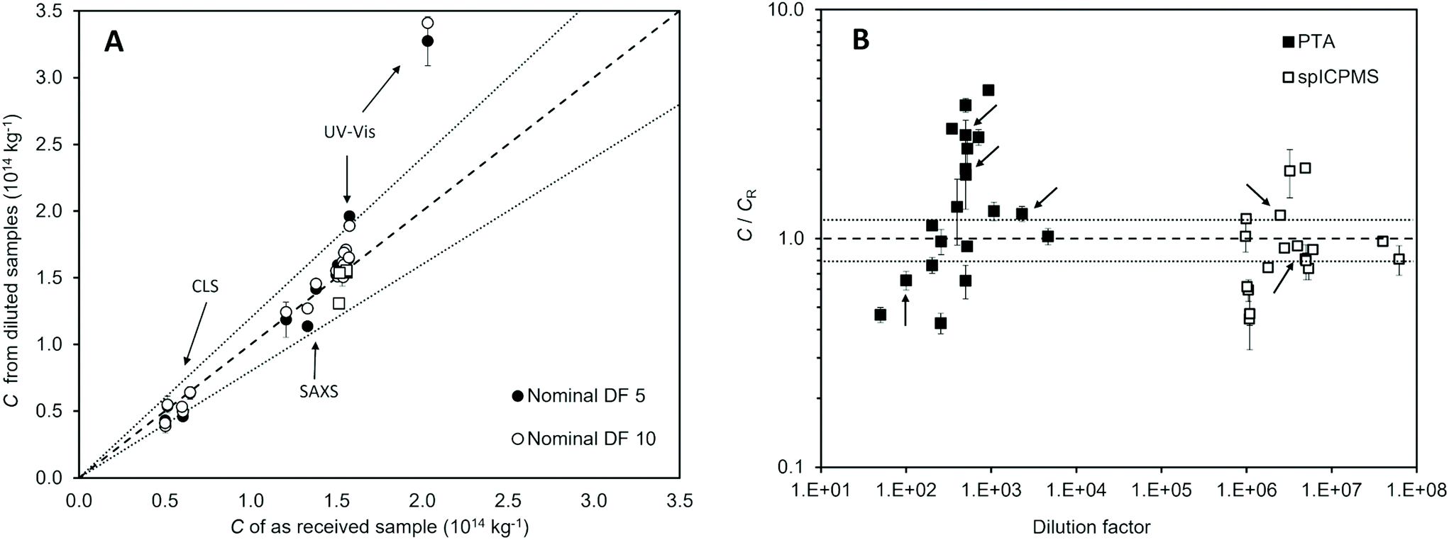 | ||
| Fig. 3 (A) Population-averaging methods: raw number concentration C of test materials from measurements of the samples diluted 5 (black marker) and 10 (white marker) times as a function of the number concentration of the undiluted sample as measured by the same laboratory using the same method. Circles relate to dilutions performed gravimetrically and squares to those performed volumetrically. (B) Particle-counting methods: raw number concentration C from measurements of the diluted aliquots relative to the accepted reference value for the test materials concentration CR as a function of the dilution factor. The arrows indicate the results from samples diluted volumetrically. In both figures, the dashed line is the identity relationship and the dotted lines show a deviation of 20%. | ||
For the UV-Vis method, the average repeatability standard deviation changed from below 0.5% to 0.6% and 1.2% for samples prepared with a dilution factor of 5 and 10 respectively. This result may reflect the analytical precision which depends upon signal intensity. In terms of measurement reproducibility, the between-labs variability changed from 1.4% to about 6% irrespective of the dilution factor. Here, we see the impact of the dilution step in the overall reproducibility of the measurement. A similar trend was observed for the CLS method. The average measurement repeatability in fact slightly improved, the standard deviations varying from 5% to 4%, possibly indicating that the diluted samples had a more optimal concentration for the instrument. However, measurement reproducibility across the laboratories worsened, with between-labs variability changing from 11% to 16% and 19% for the measurements performed on the samples diluted a factor 5 and 10 respectively.
The laboratories that participated with particle-counting methods were asked to optimise the concentration of the sample according to the laboratory best practice. The chosen concentration varied across two orders of magnitude for both methods, with no significant resulting trend on measurement bias. For those laboratories that reported a measurement result deviating more than 20% from the accepted reference value of the number concentration of the test material, the dilution factor did not appear to correlate with the bias. We note, however, that for the lower dilution factors, PTA measurement results had negative bias. This effect is attributed to overlapping of particle signals during imaging.
Discussion
Fig. 4 summarises the results of this interlaboratory study in terms of method comparability and reproducibility. The results highlighted clear distinctions between population-averaging and particle-counting methods. | ||
| Fig. 4 Results of the number concentration C of the test material as measured by the 5 methods investigated in the VAMAS TWA 34 project 10 interlaboratory study relative to the accepted reference value CR. Error bars show method between-labs variability (reproducibility standard deviation). The grey box shows the 95% confidence interval of the assigned reference value for the number concentration of the test material. | ||
A first distinction is that the population-averaging methods show better agreement between laboratories than the particle-counting methods. For example, the reproducibility of the UV-Vis method is noteworthy, with results across 24 instruments in agreement within 1.4%. This is notwithstanding instruments being from 12 different manufacturers and utilising both single and dual beam configurations, and experimental set-ups differing from each other, for example in the type of sample cuvette that was used to hold the sample. This outcome is likely to arise from the robustness of the method and the minimal sample preparation required for the measurements. The robustness reflects the maturity of the technology underpinning the method, combined with the relatively straightforward protocol, which could be reduced to two light transmission measurements (the blank and the sample) at one single wavelength (i.e. 450 nm). CLS, instead, relies on a more complex technology and requires calibration. Nonetheless, a RDS value of 11% across seven laboratories was achieved. This consistency may, in part, be due to all the instruments in the study being made by the same manufacturer. SAXS, as a population-averaging method, was performed with a lab-based and a synchrotron-based experimental set-up. The evaluated values of the mean number concentration of both set-ups only differ by 3%. This can be considered a very promising result, considering that both laboratories applied 2 different algorithms to analyse the scattering data. Similarly to UV-vis, this can be attributed to the simple sample preparation and maturity of the technique.
In contrast, the measurement reproducibility of particle-counting methods was significantly poorer across laboratories showing RSD values of 46% and 68% for the spICP-MS and PTA method respectively, despite average repeatability within each laboratory being below 12% RSD for both methods. We could not identify a trend between instrument models and measurement results and concluded that the variability is more likely due to differences between individual instruments, procedures and data processing across the laboratories. Some laboratories described at length the experimental protocol utilised to minimise potential sources of measurement uncertainty. For example, in the case of spICP-MS, some laboratories detailed how the transport efficiency was determined, the cut off value for distinguishing the nanoparticle from the continuous analyte signals identified and the background correction applied, but these practices did not appear to be in place in all laboratories. This is expected given the diverse background of the participating laboratories: while national measurement institutes may be experts in the application and standardisation of the methods, other laboratories may be using them as an internal QC and therefore be mainly concerned with method repeatability. We note that both PTA and spICP-MS may require the setting of thresholds for the discrimination of particles from background signal, depending on the instrument model. It is likely then that the need for manual setting of signal thresholds is correlated to an increase in overall measurement variability across laboratories. This may be enhanced by differences in data processing via manufacturers’ and ‘in house’ applications. There is a clear need for guidance and automation in this area, as well as transparency and standardisation in data processing.
A second distinction is that particle-counting methods require the samples to be significantly diluted in comparison to population-averaging methods. As observed from the results of the diluted samples measured by UV-Vis and CLS, the dilution step increases measurement variability across laboratories. For example, in the case of UV-Vis, measurement reproducibility worsened, with between-laboratory variability increasing from 1.4% for undiluted samples to 6% for samples following a 10-fold dilution. For PTA and spICP-MS, samples require dilutions of a factor 500 and over 1 million respectively. Most laboratories used the filtered 1 mM citrated buffer recommended for the study to minimise sample instabilities. However, the time interval between the sample dilution and its measurement was not recorded and it is therefore impossible to evaluate whether sample instabilities potentially occurring at high sample dilutions had an impact on the measurement results. Such large dilutions also raise concerns about adequate mixing and, therefore, representative sampling of the diluted material. It would be interesting to compare measurement variability for samples requiring dilution and others provided at the optimal concentration for measurements. However, we note that this is difficult to implement as operating concentrations varied significantly across laboratories, as shown in Fig. 3B. This emphasises the need for robust practice for dilutions, as an important aspect of sample preparation.
A third and final distinction is that particle-counting methods show potential for being intrinsically more accurate than population-averaging methods when sources of variability are minimised and practice is improved. One issue with the population-averaging methods is that the number concentration of the particles is the result of a theoretical model applied to the system. Here, typically, a number of other parameters of the experimental set-up or the measured sample need to be either known or determined through calibration of a known test sample. Examples of these parameters include the density and viscosity of the fluid through which the particles sediment for the CLS method. Even more critical is the reliance on the theoretical model on the properties of the measured samples. Furthermore, particles are often modelled as perfect spheres whose optical properties are inferred from literature with some knowledge of the materials they are made of. For example, in the case of UV-Vis, during the preparation of the study the extinction coefficient of the particles was calculated with an empirical method based on Mie and T-Matrix theory11 and validated by other methods.6 This approach is currently only applicable to spherical gold particles. In general, particle number concentration measurement results should include a minimum ≈20% relative error based upon uncertainty in materials’ refractive index. However, particles are rarely spherical and something as common as the presence of a coating may alter their optical properties. This argument is even stronger for heterogeneous samples, for example containing polydisperse or diverse particle populations. The particle-counting methods would still hold the potential for accurate measurements, while the population-averaging methods would require substantial modelling to interpret the results. Where measurement accuracy in number concentration is required and particle-counting methods cannot be utilised, there is a need to advance methods for the measurement of other particle attributes, primarily the optical properties such as the complex refractive index.
As far as CLS is concerned, the lack of full knowledge of the experimental parameters that enter the underpinning model, such as the optical properties of the particles and the fluid, does not fully explain the bias in the measurement results. It is likely that particle losses within the system, for example at the injection port or by absorption onto the disc and syringe walls, also contribute to this bias. In a similar fashion to spICP-MS, the CLS method could be improved by performing a calibration of the transport efficiency. A number of factors would require evaluation for the design and selection of particle calibrants suitable for specific applications, including their bulk and surface chemistry. Particle reference materials with information on their mass concentration, and more recently on their number concentration, appear useful to this purpose. It is envisaged that implementing a calibration of the “transport efficiency” within the CLS measurement protocol could result in this method being both precise and more accurate.
More information on the performance of methods for the measurement of particle number concentration will be available through the pilot study P194 of the Consultative Committee for Amount of Substance: Metrology in Chemistry and Biology (CCQM) of the International Bureau of Weights and measurements (BIPM) that was led by LGC and ran in parallel with this VAMAS study. P194 consisted of an interlaboratory comparison among the international community of national measurement institutes of the measurement of colloidal number concentration of the same batch of particles utilised for the VAMAS study. While the final outcome of the P194 pilot study has not been formally announced, preliminary results indicated that the accepted reference value for the number concentration of the test sample used in this VAMAS study is within 3.5% of the number concentration measurement resulting from the pilot study.
Overall, this study indicates that the choice of the method to adopt for the measurement of the number concentration of colloidal particles primarily depends on the field of application. If the measurements are part of a QC/QA framework, precision is probably the driving criterion for the choice. However, where accuracy is required, the choice may be different. There are certainly other types of considerations to take into account: not all methods are suitable for all materials or particle size ranges; materials may become unstable upon dilution, in which case methods requiring minimal sample preparation are preferred; samples may be expensive and limited in volume, in which case methods requiring high dilutions may be the only viable approach; samples may be susceptible to agglomeration, in which case methods with high size resolution are preferred.4 Furthermore, environmentally relevant samples contain nanoparticles in a concentration range from 10−3 g kg−1 to 10−6 g kg−1, meaning PTA and spICP-MS may be suitable for measuring them, but not UV-Vis nor CLS. In this respect, it is important for the community to have a range of methods of choice available. Studies like the current one are then important to evaluate method comparability and provide a means to validate different measurement approaches. This is particularly important for regulatory purposes. For the laboratories that took part in the study, this project also provided a means to benchmark their measurement capability. Furthermore, through this study some laboratories were able to identify problems with their equipment or update their operating procedure. The study was also useful to inform the community of the availability of the QC material LGCQC5050, the first of its kind (i.e. with an assigned value for the number concentration of the particles) and whose use will improve measurement confidence and outcome. For instrument manufacturers, the study provided an independent benchmarking and validation of their instrument models for the measurement of nanoparticle number concentration. Furthermore, the study highlighted areas for potential improvement of measurement outcome such as, for example, automation in sample handling and signal processing and improved calibration routines. The trust that the community have in such capabilities has grown as a result of this study and the knowledge developed through the preparation, delivery and outcome of the study are currently informing the development of new documentary standards and reference materials.
There is a need to extend these types of studies to a broader selection of particles that mimic more closely the attributes of real nanoparticle-based products. For example, the nanoparticle user community would benefit from the evaluation of current measurement technology for the measurement of the number concentration of (i) nanoparticles below 10 nm, which is a size range close or below the limit of detection of many liquid-based methods, but relevant for products ranging from quantum dots to viral vectors; (ii) polydisperse particle samples, with size distributions that are closer to real manufactured particle products; (iii) particles with refractive index close to that of water, for example of biological nature, with poor light scattering properties and low mass; (iv) multimodal samples, among which samples that contain populations with average sizes both in the nanometre and the micrometre size range present significant technical challenges; (v) non-spherical particles.
Conclusions
This interlaboratory study of the measurement of number concentration of colloidal nanoparticles carried out as project 10 of VAMAS TWA 34 provided the stakeholder community with important quantitative information for the comparative evaluation and validation of available measurement methods. Broadly, particle-counting methods were found to be potentially less biased than the population-averaging methods, but the latter had superior reproducibility. We discussed some of the underpinning motivations for this distinction. Importantly, we highlighted the impact on measurement outcome of experimental practice in both sample preparation and measurement execution. Despite the nanoparticles used in this study being to some extent an ideal sample, it is significant that they are currently commercially available to the user community for comparative testing. This study thus provides a substantial dataset to build confidence in the methods available for the measurement of the number concentration of colloidal samples and contributes to optimise laboratory practice and inform new documentary standards.Author contributions
CM contributed to conceptualization, data curation, formal analysis, funding acquisition, investigation, methodology, project administration, resources, supervision, validation, visualization, writing the original draft, review and editing the manuscript. MW contributed to data curation, investigation, methodology, resources and validation. DB, SCN and HGI contributed to data curation, formal analysis, investigation, methodology, resources, validation, writing the original draft, review and editing the manuscript. JD, CG and MK, KEM, MEJ and ARMB contributed to data curation, formal analysis, investigation, methodology, validation, writing the original draft, review and editing the manuscript. AGS contributed to conceptualization, formal analysis, funding acquisition, methodology, supervision, writing the original draft, review and editing the manuscript. All other authors contributed to investigation, validation and review and editing the manuscript.Conflicts of interest
There are no conflicts to declare.Acknowledgements
This work was partially funded by the 14IND12 Innanopart and 18SIP01 ISOCONCur projects of the European Union through the European Metrology Programme for Innovation and Research (EMPIR). EMPIR is jointly funded by the EMPIR participating countries within EURAMET and the European Union. The work was also funded by the UK Department of Business, Energy and Industrial Strategy through the National Measurement System programme (projects NMS/ST18-21). NILU acknowledge funding from the EU H2020 project Nanoreg2 (Grant agreement No. 646221). The University of Birmingham acknowledge funding from the EU H2020 project ACEnano (Grant agreement No. 720952). The authors thank all the people that have been involved in the delivery of this large interlaboratory study and may not be included in the list of authors.Notes and references
- F. Caputo, R. Vogel, J. Savage, G. Vella, A. Law, G. Della Camera, G. Hannon, B. Peacock, D. Mehn, J. Ponti, O. Geiss, D. Aubert, A. Prina-Mello and L. Calzolai, J. Colloid Interface Sci., 2021, 588, 401–417 CrossRef CAS PubMed.
- O. Geiss, I. Bianchi, C. Senaldi, G. Bucher, E. Verleysen, N. Waegeneers, F. Brassinne, J. Mast, K. Loeschner, J. Vidmar, F. Aureli, F. Cubadda, A. Raggi, F. Iacoponi, R. Peters, A. Undas, A. Müller, A.-K. Meinhardt, E. Walz, V. Gräf and J. Barrero-Moreno, Food Control, 2021, 120, 107550 CrossRef CAS PubMed.
- S. Weigel, R. Peters, K. Loeschner, R. Grombe and T. P. J. Linsinger, Anal. Bioanal. Chem., 2017, 409, 4839–4848 CrossRef CAS PubMed.
- C. Minelli, D. Bartczak, R. Peters, J. Rissler, A. Undas, A. Sikora, E. Sjöström, H. Goenaga-Infante and A. G. Shard, Langmuir, 2019, 35, 4927–4935 CrossRef CAS PubMed.
- J. Austin, C. Minelli, D. Hamilton, M. Wywijas and H. J. Jones, J. Nanopart. Res., 2020, 22, 108 CrossRef CAS.
- A. Schavkan, C. Gollwitzer, R. Garcia-Diez, M. Krumrey, C. Minelli, D. Bartczak, S. Cuello-Nuñez, H. Goenaga-Infante, J. Rissler, E. Sjöström, G. B. Baur, K. Vasilatou and A. G. Shard, Nanomaterials, 2019, 9, 502 CrossRef CAS PubMed.
- A. R. Montoro Bustos, E. J. Petersen, A. Possolo and M. R. Winchester, Anal. Chem., 2015, 87, 8809–8817 CrossRef CAS PubMed.
- T. P. J. Linsinger, R. Peters and S. Weigel, Anal. Bioanal. Chem., 2014, 406, 3835–3843 CrossRef CAS PubMed.
- E. J. Petersen, A. R. Montoro Bustos, B. Toman, M. E. Johnson, M. Ellefson, G. C. Caceres, A. L. Neuer, Q. Chan, J. W. Kemling, B. Mader, K. Murphy and M. Roesslein, Environ. Sci.: Nano, 2019, 6, 2876–2896 RSC.
- A. G. Shard, K. Sparnacci, A. Sikora, L. Wright, D. Bartczak, H. Goenaga-Infante and C. Minelli, Anal. Methods, 2018, 10, 2647–2657 RSC.
- A. G. Shard, L. Wright and C. Minelli, Biointerphases, 2018, 13, 061002 CrossRef CAS PubMed.
- S. Cuello-Nuñez, I. Abad-Álvaro, D. Bartczak, M. E. del Castillo Busto, D. A. Ramsay, F. Pellegrino and H. Goenaga-Infante, J. Anal. At. Spectrom., 2020, 35, 1832–1839 RSC.
- ISO, 17867:2020 Particle size analysis—Small angle X-ray scattering (SAXS), 2020 Search PubMed.
- ISO, TR 22814:2020 Good practice for dynamic light scattering (DLS) measurements, 2020 Search PubMed.
- ISO, 22412:2017 Particle size analysis—Dynamic light scattering (DLS), 2017 Search PubMed.
- ISO, 13318-2:2007 Determination of particle size distribution by centrifugal liquid sedimentation methods—Part 2: Photocentrifuge method, 2007 Search PubMed.
- ISO, 13318-1:2001 Determination of particle size distribution by centrifugal liquid sedimentation methods—Part 1: General principles and guidelines, 2001 Search PubMed.
- ISO, TS 19590:2017 Nanotechnologies—Size distribution and concentration of inorganic nanoparticles in aqueous media via single particle inductively coupled plasma mass spectrometry, 2017 Search PubMed.
- ISO, 19430:2016 Particle size analysis—Particle tracking analysis (PTA) method, 2016 Search PubMed.
- ISO, 27891:2015 Aerosol particle number concentration—Calibration of condensation particle counters, 2015 Search PubMed.
- ISO, WD 13319-2 Determination of particle size distribution—Electrical sensing zone method—Part 2: Tuneable resistive pulse sensing method, In development, 2023 Search PubMed.
- ISO, TR 24672 Nanotechnologies - Guidance on the measurement of nanoparticle number concentration, In development, 2022 Search PubMed.
- LGCQC5050 Colloidal gold nanoparticles, https://us.lgcstandards.com/US/en/Colloidal-gold-nanoparticles/p/LGCQC5050, 2021.
- C. Minelli, M. Wywijas, D. Bartczak, S. Cuello-Nuñez and H. Goenaga-Infante, NPL report, 2018, AS 98.
- W. Haiss, N. T. K. Thanh, J. Aveyard and D. G. Fernig, Anal. Chem., 2007, 79, 4215–4221 CrossRef CAS PubMed.
- A. J. Allen, F. Zhang, R. J. Kline, W. F. Guthrie and J. Ilavsky, J. Appl. Crystallogr., 2017, 50, 462–474 CrossRef CAS PubMed.
- B. L. Henke, E. M. Gullikson and J. C. Davis, At. Data Nucl. Data Tables, 1993, 54, 181–342 CrossRef CAS.
- C. T. Chantler, J. Phys. Chem. Ref. Data, 2000, 29, 597–1056 CrossRef CAS.
- B. R. Pauw, C. Kästner and A. F. Thünemann, J. Appl. Crystallogr., 2017, 50, 1280–1288 CrossRef CAS PubMed.
- A. Braun, V. Kestens, K. Franks, G. Roebben, A. Lamberty and T. P. J. Linsinger, J. Nanopart. Res., 2012, 14, 1021 CrossRef.
- W. Wohlleben, V. A. Coleman and D. Gilliland, in Characterization of Nanoparticles, ed. V.-D. Hodoroaba, W. E. S. Unger and A. G. Shard, Elsevier, 2020, pp. 225–247, DOI:10.1016/B978-0-12-814182-3.00015-8.
- F. Laborda, J. Jiménez-Lamana, E. Bolea and J. R. Castillo, J. Anal. At. Spectrom., 2013, 28, 1220–1232 RSC.
- A. Hineman and C. Stephan, J. Anal. At. Spectrom., 2014, 29, 1252–1257 RSC.
- H. E. Pace, N. J. Rogers, C. Jarolimek, V. A. Coleman, C. P. Higgins and J. F. Ranville, Anal. Chem., 2011, 83, 9361–9369 CrossRef CAS PubMed.
- M. D. Montaño, J. W. Olesik, A. G. Barber, K. Challis and J. F. Ranville, Anal. Bioanal. Chem., 2016, 408, 5053–5074 CrossRef PubMed.
- F. Benvenuto, H. Haddar and B. Lantz, SIAM J. Appl. Math., 2016, 76, 276–292 CrossRef.
- Xenocs SAS, XSACT software: X-ray Scattering Analysis and Calculation Tool, https://www.xenocs.com/saxs-products/xsact-software/, (accessed 7th May 2021).
- C. M. Maguire, K. Sillence, M. Roesslein, C. Hannell, G. Suarez, J.-J. Sauvain, S. Capracotta, S. Contal, S. Cambier, N. El Yamani, M. Dusinska, A. Dybowska, A. Vennemann, L. Cooke, A. Haase, A. Luch, M. Wiemann, A. Gutleb, R. Korenstein, M. Riediker, P. Wick, P. Hole and A. Prina-Mello, J. Micro Nano-Manuf., 2017, 5(4), 041002–041012 CrossRef.
- K. Murphy, J. Liu, A. R. Montoro Bustos, M. E. Johnson and M. R. Winchester, NIST Special Publication 1200-21, 2015 Search PubMed.
- J. Liu, K. E. Murphy, R. I. MacCuspie and M. R. Winchester, Anal. Chem., 2014, 86, 3405–3414 CrossRef CAS PubMed.
- I. Strenge and C. Engelhard, J. Anal. At. Spectrom., 2016, 31, 135–144 RSC.
Footnotes |
| † Electronic supplementary information (ESI) available. See DOI: 10.1039/d1nr07775a |
| ‡ Current address: ET Enterprises Ltd, 45 Riverside Way, Uxbridge UB8 2YF, UK. |
| § Current address: University of Siegen, Adolf-Reichwein-Str. 2, D-57076 Siegen, Germany. |
| ¶ Current address: TOFWERK AG, Schorentrasse 39, 3645 Thun. |
| || Current address: Calibration and Service, Topas GmbH, Gasanstaltstraße 47, 01237 Dresden, Germany. |
| ** Current address: Great Ormond Street Institute of Child Health, University College London, London, UK. |
| †† Current address: CNRS, Université de Lyon, Bât Brillouin Domaine Scientifique Doua, 69622 Villeurbanne CEDEX, France. |
| ‡‡ Current address: Particular Sciences Ltd, Rosemount Business Park, Ballycoolin, Dublin 11, Ireland. |
| §§ Current address: Department of Materials, Department of Bioengineering and Institute of Biomedical Engineering, Imperial College London, London, SW7 2AZ, UK. |
| ¶¶ Current address: Innovation in Research and Engineering Solutions, Rue Koningin Astridlaan 59B, 1780, Wemmel, Belgium. |
| This journal is © The Royal Society of Chemistry 2022 |