Self-assembled cellulose nanofiber–carbon nanotube nanocomposite films with anisotropic conductivity

Abstract

In this study, a nanocellulose-based material showing anisotopic conductivity is introduced. The material has up to 1000 times higher conductivity along the dry-line boundary direction than along the radial direction. In addition to the material itself, the method to produce the material is novel and is based on the alignment of cationic cellulose nanofibers (c-CNFs) along the dry-line boundary of an evaporating droplet composed of c-CNFs in two forms and conductive multi-walled carbon nanotubes (MWCNTs). On the one hand, c-CNFs are used as a dispersant of MWCNTs, and on the other hand they are used as an additional suspension element to create the desired anisotropy. When the suspended c-CNF is left out, and the nanocomposite film is manufactured using the high energy sonicated c-CNF/MWCNT dispersion only, conductive anisotropy is not present but evenly conducting nanocomposite films are obtained. Therefore, we suggest that suspending additional c-CNFs in the c-CNF/MWCNT dispersion results in nanocomposite films with anisotropic conductivity. This is a new way to obtain nanocomposite films with substantial anisotropic conductivity.

---

Introduction

There is an increasing demand for thinner, cheaper, lighter, and more eco-friendly electrically conductive films and composites¹ with anisotropic properties^2,3 for applications including optics, sensors, actuators, aerogels, mechanical reinforcement of advanced materials, and growth guiding substrates including hydrogels for biomedical applications.^2,3 There are various motivations for material alignment in these applications, such as a need for anisotropic properties in adjusting the stiffness and strength of structural materials; optimizing the reinforcement efficiency in fiber-reinforced composites; and mimicking the topography and architecture of native tissues in biomedical materials and applications, especially related to cell alignment in vitro.² The assembled oriented particles with a high aspect ratio generally exhibit anisotropic physical properties. If the particle is also conductive, an anisotropic conductivity may result, which is potentially useful in electronic components, capacitors, sensors, electromechanical actuators, etc. In the assembled structures of high aspect ratio nanomaterials, the differences in the electric current parallel and perpendicular to the orientation results in conductivity anisotropy.⁴

Cellulose nanofibers (CNFs) are an excellent candidate as a primary ingredient in such composites since they provide an eco-friendly and low-cost material alternative¹ with the potential to align and offer anisotropic properties for the resulting composite material.² CNF-based electrically conducting materials have been produced by coating, blending or doping CNFs with conductive nanoparticles such as carbon nanotubes (CNTs). CNFs act as a matrix and dispersant of the conductive CNT component.^5–7 These nanomaterials together provide a combination of their superior properties such as the film forming potential,⁸ favourable mechanical and chemical properties, colloidal stability, cytocompatibility^9–15 and biocompatibility of CNFs,^9–11 and high mechanical strength, stiffness, and electrical and thermal conductivity of CNTs.¹⁶

Chemically added charged groups influence the physicochemical properties of CNFs¹⁷ and can improve their processability and performance.¹⁸ Treatment with cations can be performed to render cellulose nanofibers cationic by introducing positive charges on their backbone. Cationic CNFs (c-CNFs) can be used in both high-end applications as nanocomposites and high volume applications,¹⁹ and are gaining increasing attention as a potential novel nanomaterial with tailored properties in more specialized applications.^20,21 Cationic CNFs have the capability to align along the evaporating droplet boundary line by self-assembly mechanisms.²² By dispersing carbon nanotubes with c-CNF, there is potential to form aligned structures also in electrically conductive composites. None of the previous studies have used c-CNFs in the dispersion of CNTs. In the current study, the use of cationic CNFs as a dispersing and stabilization agent is reported for the first time and their alignment is studied in nanocomposite films.

Superior CNF properties are often challenging to transfer into optimal macroscale performance. In plants, CNFs are naturally aligned into highly hierarchical structures. However, despite several attempts and extensive research, the realignment of disintegrated and fibrillated CNFs remains challenging.² While the alignment of CNFs alone is challenging as such, it is extremely challenging to align CNFs in composites.² Another challenge is dispersing CNTs because of their self-aggregation tendency especially in aqueous media,²³ which on the other hand is often a prerequisite for hydrophilic CNFs.²⁴ While CNT blending in aqueous media is poor due to strong self-aggregation, sonication treatments have been introduced to obtain homogeneous dispersions.^6,25

Several research groups have reported the ability of CNFs to disperse CNTs in aqueous media using sonication and act as a stabilization agent in the CNF–CNT dispersion; furthermore, a stable dispersion can be obtained without the use of surfactants, which have been commonly used.^7,26–28 Chemical modifications of at least one of the nanomaterial components by the introduction of charged groups may enhance the dispersing effect. In addition, repulsive forces may prevent the re-agglomeration of the particles in the dispersion state resulting in a more stable dispersion.¹ It has been shown, e.g., that anionic CNFs enhance the dispersion of CNTs.²⁹

Sonication is one of the methods used for attaining the dispersion of nanoparticles in aqueous media. It is based on inertial cavitation where imploding cavities, which are known to exist at the boundaries of materials, generate intensive streams of molecules.³⁰ In sonication, a high energy density is introduced to the CNT–CNT interface, which is high enough to cause initial separation of the nanotubes by breaking non-covalent forces between tubes. However, the used amount of energy should be optimized such that only non-covalent forces are overcome and the carbon nanotube backbone remains intact. An overly high sonication energy can cause carbon bond breakage inside individual nanotubes, which deteriorates their ballistically conducting nature. The dispersion quality and functionalization obtained in sonication depend on the used sonication energy, medium, surfactant type, and surfactant amount.^6,25,31

In this study, we present a method to produce self-assembled nanocomposite films with adjustable anisotropic thermal and electrical conductivity. The method uses sonochemical treatment and c-CNFs to disperse multiwall carbon nanotubes (MWCNTs). The resulting dispersion is assembled with the help of additional, suspended c-CNFs, which are based on the previously reported c-CNF alignment along an evaporating boundary line.²² We also show how the alteration of the composition and pre-treatment of the two nanomaterials enable the fabrication of nanocomposite films with either isotropic or anisotropic properties. Controlled nanomaterial assembly commonly requires more time, high energy consumption, and expensive proprietary technology.³² The method described in this article is simple, quick, efficient, and safe compared to current attempts to control the assembly of nanomaterials. Such novel nanocomposites could be used as a cell guidance material with cells that benefit from the mechanical improvements offered by MWCNTs or in applications in which anisotropic heat or current conductivity is essential. CNF-based electrically conductive composites have many advantages although many challenges remain, e.g. related to electrical connectivity. In our previous study, we have also shown that MWCNTs can be effectively dispersed with unmodified CNFs with the help of surfactants and form highly conductive nanocomposite films with a relatively low MWCNT concentration.⁶ In the present article, we combine the advantages of these observed phenomena to create a totally new methodological concept: c-CNFs are used as an aid to disperse MWCNTs homogeneously to form a stable dispersion, and additional c-CNFs in the dispersion undergo interfacial self-assembly with the high energy sonicated (hes-) hes-c-CNF/MWCNT dispersion, resulting in a novel nanocomposite film with anisotropic properties.

Results and discussion

Theoretical assumption and modelling

In our previous study, we showed c-CNF alignment along an evaporating boundary line. In the present study, we studied if a conducting component (MWCNT) can be added, and still obtain anisotropic film properties. We also have studied dispersing MWCNTs using CNFs and sonication, and thus hypothesize that CNFs used as a dispersant form a stronger complex with MWCNTs, compared to CNFs that are added to the system by more gentle manual mixing. Based on our previous findings, we hypothesize as shown in Fig. 1, that an isotropic conductive film is obtained when water from the hes-c-CNF/MWCNT dispersion is evaporated and an anisotropic film is obtained when water is evaporated from a suspension composed of the hes-c-CNF/MWCNT dispersion and additional c-CNFs. Fig. 1 conceptually depicts the hypothesis for explaining the structural composition and the electrical conductivity of the films fabricated from a dispersion (control) or with suspended free c-CNFs. Sonochemical treatment of c-CNFs and MWCNTs is hypothesized to result in a stable dispersion. Nanocomposite films formed from this hes-c-CNF/MWCNT dispersion (control samples) are uniformly conducting in all directions (that is, isotropic films), as illustrated by the left-side schematic in Fig. 1(a and b). When free c-CNFs are added to the stable dispersion, a self-assembled structure is formed during evaporation, providing anisotropic electrical properties (that is, assembled films), as depicted in the right-hand-side schematic in Fig. 1(b and c). Fig. 1 shows simulations of electrical properties of isotropic control (a) and anisotropic assembled (d) nanocomposite films using the finite element method (FEM) using COMSOL Multiphysics® Version 5.4 (COMSOL, Inc. USA). Fig. 1e and g show a hypothesized structure at the nanoscale, highlighting the aligning component, which is suspended c-CNFs (Fig. 1g) in the assembled films, while the repeating, alternating structure in Fig. 1g is an oversimplification. The structure is believed to alter at the nanoscale, and the boundaries between aligning c-CNFs and more entangled hes-c-CNF/MWCNTs are not as clear as shown in Fig. 1g. We assume the increasing amount of c-CNFs between the “layers” from the edge towards the center (based on the resistance results presented in Fig. 3). A film manufactured from the hes-c-CNF dispersion exhibits even conduction. The high energy sonication treatment causes c-CNF fibrillation and chopping, resulting in smaller hes-c-CNFs (Fig. 1f) compared to the suspended c-CNFs that have not been high energy sonicated (Fig. 1g). Using thermal imaging and resistance measurement, we aim to confirm this presented Hypothesis of the assembled film with anisotropic conductivity. Furthermore, we performed micro- and nanostructural characterization to provide support for the Hypothesis of an assembled structure and the dispersal effect of c-CNFs. While the exact structure and alignment are challenging to show at the nanoscale, in the next sections we present a variety of results supporting the hypothesis in which the c-CNF alignment drives the formation of anisotropically conductive films.

Fig. 1 Conceptual images of the hypothesized structure of nanocomposite films (b, c, e, f, and g). Left side (b and e) represents the control film manufactured using the hes-c-CNF/MWCNT dispersion. Right side of (c and g) represents the assembled nanocomposite film manufactured using the c-CNF + hes-c-CNF/MWCNT suspension. The schematic represents simulations of electrical properties of an isotropic control (a) and anisotropic self-assembled (d) nanocomposite films using finite element method (FEM). Alignment direction of free assembling c-CNFs is shown in g. Light grey represents c-CNFs, while dark grey is MWCNTs. In the control film (e) dark grey MWCNTs are surrounded by the c-CNF matrix (white surroundings). During dispersion preparation, i.e. sonication, c-CNFs are fibrillated and degraded in length such that they cover the MWCNT surface (f). The added c-CNFs during suspension preparation are larger in size compared to hes-c-CNF. The repeating, alternating structure in (g) is an oversimplification. The illustrations are oversimplified and not in scale and do not try to show the actual sizes or actual structure of the assembled film but give an overview of the hypothesized repeating structure at the nanoscale, and show the difference between control and assembled films.

Anisotropy characterization: electrical conductivity of nanocomposite films using heat maps

The heat map results confirm that evaporation of the aqueous medium from the dispersion results in uniform electrically conductive nanocomposite films, while that evaporated from the suspension (S1–S3) formed self-assembled nanocomposite films with anisotropic electrical conductivity. An overview of the differences in conductivity between the isotropic control film and the self-assembled anisotropic films is visible in IR heat maps (Fig. 2). The control film obtained from the sonicated stable homogeneous hes-c-CNF-MWCNT dispersion shows an even temperature across the film when a constant voltage is applied on the film surface through the silver ink contacts, suggesting that the current follows the shortest route, as shown in the IR-image captured soon after the beginning of heating (Fig. 2a), before heat has spread evenly across the film. Current flows through the centre of the film, as hypothesized for uniformly conducting films. The result is consistent with the results obtained with the finite element model illustrated in Fig. 1a. Interestingly, when a solution containing additional free c-CNFs is suspended with the sonicated hes-c-CNF-MWCNT dispersion and the aqueous medium is evaporated, the resulting film possesses heat zones (Fig. 2b) instead of homogeneous temperature distribution as in the control film (the fully heated control film is not shown here). In the infrared images shown in Fig. 2b, higher temperatures indicate the paths that the current passes through. In the self-assembled films, the centre area shows a lower temperature, indicating that the current is restricted to pass through the centre line, which is the shortest path from terminal to terminal.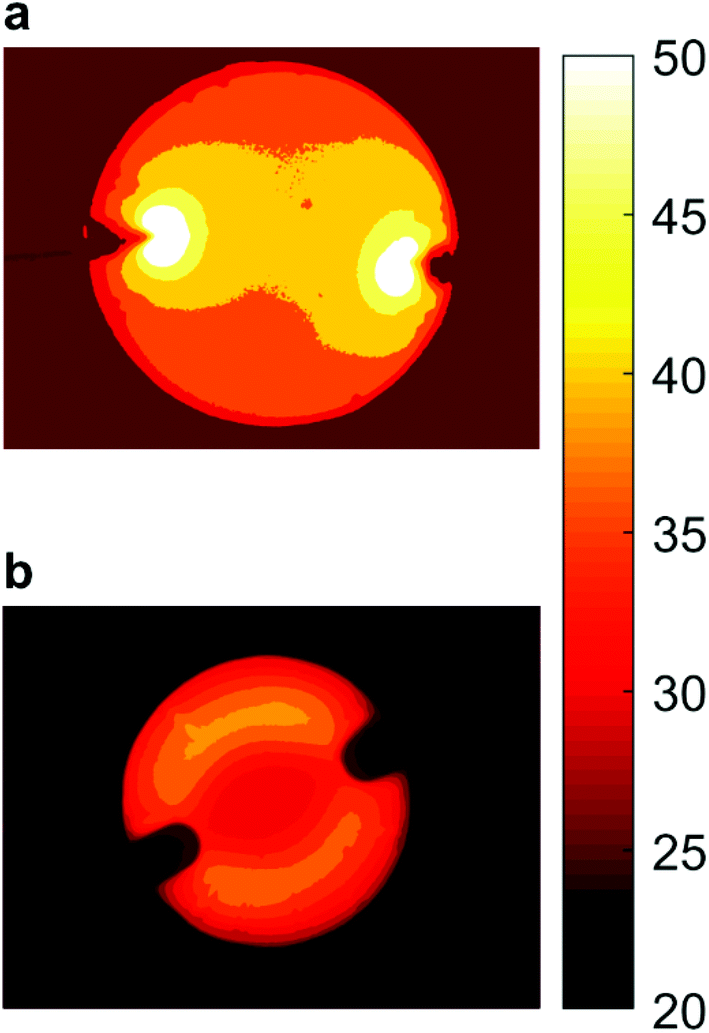

Fig. 2 Difference in thermal conductivity between control and assembled films. IR-imaging of the isotropic control nanocomposite film (a) and self-assembled anisotropic nanocomposite film S1 (b) when a current is applied to the structure so that heating phenomenon occurs.

Anisotropy characterization: electrical conductivity analysis using resistance measurement

The IR-imaging depicts the anisotropic electrical properties of the self-assembled films at the macroscopic scale. Resistances determined (Fig. 3 and Fig. S1 of ESI†) using the measurement protocol (Fig. 8) confirm the findings obtained with the IR-imaging: the control film shows isotropic behavior, while self-assembled films S1–S3 are electrically anisotropic.

Fig. 3 Resistance of the assembled (S1–S3) and control (C) films. Resistance measurement protocol (presented at the upper row). Results for films S1–S3 and control from locations along the radial line (measurements A–C presented at the middle row) and along circles 1 and 3 (measurements D and E, at the lower row). In measurements, locations n_n–p_n, n_n and p_n stand for negative and positive probe locations, respectively.

The control films show relatively constant resistance throughout the film, as illustrated in Fig. 3. In contrast to the control films, the self-assembled films S1–S3 show evident anisotropy. The resistance increases along the centre line towards the centre (measurements A and C, Fig. 3), while along the circle it essentially remains constant, measured from both circles 1 and 3 (measurements D and E, respectively, Fig. 3).

In measurement A, the measurement probes are moved along the centre line, maintaining a constant probe distance, depicting an increase in resistance when moving towards the centre, and a subsequent decrease in resistance when moving from the centre towards the edge of the film. The resistance increase is apparent in each measurement towards the centre, although the increase is larger closer to the centre.

Measurement B demonstrates an increase in resistance along the different circular zones, that is, circles when zones are located closer to the centre. Thus, the resistance continually increases even though the probe distance decreases. A difference in the isotropic control film is evident, where the resistance decreases with reduced probe distances, as is expected for an evenly conducting film. Measurement B includes radial line locations that correspond to the location at 180° in measurement D and E, further confirming lower resistances along a circular zone than along the centre line.

In measurement C, one probe remains in location 1 in all measurements, while the other probe is moved along the centre line, that is, the probe distance increases in the subsequent measurements. Measurement C again confirms the difference between the control and assembled films. The resistance in the control film increases slightly with an increasing probe distance, while in the self-assembled films S1–S3, the resistance increases significantly until the centre, with a subsequent decrease after the centre towards the opposite edge of the film. This is in accordance with the Hypothesis, which assumes the current passes through the conducting zones, that is, along the circles in the self-assembled S1–S3 films – instead of the shortest route across the centre, as in the control films.

The resistance measured along circle 1 and along circle 3 in measurements D and E, respectively, is consistent with the Hypothesis. In the control film, the resistance in circle 1 is slightly higher than that in circle 3. This is due to the longer probe distance in circle 1 than in circle 3. Thus, the result is compatible for a uniformly conducting film. Opposite to the control film, the self-assembled films (S1–S3) have a lower resistance in circle 1 than in circle 3, even though the probe distance decreases in circle 3. The result is in accordance with measurement B (Fig. 3), which demonstrated the increase in the resistance along the different circles when zones are located closer to the centre. Opposite results between the control films and films S1–S3 further confirm the Hypothesis of an anisotropic assembly in S1–S3. The increase in resistance of all the measured films (control, S1–S3) when moving along circles 1 or 3 results from the increasing probe distance.

The demonstrated anisotropy is stronger in S2 than in S1 because of a higher concentration of suspended free c-CNFs in S2 than in S1. The concentration of suspended free c-CNFs is equal in S2 (supernatant) and S3 (supernatant sonicated 625 kJ g⁻¹). Even though the concentration of suspended c-CNFs is equal in S2 and S3, the anisotropy is stronger in S3. Suspended c-CNFs are more fibrillated in S3 compared to S2, thus the nanofibrils in S3 are expected to be smaller in diameter.

When comparing resistances on approximately the same distance along circle 1 and along the radial line, that is, probe locations (measurement D) and 1–4 (measurement C), respectively – the resistance is approximately 10-fold, 100-fold, and 1000-fold higher in the radial line compared to the resistance along circle 1 for S1, S2, and S3, respectively. Comparing the length of the radial line from the edge until the centre of the film – that is, locations 1–5 (measurement C) – and the corresponding distance on circle 1 – that is, locations (measurement D) – the difference in the resistance along the centre line (from location 1 to location 5) is even higher, approaching 100-fold and 1000-fold in S1 and S2, respectively. In S3, the resistance in the corresponding locations remains the same as between locations 1 and 4, that is, approximately 1000-fold. In all self-assembled films S1–S3, the highest resistance is found in the middle of the films and is approximately 0.5 MΩ for S1 in locations 4–5, while approaching 10 MΩ and 100 MΩ in S2 and S3, respectively. Composites were subjected to an electric field for at least 11 min as the measurements were repeated three times for each film, to demonstrate the stability of the films. In addition, three parallel films were fabricated and measured in order to show the repeatability of the film manufacture. Parallel and repeat resistance measurement results are summarized in ESI Fig. S1† and the results indicating the stability of the films in the electric field are presented in ESI Fig. S1 and S2.†

Anisotropy characterization: topographical alignment

Scanning electron microscopy images were collected at different locations on the film to perform SEM image-based orientation analysis. Cytospectre software³³ was used for the analysis to obtain the degree and direction of orientation from the assembled films or the lack of orientation from the control films. Using spectral analysis, two different values were obtained to confirm anisotropy from the SEM images of assembled films (Fig. 4). First, we use a parameter called the circular variance (CV) value to show the difference in the degree of orientation between assembled and control films. CV was determined from each image (Fig. 4a, b and h) in order to describe to degree of orientation. A CV value of 1 refers to perfect isotropy, while a value of 0 is perfect anisotropy. While the CV value of the isotropic control film is close to 1 (indicating isotropy), that of assembled films is remarkably lower (indicating more anisotropic topography compared to control films), Fig. 4h.

Fig. 4 Low vacuum SEM scans from the surface of the S3 (a) and control (b) films. Scale bar in a and b is 50 μm. Examples of scanning locations (c) and the corresponding mean orientation angles (e) of the assembled films. The mean orientation angles for the control films are not presented, as the circular variance is close to 1 in all scanning locations of the control films (d), so no primary alignment direction is expected. A graphical illustration (f) of the orientation describes the orientation direction in Scanning Point 2 (SEM image in (a)), while isotropy (g) is confirmed for the location seen in SEM image (b). Circular variances of the films S1, S2, S3 and control (h). Circular variance averages (n = 4) or the films S1, S2, S3, and control are 0.76, 0.65, 0.67 and 0.96, respectively. Perfect isotropy corresponds to circular variance value 1, while 0 stands for perfect anisotropy.

In addition to the CV value, a mean orientation angle of each image location was determined in order to show the orientation direction along the evaporating boundary line. While CV only describes the degree of orientation – that is, isotropy or anisotropy – the mean orientation can be used to show if the orientation direction is according to our hypothesis; that is, along the evaporating dry-line boundary, and thus along the imaginary circles. For this purpose, the films were scanned on a specific surface location, and the scanning location (Fig. 4c) was compared with the mean orientation angle (Fig. 4e) of the analyzed images (Fig. 4a and b as an example) and the expected orientation direction according to our hypothesis (Fig. 1). The mean orientation is presented only for assembled films, as the control films have no expected orientation according to the analyzed CV values. However, an example of the mean orientation angle for the control sample is shown in Fig. 4b for the scanning location shown in Fig. 4d.

The CV analysis (Fig. 4h) confirmed the expected higher degree of orientation of the assembled films compared to the control films, as discussed below. The degree of anisotropy is greater for assembled films than for control films with more isotropic CV values. As the film also contains isotropic MWCNT arrangement (Fig. S4a, e and i†), CV values are not expected to be close to zero. This is because only the added c-CNFs are expected to align along the dry-line boundary during evaporation. Thus, the average CV values (n = 4) of the assembled films S1, S2, and S3 are 0.65–0.76 (Fig. 4h), compared to the previously determined 0.27,²² of highly anisotropic pure c-CNF films. The average circular variance (n = 4) of the control films is 0.96.

In summary, CV values show a higher degree of anisotropy for assembled films than control films do, while the mean orientation angles in specific locations show orientation along the circle. This indicates orientation along the dry-line boundary during the evaporation of the liquid.

When analyzing the low vacuum SEM surface scans (one example in Fig. S5†), it is evident that the hes-c-CNF fibrillates during sonication, as the larger fiber bundles that can be seen in S1 and S2 (Fig. S5a and b†) are missing in S3 (Fig. S5c†), in which the suspended component was hes-c-CNF. The decreased size of hes-c-CNF compared to c-CNFs is due to the high energy sonication treatment of the former. The sonication energy used in suspended hes-c-CNF in S3 is the same as that used to prepare the hes-c-CNF/MWCNT dispersion. The degree of orientation is significantly higher in the case of S3 (manufactured using hes-c-CNF + hes-c-CNF/MWCNT) compared to the control film (manufactured using hes-c-CNF/MWCNT). This confirms that the alignment is not dependent on the suspended c-CNF size, but the addition of the suspended c-CNFs.

Nanocomposite film structure supporting the hypothesis

To confirm the basis behind the observed electric anisotropy, structural characterization of the films and their components was performed using scanning electron microscopy (SEM), (scanning) transmission electron microscopy ((S)TEM) and atomic force microscopy (AFM). According to SEM, (S)TEM, and AFM imaging, MWCNTs were in random orientation in all control and self-assembled (S1–S3) films. Thus, no alignment/orientation of MWCNTs was observed (Fig. 5c and S4a and e†). While it is challenging to observe topographical alignment from the densely packed film surface of low weight element components, SEM images were analyzed using spectral analysis in order to detect possible anisotropy and orientation direction. Spectral analysis (Fig. 4) was consistent with our hypothesis, that there is topographical anisotropy in the direction expected, i.e. parallel to the evaporating boundary line. In our previous study²² the evaporation was studied and we showed c-CNF alignment along (parallel) the evaporating boundary line (from edge towards the center). This indicates that suspended c-CNFs are the aligning component and are the driving component of the self-assembly. Surface examination of a film prepared from the hes-c-CNF/MWCNT dispersion (control, Fig. S4i†) shows well-dispersed MWCNTs and no aggregates were observed. The edges of the control film (Fig. 5b) and the assembled film S1 (Fig. 5a) were observed because we previously reported that the self-assembly of c-CNFs begins on the droplet boundary line.²² SEM characterization of the film edges (Fig. 5a and b) show that, in the control film (Fig. 5b), the edges are not as uniform as in the self-assembled films (Fig. 5a). MWCNTs can be seen on the edge of the control films, while no MWCNTs are visible in the edge of the self-assembled films.

Fig. 5 SEM edge view of the intact assembled (a) and control (b) nanocomposite film. Surface scan with visible MWCNTs is presented in (c). More SEM images are presented in ESI file Fig. S4.† Scale bar sizes are as follows: 200 nm (a and b), and 1 μm (c).

According to the Hypothesis, we expect free c-CNF alignment on the evaporating boundary line; thus, the film edge should be relatively smooth, as demonstrated in Fig. 5a. In addition, the outmost film edge is slightly thickened in the case of the self-assembled films, which is consistent with our previous observation of droplet boundary line pinning in the beginning of evaporation²² and accumulation of aligned fibers on the boundary edge. Therefore, a slight ‘coffee ring’ effect is expected in the very beginning of the evaporation, after which the evaporation progresses evenly as the nanosized fibers of the suspension align parallel to the boundary line. The droplet evaporates by shrinking towards the centre and allows more time for the assembly of c-CNFs in the beginning of droplet evaporation, that is, further from the droplet centre.²² In the previous study, we investigated the droplet evaporation of free c-CNFs in more detail, and it is known that evaporation closer to the centre is faster due to the smaller droplet volume. This likely influences the film thickness, composition, and anisotropic properties. More structural characterization is presented in ESI file Sections 1.3 and 1.4.†

The dispersive effect of the c-CNFs on MWCNTs is visible in the AFM scan of the film surface (Fig. 6a), as well as of the dilute dispersion (Fig. 6b), with no visible MWCNT aggregates present. The dilute dispersion presents larger molecules, that is, MWCNTs. Hes-c-CNF in the dispersion (Fig. 6b) is smaller than c-CNFs in the supernatant (Fig. 6c) due to a higher degree of sonication. This is observed also from surface scans (ESI Fig. S5†), which confirms the presence of larger nanocellulose fibers in S1 and S2 films fabricated using supernatant c-CNFs, while S3 was fabricated using 625 kJ g⁻¹ sonicated hes-c-CNF in which larger fibers are not detected. The TEM images show the c-CNF matrix rigidly attached to individual MWCNTs (Fig. 6d and e) on a torn film boundary. For comparison, Fig. 6f shows the TEM image of pristine multi-wall carbon nanotubes. Similar to SEM imaging, the challenge of TEM is to distinguish individual cellulose nanofibrils from a densely packed matrix. (S)TEM (secondary electron imaging) was used to distinguish individual c-CNFs on top of MWCNTs (Fig. 6h), from a torn film boundary (Fig. 6g). Untreated MWCNTs were examined using STEM (Fig. 6i) for comparison.

Fig. 6 Nanostructure comparison. AFM (a–c) and (S)TEM (secondary images) (d–i) of the film surface (a), torn film boundary ( d, e and g), dilute dispersion (b), dilute c-CNF supernatant (c), untreated MWCNTs (f and i) and individual MWCNTs with c-CNFs on the surface (h) from a torn nanocomposite film. Scale bar sizes in (a–c) is 500 nm.

Based on the findings of SEM and AFM examination, we can confirm that c-CNFs work as a dispersing/stabilizing agent for MWCNTs. The present study is the first to demonstrate the successful use of c-CNFs to disperse MWCNTs. However, further optimization for sonication energy per dry mass and materials’ concentrations should be done.

Chemistry and interactions of the components: Interactions and chemical characterization

To attain more information regarding the effects of sonication treatments and interactions between cationic nanocellulose and carbon nanotubes, magic angle spinning (MAS) NMR spectroscopy is applied. The objectives are to examine possible chemical modification and to evaluate the interaction between c-CNFs and MWCNTs. The ¹H NMR spectra in ESI Fig. S7† illustrate the hydrogen peaks of the untreated c-CNFs (Fig. S7a†) which were used as a reference for the examination of the effects of sonication treatments on the sonicated samples (Fig. S7b and c† for hes-c-CNFs, respectively, and Fig. S7d† for the hes-c-CNF-MWCNT dispersion and ESI 1.5† in more detail).

The intensity and the area of the signal peak at 2.1 ppm results from –CH₃ groups of the functionalized hydroxypropyltrimethylammonium side chain and remain relatively unchanged in c-CNF samples (Fig. S7a–c†), indicating that the functional group remains intact and relatively stable throughout the sonication treatments. Untreated c-CNFs and c-CNFs sonicated with 625 kJ g⁻¹ provide the same signals. Thus, the effect of sonication on the chemical structure of c-CNF is assumed negligible. Evaluating the interaction between c-CNFs and MWCNTs during sonication is not straightforward from ¹H NMR spectra (Fig. S7d†) as the analyte is merged and signals are broad and overlapping. However, when compared to the signals obtained from c-CNF alone, we can draw some conclusions on the organization of c-CNFs in the sample: the functional group is expected to point out from the entangled hes-c-CNF-MWCNT nanostructure. As the peaks in 5 ppm to 3.8 ppm are weak and broadened, the corresponding protons are not solvated, indicating strong interaction between those areas of c-CNFs with MWCNTs. The formed nanostructure is tightly packed, which prevents water from penetrating between the interaction sites. In summary, as the trimethyl protons of the cationic substituent remain unchanged in all samples, we can assume it is facing outward from MWCNTs, while the less solvated area refers to cellulose ring protons, in this case one of the H3–H5, which would be the location of the stronger interaction with MWCNTs. The result is presented in more detail in ESI 1.5.†

The NMR result is in accordance with the suggested interaction where hes-c-CNF is covering MWCNTs (Fig. 1f and 6h). The result also provides valuable information regarding the orientation of c-CNFs relative to MWCNTs, which we cannot obtain from other characterization methods. Thus, we can make assumptions regarding the dispersion chemistry that the free c-CNF encounters when suspended with the dispersion. According to NMR, there is no covalent chemical modification of the dispersion components during rather heavy sonication treatment, as also supported by the ATR-FTIR results (ESI Fig. S8†).

We propose that additional free c-CNFs are accountable for the self-assembly of c-CNF-MWCNT nanocomposite films; and this conclusion is consistent with our previous studies on the droplet evaporation of c-CNFs.²²

Discussion

We demonstrated the fabrication of nanocomposite films with either isotropic or anisotropic conductivity. The Hes-c-CNF/MWCNT dispersion was used to obtain an isotropic film (control), while additional c-CNFs suspended in the dispersion drove the assembly during evaporation, resulting in an anisotropic (assembled) film. The difference between components in the control film and the assembled film is that in the latter film the dispersion and c-CNFs were suspended, while the control films were formed directly from the dispersion. Alignment observed in our previous paper²² is consistent with these results. Thus, we postulate that the free c-CNFs are responsible for the assembly along the boundary line. The suggested assembly on the evaporating liquid boundary line is described in more detail elsewhere^22,32 and is consistent with the observations of Mariani et al.³⁴ Therefore, we suggest, according to the Hypothesis, that the formation of anisotropic conductivity is due to c-CNF driven assembly.

Fig. 1 is an oversimplification of the hypothesized structure of the film in which the nanocomponents are not in scale. The diameter and length of c-CNFs have been determined using AFM and they are on average 5(−15) nm and less than 2 μm, respectively.³⁵ According to the MWCNT manufacturer, the diameter and length of MWCNTs are on average approximately 9.5 nm and 1.5 μm, respectively. Thus, they are similar to those of untreated c-CNFs. Sonication treatment during dispersion preparation is expected to significantly fibrillate and cut the length of hes-c-CNF. AFM images of the dispersion components (Fig. 6b) and the untreated c-CNFs (Fig. 6c) are consistent with this hypothesis.

The amphiphilic nature of the nanocellulose chain affects the solubility and the surface energy, which also affects the dispersibility, the hydrophobic interactions and the aggregation tendency.^19,36 During sonication, applied energy affects intramolecular and intermolecular bonds, causing a different degree of fibrillation in the cellulose structure. The increasing surface area and polar/non-polar nature of cellulose aid the dispersion of hydrophobic MWCNTs in an aqueous environment. The high surface-to-length ratio of MWCNTs and the lack of functional groups determines that the chemistry of carbon nanotubes is dominated by dispersion type interactions. These extended π-conjugations, such as π–π and cation–π, enable non-covalent interactions with various substrates. Evidently, cellulose and CNTs exhibit favorable interactions toward each other so that auto aggregation of both nanoparticles does not occur, and they form a strong entangled hybrid nanoparticle dispersion, where the cationic functional groups of c-CNFs point outwards from the hybrid structure, resulting in a stable dispersion. Findings in the SEM and NMR studies endorse that nanocellulose and carbon nanotubes have established robust connections at the molecular level and c-CNFs can be used to disperse MWCNTs.

The alignment mechanism of individual c-CNFs along the evaporating droplet boundary line is based on the theory introduced by Mashkour et al.,³² and it is based on the capillary force gradient and surface tension torque (STT) near a dry-line boundary layer. The dry-line boundary layer is the air–suspension–substrate interface, which is also referred to as a triple line.

We suggest, that in the beginning of the assembly process of the assembled films S1–S3, c-CNF fibers align along the boundary line due to pinning of one fiber end and alignment of the fiber parallel to the dry boundary line due to surface tension torques and capillary forces.^22,32 Initiation of the alignment of an individual c-CNF involves surface tension torques, and the propagation of the fibre alignment, when the fibre is bent closer to the boundary line due to capillary forces, according to the alignment process described in the study of Mashkour et al.³² A previous study showing alignment of c-CNFs suggested that the same alignment theory applies to c-CNF during droplet evaporation. The interaction between dispersed MWCNTs and c-CNFs, as well as between the additional free c-CNFs and the hes-c-CNF-MWCNT dispersion component, is assumed to be relatively strong. The c-CNFs in the hes-c-CNF-MWCNT dispersion can further interact with free c-CNFs, which is hypothesized to initiate the assembly, further dragging the c-CNF-MWCNT into circular zones during droplet evaporation. Even though hes-c-CNF is not free to align after dispersing MWCNTs, the excess of cationic groups on the cluster surfaces allows stronger capillary forces to take place during drying when interaction with free aligning c-CNFs can take place. Therefore, free aligning c-CNFs traps along the hes-c-CNF-MWCNT entangled dispersion and an assembled structure is formed. This results in aligned free c-CNFs during droplet evaporation and assembly of the hes-c-CNT-MWCNT entangled dispersion, resulting in alternating aligned c-CNFs and more entangled hes-c-CNF-MWCNTs. Sonication pre-treatment of suspended free c-CNFs increased the resistance, as indicated by the higher resistance of film S3 compared to that of film S2. This is likely due to the smaller size of the c-CNF in S3, which is a result of sonication. Thus, smaller c-CNFs seem to reduce conductive pathways more than larger c-CNFs in S2. In other words, the smaller c-CNFs of S3 may cover MWCNTs better, and therefore cause lower conductivity. It is worth highlighting, that the degree of orientation is significantly higher in the case of S3 (manufactured using hes-c-CNF + hes-c-CNF/MWCNT) compared to the control film (manufactured using hes-c-CNF/MWCNT). This confirms that the alignment is not dependent on the suspended c-CNF size, but the addition of the suspended c-CNFs. The dispersion consists of hes-c-CNF-MWCNT clusters in which cationic groups point outwards. Therefore, the added c-CNFs can interact with these cationic groups and initiate the self-assembly at the evaporating boundary line. The added c-CNFs are expected to initiate the assembly process as described and result in alternating aligned c-CNFs and more entangled hes-c-CNF-MWCNT, shown in Fig. 1g. The anisotropic alignment is detected from the surface topography at a larger scale with image analysis, while the control films are more isotropic. Although individual aligned c-CNFs are not seen in SEM images, the detected larger scale anisotropy indicates tightly packed and aggregated aligned c-CNFs, similar to our previous study.²² Anisotropy of the assembled films is a result of the added c-CNFs, while MWCNTs do not show alignment in the assembled films. When evaporation has proceeded close to the end towards the centre of the film, the evaporation rate is faster due to lower volume remaining, and there is no time for assembly along the liquid boundary line in the centre part of the film.

In the present study, the purpose of the resistance measurement was to indicate the difference in the electrical properties between the control film and the self-assembled films. Furthermore, the resistance measurement was used to characterize the level of anisotropic conductivity in the assembled films. Here, two-point measurement was used since it shows the conductivity exactly between two distinct points. Even though the usage of four-point measurement rules out the possible contact resistances between the metallic probes and the CNT network, it would require homogeneous surface conductivity and, is therefore not a suitable method for characterizing anisotropic films that have circle-shaped conducting pathways.

The distinct two-probe resistance measurement points along the centre line and along the circles were repeatably defined using a designed measurement position template (see Fig. 8b). We noticed that along the circles (that is, the measurement locations in Fig. 8, measurements B, D, and E), the positive and negative probe locations could be switched without affecting the measured resistance. However, switching of the positive and negative probe locations along the centre line (that is, measurement locations in Fig. 8, measurement A and C) showed a significant difference on the measured resistance. This was further studied with IV-curves, which confirmed anisotropy along the centre line (that is, nonlinear IV-curves) in films S1–S3, while along the circular path in S1–S3 the curves were linear. Control films had linear IV-curves in both measured directions. As shown by the IR-images and resistance measurements, the conductivity of the assembled films is different along the radial direction compared to the circular zone direction. This is due to the aligned c-CNFs along the circle, while c-CNFs are packed next to each other along the neighbouring circles. Towards the centre, more and more CNFs are packed between the conducting MWCNT components, blocking the conductive pathways, and increasing resistance towards the centre. While this paper presents that the electrical properties are different along the zone and towards the centre due to c-CNF-driven assembly, the electrical properties along the radial direction should be studied further. Our observation indicates a resistive component along the zone and a resistance coupled to a capacitive component along the radial line.

MWCNTs are often a better option for biomedical applications than SWCNTs due to more standardized methods of chemical functionalization and lower cytotoxicity.³⁷ The c-CNF cover on the MWCNT surface could provide even better biocompatibility while still providing the benefits of MWCNTs, for example, in biomedical applications such as multifunctional antimicrobial drugs, drug delivery vehicles, functional surfaces for cell growth and adhesion, and new therapies for diseases.³⁸ Furthermore, the c-CNF cover on the MWCNT surface could also provide safety for the user in terms of handling the materials. Thus, we expect that the presented cover of c-CNFs on the MWCNT surface resulting from sonochemical treatments is beneficial for the future use of MWCNTs. However, the cytocompatibility and health effects should be studied further.

Anisotropic materials are important functional materials in many fields. For instance, anisotropy in conductivity has been achieved in certain synthetic polymer systems.^39,40 However, it has been more difficult to create similar materials using biologically relevant matrices.³⁹ The size scale of c-CNFs in an anisotropic assembled substrate surface²² is optimal for diverse biomedical applications that require protein adhesion. Previously, we have shown cell adhesion and growth on c-CNF–CNT-coated cellulose mesh substrates in our study,⁴¹ in which the coating was prepared from the dispersion reported in the materials and methods section of the current paper. In addition, c-CNFs, either alone or as coating, have been shown to support cell growth, charge mediated adsorption, and cell alignment.^22,42

Directionally conductive, engineered tissues have applications in a variety of fields, including stem cell biology, cardiac and neural tissue engineering, and biosensor development.³⁹ Models to mimic native tissues, such as anisotropic myocardial fiber architecture,⁴³ would benefit from adjustable platforms/substrates with both anisotropic and conductive properties, suggesting potential application areas for in vitro cell, tissue and disease models (organ on a chip, body on a chip, disease on a chip). In such in vitro platforms, electrical conductivity could serve to stimulate cell growth, differentiation, or drastically intentional damage to the cell, in the case of disease models or photodynamic therapies.⁴¹ In addition, compartmentalized heating can be achieved with anisotropic films, as demonstrated with IR-imaging, and is adjustable by tuning film components. The demonstrated formation of assembled anisotropic conductivity is not limited to a specific substrate – that is, a circular film – nor to a specific application, but rather has potential in a variety of fields.

Experimental

Cationic cellulose nanofibers (c-CNFs) and multiwall carbon nanotubes (MWCNTs)

Cationic CNFs were produced from bleached and never-dried cellulose kraft pulp. Cationization was conducted similarly to how it was reported by Bendoraitiene et al.,⁴⁴ who described the cationization of starch using EPTMAC (Raisacat, Chemigate, Finland) as a cationizing agent. The pulp was first concentrated in an oven to 63% dry matter content. The reaction mixture was prepared from 140 mL of EPTMAC, 2 g of aqueous solution of NaOH (5%), and 2.3 mL of Milli-Q water. The ingredients were mixed thoroughly and 50 mL of Milli-Q water was added to the mixture, which was warmed to 45 °C. The pulp was added to the mixture, which was then stirred for 24 h at a high cellulose consistency (∼40%) with a CV Helicone Mix Flow (Design Integrated Technology Inc., Warrenton, USA) reactor. After the reaction, the cationic pulp was washed with 500 mL of ethanol, 500 mL of tetrahydrofuran (THF) (Sigma Aldrich, USA), and 1000 mL of Milli-Q water. The cationized pulp was soaked at 2% concentration of dry solids and dispersed using a high-shear Ystral X50/10 Dispermix mixer (Ystral GmH, Ballrechten-Dottingen, GER) for 10 min at 2000 rpm. The pulp suspension was then fibrillated using Microfluidics microfluidizer type M110-EH (Microfluidics, Westwood, USA) at 1800 bar pressure. The suspension was processed twice through two chambers, with diameters of 400 μm and 100 μm, respectively. The fibrillated cationic CNF formed a highly viscous and transparent hydrogel with a final dry material content of 2%. The degree of substitution was analyzed according to the method proposed by Bendoraitiene et al.⁴⁴ and was 0.35.

Multiwall carbon nanotubes (MWCNTs, Nanocyl 7000, Nanocyl SA., Sambreville, Belgium) were purchased from Nanocyl Inc. and the product was used in the state received. The MWCNTs are produced using catalytic chemical vapor deposition (CCVD).

Preparation of c-CNF solution, hes-c-CNF/MWCNT dispersion, and hes-c-CNF/MWCNT + free c-CNF suspensions

The cationic CNF hydrogel (2.01 w%) was diluted to 0.15 w% (W/v) concentration with Milli-Q water and sonicated for 2 min at 20% amplitude using a SONICS Vibra Cell VCX 750 ultrasonic processor (Sonics and Materials, Inc., USA). The sonicated solution was centrifuged at 10 000g for 60 min (Thermo Scientific SL 8), and the supernatant with 0.145 w% was used for further processing. (The dry w% of the supernatant was determined from the freeze-dried product.)

The control hes-c-CNF/MWCNT samples were prepared by sonicating the c-CNF supernatant and the MWCNTs to form a homogeneous stable dispersion. The control samples contained the c-CNF supernatant with a concentration 0.05 w% of MWCNTs in aqueous medium. The total dry mass for the control sample was 0.16 g. The dispersion samples were sonicated using a tip horn sonicator Q700 (QSonica LLC, Newton, CT, USA) in 100 mL glass beakers. The amplitude of the sonication vibration was kept constant. The power output remained between 50 W and 60 W for every sonication. The sonication system included a water bath to keep samples cool during the sonication such that the temperature did not rise above 30 °C. The water bath was cooled by circulating cooling glycerol through a chiller (PerkinElmer C6 Chiller, PerkinElmer Inc., Waltham, MA, USA). Samples were sonicated using a same amount of energy per dry mass, respectively 625 kJ g⁻¹. The sonication energy was chosen based on our previous studies.^5,6 The resulting hes-c-CNF/MWCNT dispersion was used to prepare control nanocomposite films (Fig. 7).

Fig. 7 The preparation of the dispersion and suspension, and the subsequent manufacture of the control isotropic and assembled anisotropic films using the dispersion and suspension, respectively.

The hes-c-CNF/MWCNT dispersion was further suspended (Fig. 7) with varying volume ratios of additional c-CNFs for the preparation of suspension samples S1 (37.5% v/v), S2 (20% v/v) and S3 (20% v/v). The nanocellulose used in S1 and S2 suspension is the 0.15 w% c-CNF supernatant described previously, while the nanocellulose in the S3 suspension was further sonicated with 625 kJ g⁻¹, and is thus hes-c-CNF. Thus, S1 and S2 differ in volume ratios of the dispersion and added c-CNFs, while S2 and S3 differ in pretreatment of the added c-CNFs and hes-c-CNF, respectively, while the volume ratio is constant.

Fabrication of nanocomposite films

To fabricate nanocomposite films, polydimethylsiloxane (PDMS) substrates were fabricated with a standard PDMS curing procedure in a Petri dish. A PDMS layer approximately 3 mm thick was prepared on a Petri dish surface, and then cut into 10 mm diameter circular substrates using a 10 mm punch. The nanocomposite films were prepared by casting 250 μL of the dispersion (control sample C) or suspension (samples S1, S2, S3) on PDMS substrates and drying for 5 h at 60 °C (UN55, Memmert GmbH + Co. KG, Schwabach, Germany) to obtain self-standing circular nanocomposite films with 10 mm diameter and thickness between 0.007 and 0.011 mm. The dispersion produces isotropic nanocomposite control films, while suspensions S1, S2, and S3 produce corresponding assembled anisotropic nanocomposite films. Thus, all films in this study are nanocomposite films, either isotropic or anisotropic. Later, the terms control film and assembled film are used, although when highlighting orientation, they are referred to as isotropic (control) film and anisotropic (assembled) film, respectively.

Characterization

The films were characterized using infrared imaging, resistance measurement, SEM, (S)TEM, AFM, micro-computed tomography (microCT), and nuclear magnetic resonance spectroscopy (NMR). Infrared imaging was used to illustrate the electrical anisotropy of the assembled films using heat maps, while the resistance measurement was used to demonstrate the difference between the control sample and assembled samples S1–S3 in more detail, and to investigate the electrical properties of the assembled samples. SEM, (S)TEM and AFM were used for structural characterization of the samples or their components to show or explain the assembly, as well as describe the interactions between the components. MicroCT was used for the thickness characterization of the films. Finally, NMR was performed in order to clarify the interaction between the dispersion components, as well as the effect of sonication treatments on the c-CNFs.

Infrared imaging. Infrared imaging (IR-imaging, Fluke Ti400, Everett, WA, USA) was used to obtain the electrical anisotropy of the assembled c-CNF + hes-c-CNF/MWCNT films in comparison to the uniform conductivity of the control hes-c-CNF/MWCNT nanocomposite films at the macroscale. IR-imaging was performed by applying silver ink contact to the edge of the film samples, inserting a current through the film and recording sample heating.

Electrical measurement. Resistances of nanocomposite film samples were determined according to the measurement plan shown in Fig. 8. The resistance was studied along (i) the centre line through the sample (measurements A–C) and (ii) and along imaginary circles 1 and 3 (measurements D and E, Fig. 8a), later referred to as circle 1 and circle 3, respectively. The resistance between the measurement points was determined from current outputs measured with a constant voltage 0.5 V using a using two-terminal measurement with a potentiostat (Iviumstat, Ivium Technologies B.V., Eindhoven, The Netherlands) in a chronoamperometry mode. An average of current value measured for 10 s from each measurement point was used in the resistance calculation (R = U/I_avg). Three parallel sample films were measured, and the measurement was repeated 3–5 times for each individual sample film. Matlab was used for data analysis. To improve the repeatability of placing the measurement probes at the same locations on the parallel sample films, a mask was used. The mask (illustrated in Fig. 8b as a measurement template) was designed to include circular openings according to planned measurement locations. The openings are located along centre line in the radial direction, referred to as a radial line (locations from 1 to 9), as well as along circles 1 and 3 (locations 1, , , , , , , and 3, , , , , , , and , respectively). In the notation used in measurements A–C, n_n–p_n (Fig. 8) represent the locations of the negative (n_n) and positive (p_n) probe, respectively, in which _n stands for the location of either probe on the film (Fig. 8). During measurements A and B (Fig. 8), the location of both probes varies, while in measurements C–E (Fig. 8), the negative probe remained unchanged in location 1 (measurements C and D) and in location 3 (measurement E), while the location of the positive probe was changed onto the other locations on the film. In the notation used in measurements D and E, (Fig. 8) represent the locations of the positive probe, in which a describes the angle between the lines formed along the location of the positive probe and the centre and along the location of the negative probe and the centre, while _y stands for circle 1 or circle 3 and _n stands for the location of the probe on the film on either one of the halves (₁ for the upper half and ₂ for the lower half). Locations and correspond to the locations 9 and 7 at the radial line, respectively. The distance of the negative probe to the positive probe in the locations and are equal and are thus paired in the result chart.

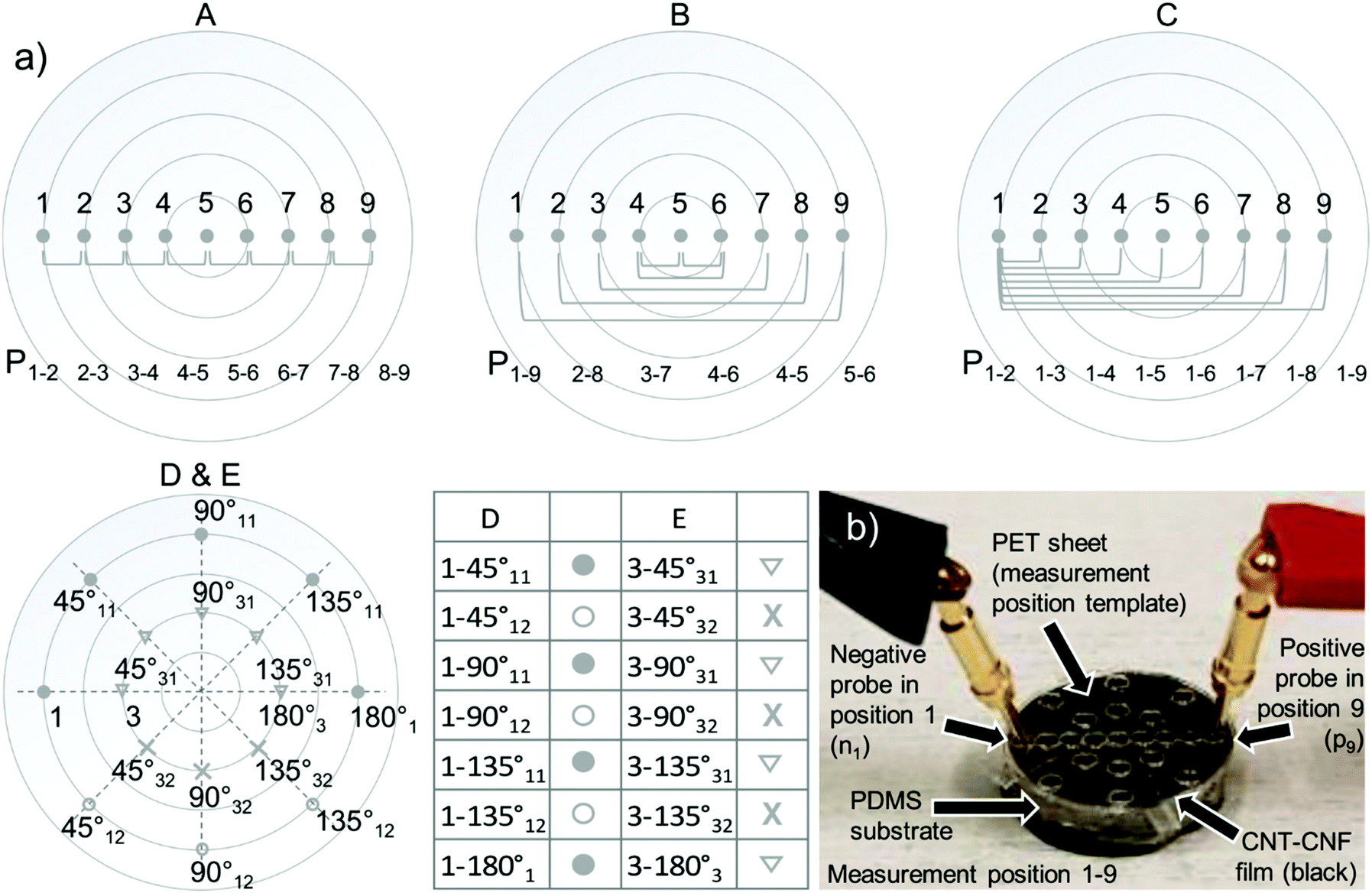Fig. 8 Resistance measurement protocol (a) and measurement setup (b). Measurements A–C are performed along the centre line, while measurements D and E follow circle 1 (D) and circle 3 (E) according to the measurement protocol presented in measurements A–E (a), respectively. Measurement locations for measurements A–C are presented in the corresponding map, while the measurement locations for measurements D and E are shown in the table next to the D & E map.

Electron microscopy. Scanning electron microscopy (SEM) and (scanning) transmission electron microscopy ((S)TEM) were used to characterize the nanomaterials used and nanocomposite films. Front and side views of the nanocomposite films were characterized using SEMs (UltraPlus, Carl Zeiss, Oberkochen, Germany; JSM-IT500, Jeol Ltd, Tokyo, Japan). The samples were attached to aluminum SEM stubs using carbon tape or carbon glue. The front view was imaged on the surface of the nanocomposite films, while the side view was characterized from the torn film edges. Torn films were placed between a string and fixed on the SEM stub to obtain a cross-section and edge views of the films. The samples were either carbon or gold-coated to avoid charging during the SEM studies. (S)TEM (JEM-F200, Jeol Ltd, Tokyo, Japan) was used to characterize the nanomaterials used and nanocomposite films. Untreated MWCNTs and small pieces of torn nanocomposite film edges were fixed on TEM grids with a holey carbon film.

Alignment characterization. SEM images were collected at different locations on the film to perform SEM image-based orientation analysis. Cytospectre software³³ was used for the analysis. A parameter called circular variance (CV) was determined from each image in order to describe to degree of orientation. A CV value of 1 refers to perfect isotropy, while a value of 0 is perfect anisotropy. In addition to the CV value, a mean orientation angle of each image location was determined in order to show the orientation direction along the evaporating boundary line. While CV only describes the degree of orientation – that is, isotropy or anisotropy – the mean orientation can be used to show if the orientation direction is according to our hypothesis; that is, along the evaporation boundary line, and thus along the imaginary circles.

MicroCT. Nanocomposite films were imaged with X-ray microtomography (microCT) using MicroXCT-400 (X-ray tube voltage of 40 kV and a current of 250 μA; Carl Zeiss X-ray Microscopy, Inc., Pleasanton, CA, USA). The imaged sample area was 2.98 mm². 3D microCT images were reconstructed from 1601 projections with a 10 s exposure time (20× objective, binning 2, pixel size 1.048 μm) using the microCT software tool XMReconstructor. 3D image stacks were manually thresholded for the 3D analysis. The mean film thickness with standard deviations from different locations of the films was calculated with the BoneJ Fiji plugin.⁴⁵ The data visualization was realized using Avizo 2019.3 software (Thermo Fisher Scientific, Waltham, MA, USA).

Atomic force microscopy. Atomic force microscopy scanning was performed in a tapping mode using a standard ACTA AFM probe with a resolution of 256 × 256 pixels. Images were analyzed and postprocessed using AFM image processing software XEI (Park Systems, USA).

Nuclear magnetic resonance spectroscopy (NMR). The following samples were prepared and freeze-dried for NMR studies. The cationic CNF hydrogel (2.01 w%) was diluted to 0.15 w% (W/v) concentration in D₂O (Sigma Aldrich), sample 1 (untreated c-CNF). Samples 2–4 were sonicated for 2 min at 20% amplitude using a SONICS Vibra Cell VCX 750 ultrasonic processor (Sonics and Materials, Inc., USA), with subsequent centrifugation at 10 000g for 60 min (Thermo Scientific SL 8). The resulting supernatant was sonicated using 625 kJ g⁻¹ or 1250 kJ g⁻¹ and a tip horn sonicator Q700 (QSonica LLC, Newton, CT, USA), resulting in samples 2 and 3 (c-CNF supernatant sonicated 625 kJ g⁻¹ or 1250 kJ g⁻¹, respectively). Sample 4 (sonicated c-CNF-MWCNT dispersion) was prepared by sonicating the c-CNF supernatant (in D₂O) and MWCNTs using 625 kJ g⁻¹. Samples 1–4 were freeze-dried to remove excess moisture and used in NMR experiments.

NMR spectra were measured on a 500 MHz JEOL JNM-ECZ 500R spectrometer. Samples (approx. 50 mg) were packed into 3.2 mm diameter zircônia rotors with KelF caps as a tick suspension in D₂O. The semi-solid state FG-MAS ¹H spectra were recorded at room temperature, with the high-resolution field gradient FG-MAS probe at a spinning rate of 5 kHz. A water suppression pulse sequence was applied during the measurements.

Conclusions

Application of sonochemical treatments to aqueous mixtures of cationic nanofibrillated cellulose and carbon nanotubes leads to even and relatively stable solutions of the assembled components, which can be easily formed as free-standing conductive nanocomposite films. Diverse characterization techniques confirm the strong interactions between c-CNFs and CNTs, mainly occurring through ionic and hydrophobic interactions, as well as hydrogen bonding induced by sonochemical treatments. Sonochemical treatment induces robust interactions between c-CNFs and MWCNTs in aqueous media, forming a strong entangled hybrid nanoparticle dispersion hes-c-CNF/MWCNT, where cationic functional groups of hes-c-CNFs point outwards from the hybrid structure. Drying of the dispersion results in evenly conducting films, while the incorporation of free c-CNFs (S1, S2) or hes-c-CNFs (S3) makes it possible to control the self-assembly of nanomaterials along the evaporating dry-line boundary and the simultaneous formation of conducting zones and thus the directional increase in resistance in the radial direction. The amount and composition of the added c-CNFs (or hes-c-CNFs) influence the conductivity differences in different directions. These films can be considered as free-standing self-assembled nanocomposite films displaying a tunable surface with functional properties such as adjustable conductivity. The novelty in the method described herein is that it produces adjustable directional conductivity and uses c-CNFs as a dispersing agent. The method is not limited to a specific application or to nanocomposite films as a substrate. Instead, the tunable composition, substrate preparation technique, and functionalization possibilities offer interesting possibilities in the fields of biomedical sciences and energy applications in general and should be studied further.

Author contributions

The manuscript was written through contributions of all authors. All authors have given approval to the final version of the manuscript.

Conflicts of interest

There are no conflicts of interest to declare.

Acknowledgements

We acknowledge K. Tornberg for casting PDMS sheets for substrate preparation, M. Jokinen for his technical help related to laser cutting of the measurement template, and M. Kakkonen for his technical help with IR imaging. SEM and (S)TEM studies were carried out at Tampere University using Tampere Microscopy Center facilities. We acknowledge P. Willberg-Keyriläinen (Senior Scientist, VTT) for the cationization of CNFs.

References

1. H. Zhang, C. Dou, L. Pal and M. A. Hubbe, BioResources, 2019, 14, 7494–7542.
2. K. Li, C. M. Clarkson, L. Wang, Y. Liu, M. Lamm, Z. Pang, Y. Zhou, J. Qian, M. Tajvidi, D. J. Gardner, H. Tekinalp, L. Hu, T. Li, A. J. Ragauskas, P. Youngblood and S. Ozcan, ACS Nano, 2021, 15, 3646–3673.
3. Q. Zhu, Q. Yao, J. Sun, H. Chen, W. Xu, J. Liu and Q. Wang, Carbohydr. Polym., 2020, 230, 115609.
4. C. Zamora-Ledezma, C. Blanc, N. Puech, M. Maugey, C. Zakri, E. Anglaret and P. Poulin, Phys. Rev. E, 2011, 84, 1–5.
5. S. Siljander, P. Keinänen, A. Ivanova, J. Lehmonen, S. Tuukkanen, M. Kanerva and T. Björkqvist, Materials, 2019, 12, 430.
6. S. Siljander, P. Keinänen, A. Räty, K. R. Ramakrishnan, S. Tuukkanen, V. Kunnari, A. Harlin, J. Vuorinen and M. Kanerva, Int. J. Mol. Sci., 2018, 19, 1–14.
7. A. Hajian, S. B. Lindström, T. Pettersson, M. M. Hamedi and L. Wåberg, Nano Lett., 2017, 17, 1439–1447.
8. Z. Shi, G. O. Phillips and G. Yang, Nanoscale, 2013, 5, 3194–3201.
9. M. Bhattacharya, M. M. Malinen, P. Lauren, Y. R. Lou, S. W. Kuisma, L. Kanninen, M. Lille, A. Corlu, C. Guguen-Guillouzo, O. Ikkala, A. Laukkanen, A. Urtti and M. Yliperttula, J. Controlled Release, 2012, 164, 291–298.
10. Y.-R. Lou, L. Kanninen, T. Kuisma, J. Niklander, L. A. Noon, D. Burks, A. Urtti and M. Yliperttula, Stem Cells Dev., 2014, 23, 380–392.
11. M. M. Malinen, L. K. Kanninen, A. Corlu, H. M. Isoniemi, Y. R. Lou, M. L. Yliperttula and A. O. Urtti, Biomaterials, 2014, 35, 5110–5121.
12. L. Alexandrescu, K. Syverud, A. Gatti and G. Chinga-Carrasco, Cellulose, 2013, 20, 1765–1775.
13. M. Čolić, D. Mihajlović, A. Mathew, N. Naseri and V. Kokol, Cellulose, 2015, 22, 763–778.
14. K. Hua, E. Ålander, T. Lindström, A. Mihranyan, M. Strømme and N. Ferraz, Biomacromolecules, 2015, 16, 2787–2795.
15. Z. Wang, D. O. Carlsson, P. Tammela, K. Hua, P. Zhang, L. Nyholm and M. Strømme, ACS Nano, 2015, 9, 7563–7571.
16. A. Lekawa-Raus, J. Patmore, L. Kurzepa, J. Bulmer and K. Koziol, Adv. Funct. Mater., 2014, 24, 3661–3682.
17. A. B. Fall, S. B. Lindström, O. Sundman, L. Ödberg and L. Wågberg, Langmuir, 2011, 27, 11332–11338.
18. P. T. Hammond, Adv. Mater., 2004, 16, 1271–1293.
19. A. Olszewska, P. Eronen, L. S. Johansson, J. M. Malho, M. Ankerfors, T. Lindström, J. Ruokolainen, J. Laine and M. Österberg, Cellulose, 2011, 18, 1213.
20. Y. Xue, Z. Mou and H. Xiao, Nanoscale, 2017, 9, 14758–14781.
21. V. Thakur, A. Guleria, S. Kumar, S. Sharma and K. Singh, Mater. Adv., 2021, 2, 1872–1895.
22. A. Skogberg, A. J. Mäki, M. Mettänen, P. Lahtinen and P. Kallio, Biomacromolecules, 2017, 18, 3936–3953.
23. Y. A. J. Al-Hamadani, K. H. Chu, A. Son, J. Heo, N. Her, M. Jang, C. M. Park and Y. Yoon, Sep. Purif. Technol., 2015, 156, 861–874.
24. C. Salas, T. Nypelö, C. Rodriguez-Abreu, C. Carrillo and O. J. Rojas, Curr. Opin. Colloid Interface Sci., 2014, 19, 383–396.
25. P. Keinänen, S. Siljander, M. Koivula, J. Sethi, E. Sarlin, J. Vuorinen and M. Kanerva, Heliyon, 2018, 4, e00787.
26. M. M. Hamedi, A. Hajian, A. B. Fall, K. Hkansson, M. Salajkova, F. Lundell, L. Wgberg and L. A. Berglund, ACS Nano, 2014, 8, 2467–2476.
27. J. B. Mougel, C. Adda, P. Bertoncini, I. Capron, B. Cathala and O. Chauvet, J. Phys. Chem. C, 2016, 120, 22694–22701.
28. C. Olivier, C. Moreau, P. Bertoncini, H. Bizot, O. Chauvet and B. Cathala, Langmuir, 2012, 28, 12463–12471.
29. H. Koga, T. Saito, T. Kitaoka, M. Nogi, K. Suganuma and A. Isogai, Biomacromolecules, 2013, 14, 1160–1165.
30. I. Lavilla and C. Bendicho, in Water Extraction of Bioactive Compounds, Elsevier Inc., 2017.
31. D. Yang, J.-F. Rochette and E. Sacher, J. Phys. Chem. B, 2005, 109, 7788–7794.
32. M. Mashkour, T. Kimura, F. Kimura, M. Mashkour and M. Tajvidi, Biomacromolecules, 2013, 15, 60–65.
33. K. Kartasalo, R.-P. Pölönen, M. Ojala, J. Rasku, J. Lekkala, K. Aalto-Setälä and P. Kallio, BMC Bioinf., 2015, 16, 344.
34. L. M. Mariani, G. S. Vankayalapati, J. M. Conisidine and K. T. Turner, in Mechanics of Biological Systems and Materials & Micro-and Nanomechanics, Springer, Cham, 2019.
35. T. Pöhler, T. Lappalainen, T. Tammelin, P. Eronen, P. Hiekkataipale, A. Vehniäinen and T. Koskinen, in TAPPI International Conference on Nanotechnology ForestProduct Industry, 2010, pp. 437–458.
36. B. Lindman, G. Karlström and L. Stigsson, J. Mol. Liq., 2010, 156, 76–81.
37. G. Jia, H. Wang, L. Yan, X. Wang, R. Pei, T. Yan, Y. Zhao and X. Guo, Environ. Sci. Technol., 2005, 39, 1378–1383.
38. V. Pérez-Luna, C. Moreno-Aguilar, J. L. Arauz-Lara, S. Aranda-Espinoza and M. Quintana, Sci. Rep., 2018, 8, 1–11.
39. C. M. Voge, M. Kariolis, R. A. MacDonald and J. P. Stegemann, J. Biomed. Mater. Res., Part A, 2008, 86, 269–277.
40. P. S. Goh, A. F. Ismail and B. C. Ng, Composites, Part A, 2014, 56, 103–126.
41. L. Bacakova, J. Pajorova, M. Tomkova, R. Matejka, A. Broz, J. Stepanovska, S. Prazak, A. Skogberg, S. Siljander and P. Kallio, Nanomaterials, 2020, 10, 1–32.
42. J. Pajorova, A. Skogberg, D. Hadraba, A. Broz, M. Travnickova, M. Zikmundova, M. Honkanen, M. Hannula, P. Lahtinen, M. Tomkova, L. Bacakova and P. Kallio, Biomacromolecules, 2020, 21, 4857–4879.
43. D. Kai, M. P. Prabhakaran, G. Jin and S. Ramakrishna, J. Biomed. Mater. Res., Part B, 2011, 98, 379–386.
44. J. Bendoraitiene, R. Kavaliauskaite, R. Klimaviciute and A. Zemaitaitis, Starch/Staerke, 2006, 58, 623–631.
45. A. Palmroth, S. Pitkänen, M. Hannula, K. Paakinaho, J. Hyttinen, S. Miettinen and M. Kellomäki, J. R. Soc., Interface, 2020, 17, 20200102.

---

Footnotes

† Electronic supplementary information (ESI) available: Additional experimental details and results. See DOI: 10.1039/d1nr06937c

‡ These authors contributed equally.

---