
Plasmons: untangling the classical, experimental, and quantum mechanical definitions
Rebecca L. M.
Gieseking

Department of Chemistry, Brandeis University, 415 South Street, Waltham, Massachusetts 02453, USA. E-mail: gieseking@brandeis.edu; Tel: +1-781-736-2511
First published on 28th September 2021
Abstract
Plasmons have been widely studied over the past several decades because of their ability to strongly absorb light and localize its electric field on the nanoscale, leading to applications in spectroscopy, biosensing, and solar energy storage. In a classical electrodynamics framework, a plasmon is defined as a collective, coherent oscillation of the conduction electrons of the material. In recent years, it has been shown experimentally that noble metal nanoclusters as small as a few nm can support plasmons. This work has led to numerous attempts to identify plasmons from a quantum mechanical perspective, including many overlapping and sometimes conflicting criteria for plasmons. Here, we shed light on the definitions of plasmons. We start with a brief overview of the well-established classical electrodynamics definition of a plasmon. We then turn to the experimental features used to determine whether a particular system is plasmonic, connecting the experimental results to the corresponding features of the classical electrodynamics description. The core of this article explains the many quantum mechanical criteria for plasmons. We explore the common features that these criteria share and explain how these features relate to the classical electrodynamics and experimental definitions. This comparison shows where more work is needed to expand and refine the quantum mechanical definitions of plasmons.
 Rebecca L. M. Gieseking | Rebecca Gieseking earned her PhD in Chemistry from Georgia Tech in 2015. After three years as a postdoctoral fellow at Northwestern University, she started her independent career as an Assistant Professor at Brandeis University in 2018. Her research interests focus on developing low-cost quantum mechanical models to understand electron transfer processes in materials for emerging photochemical and electrochemical energy technologies. |
1. Introduction
Since Michael Faraday discovered in 1856 that solutions of colloidal gold nanoparticles have a bright red color,1 the optical properties of metal nanostructures have fascinated scientists. The origins of the unique optical properties resulting from the quantized oscillations of a free electron gas (plasma) were proposed by Pines and Bohm in the early 1950s2–4 and became known as plasmons (or plasmon resonances). Plasmons have been widely studied over the past several decades because of their ability to strongly absorb light and localize its electric field on the nanoscale,5–7 leading to applications in spectroscopy,8–11 biosensing,11–13 and solar energy conversion.14–18 Although the noble metals gold and silver have been the most widely studied for their plasmonic properties, the field of plasmonics has expanded to encompass a broad range of materials, including other metals like magnesium and aluminum,19,20 doped semiconductors,21,22 and organic materials like graphene.23,24Much of the research in plasmonics has focused on nanoparticles and nanostructures on the order of tens to hundreds of nm, which have been widely modeled using classical electrodynamics.25,26 In recent years, there has been great interest in the emergence of plasmonic properties in noble metal nanoclusters on the scale of ∼1–3 nm, or ∼10–500 metal atoms.27–31 New synthetic techniques have made it possible to synthesize hundreds of unique nanoclusters with atomically precise structures similar to those of molecules,27,32–35 and many of these nanoclusters have been characterized using techniques like X-ray crystallography.36–38 Because the structures are atomically precise, the observed optical properties and excited-state dynamics reflect the individual properties of one specific structure, instead of being averaged over a distribution of similar structures with slightly different properties. Many of these nanoclusters are also small enough to study using quantum mechanical models, giving detailed insight into their properties.39–41 As these developments have converged, there have been many distinct but overlapping definitions proposed for how to identify plasmons within a quantum mechanical framework,42–49 which has led to confusion in the field.
The purpose of this Focus Article is to shed light on the definitions and key features of plasmons within three different frameworks: (1) classical electrodynamics, (2) experimental spectroscopic characterization, and (3) quantum mechanics. The classical electrodynamics and quantum mechanical frameworks are usually explained using different terminology; for readers who are new to the field, a brief overview of the connections between these two sets of terminology is included in the Appendix. We start with a brief overview of the classical electrodynamics view of plasmons. We then turn to the experimental spectroscopic features that are used to determine whether a particular system is plasmonic, focusing on connecting the experimental results to the corresponding features of the classical electrodynamics description. The remainder of this Focus Article will explain approaches to identify plasmons in a quantum mechanical context. Since there are many overlapping definitions of plasmons within a quantum mechanical framework, this section will go into the most depth, and will focus on exploring the common features that these definitions share and explaining how these features relate to the classical electrodynamics and experimental definitions. This comparison will show where more work needs to be done to expand and refine the quantum mechanical definitions of plasmons. Because plasmonics is a broad field, the scope of this article is deliberately limited to noble metals and to dipolar plasmons, though many of the concepts are straightforward to extend.
2. Classical electrodynamics view of plasmons
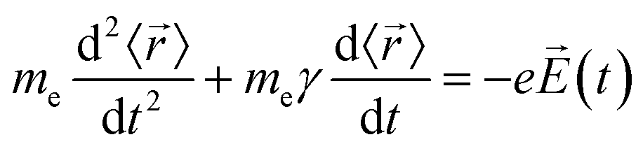
The description of plasmons from a classical electrodynamics perspective is well established, and many previous reviews have gone into extensive detail.26,50–52 Since the main goal of this Focus Article is to connect the classical, experimental, and quantum mechanical descriptions, we focus here on highlighting the features of the classical model that are most important to understanding the experimental and quantum mechanical descriptions in the later sections. Because metals have no band gap, the conduction electrons can travel freely throughout the metal in response to an electric field, leading to their high electrical conductivity. These conduction electrons can be thought of as being analogous to a plasma, or a free electron gas. The electrons in this plasma can only oscillate at certain quantized frequencies; these quantized oscillations are called plasmons.The frequencies of these plasmonic oscillations are related to the dielectric constant of the metal, which can be derived from the Drude model.51,53,54 Within the Drude model, the nuclei are fixed, and the conduction electrons are treated as classical particles that move in response to their interactions with the time-dependent electric field ![[E with combining right harpoon above (vector)]](https://www.rsc.org/images/entities/i_char_0045_20d1.gif) (t) and with other electrons. The electrons follow the equation of motion
(t) and with other electrons. The electrons follow the equation of motion
 | (1) |
![[r with combining right harpoon above (vector)]](https://www.rsc.org/images/entities/i_char_0072_20d1.gif) 〉 is the average electron position, me is the electron mass, e is the elementary charge, and γ is a material-specific damping term related to electron–electron repulsion that is sometimes referred to as friction. The first term is mass × acceleration, and the term on the right side is the force on the electron.
〉 is the average electron position, me is the electron mass, e is the elementary charge, and γ is a material-specific damping term related to electron–electron repulsion that is sometimes referred to as friction. The first term is mass × acceleration, and the term on the right side is the force on the electron.
Since plasmons are related to electron oscillations, we will focus on oscillating electric fields that correspond to the electric field of light with frequency ω, such that (t) = 0e−iωt. Under this electric field, the average electron position will oscillate with the same frequency, such that 〈(t)〉 = 〈0〉e−iωt. Plugging these two equations into the equation of motion, we obtain
 | (2) |
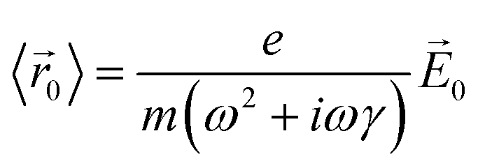 | (3) |
![[P with combining right harpoon above (vector)]](https://www.rsc.org/images/entities/i_char_0050_20d1.gif) 0 = −Ne〈0〉, where N is the number of conduction electrons per unit volume. Thus, the polarization in response to the electric field is:
0 = −Ne〈0〉, where N is the number of conduction electrons per unit volume. Thus, the polarization in response to the electric field is: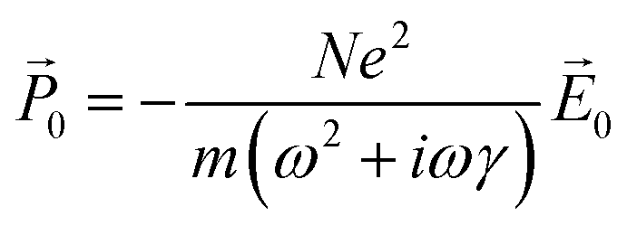 | (4) |
| 0 = ε0(ε(ω) − 1)0 | (5) |
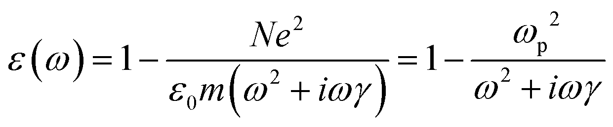 | (6) |
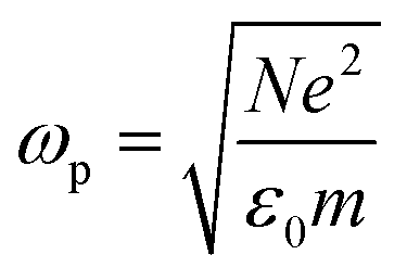 is the plasma frequency, which is an inherent material property. Most metals have plasma frequencies in the ultraviolet.
The dielectric constant can be related to the optical properties of the material via the refractive index 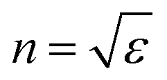 . The phase velocity of light through a material
 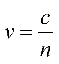 , where c is the speed of light in a vacuum. Most non-metals have refractive indices >1, indicating that light travels more slowly through the material than through vacuum. In metals, there are three ranges of frequencies of light that are important:
1. ω < ωp: in this regime (which includes the visible range for most metals), Re(ε) < 0 and n is imaginary. The electric field light decays exponentially inside the metal, so the metal reflects light.
2. ω > ωp: in this regime, 0 < Re(ε) < 1 and 0 < n < 1, and the metal is transparent. This transparency is seen experimentally within the UV for alkali metals.55 Although the phase velocity of light through the material is larger than c, the phase of light does not carry information, so this does not violate relativity.
3. ω = ωp: at this frequency, Re(ε) = 0 and n = 0. The phase velocity is infinite, which means that the electrons oscillate in phase throughout the material, resulting in a plasmon. At the same frequency, Im(ε) is positive and relatively large, indicating strong absorption.
Because the Drude model only includes the conduction electrons, it neglects interband transitions, which have a positive contribution to both the real and imaginary parts of ε that can be added as an empirical correction:
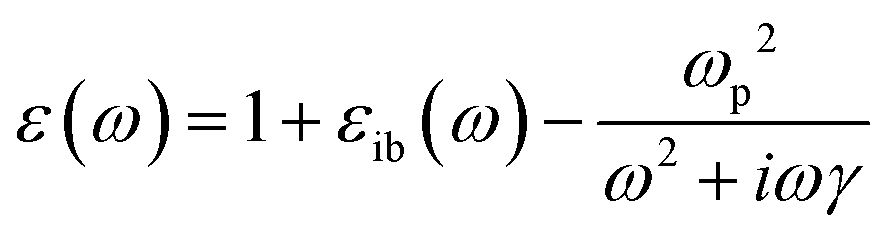 | (7) |
To this point, we have focused on the optical response of bulk metals, leading to quantized oscillations in the bulk metal known as bulk plasmons. Plasmons may also occur at an extended interface between a metal and another material, referred to as surface plasmons. For this article, we are most interested in plasmons in discrete metal nanoparticles or nanoclusters, known as localized surface plasmons (or localized surface plasmon resonances, LSPRs). The finite size of the nanoparticle will affect the frequency at which the localized surface plasmon is observed.
The optical response of spherical nanoparticles can be computed using Mie theory,51,52,56 which is an analytical solution to Maxwell's equations. For most non-spherical nanostructures, Maxwell's equations must be solved using numerical techniques.25,57,58 Because we are interested in nanoparticles and nanoclusters that are much smaller than the wavelength of light, we can approximate that the electric field of light is uniform across the entire nanoparticle (quasistatic approximation), which simplifies the equations. The displacement of the electrons in response to the electric field of light creates an instantaneous buildup of electrons on one side of the nanoparticle and depletion of electrons on the other side (Fig. 14d), creating an internal electric field with magnitude
 | (8) |
 | (9) |
The key result from these electrodynamics models is that metal nanoparticles have strong plasmon resonances that result from an oscillation of the conduction electrons. This oscillation is collective among all the conduction electrons and is coherent, meaning that the electrons are oscillating in the same direction at the same time. The strong oscillation of the electrons is also associated with strong absorption of light at the resonant frequency.
3. Experimental view of plasmons
In the past several decades, new synthetic approaches have produced hundreds of distinct atomically precise noble metal nanoclusters coated with a ligand shell, ranging in size from tens to hundreds of metal atoms.27,32–35 Depending on the size, shape, metal composition, and ligands, these nanoclusters may exhibit either plasmonic or excitonic properties. Spectroscopic studies have shown that there are features that distinguish plasmonic from excitonic behavior in two main areas: (1) the instantaneous optical properties and (2) the dynamics following absorption. This section does not cover every experimental distinction between plasmonic and excitonic systems, which have been reviewed more extensively elsewhere.63–66 Instead, we focus on two main goals: (1) relating the key features that are seen experimentally to their classical electrodynamics explanation, and (2) laying the necessary groundwork so that it is clear in the next section what similarities and differences exist between the properties used experimentally vs. in quantum mechanical models to distinguish between plasmonic and excitonic behavior.The first distinguishing feature of plasmonic behavior is the absorption spectrum, reflecting the instantaneous response of the nanocluster to light. As seen from the classical electrodynamics model, because plasmons are collective oscillations, a (nearly) spherical plasmonic nanocluster should have only one peak in its absorption spectrum, as seen for 22 nm Au nanoparticles in Fig. 1a. In contrast, excitonic nanoclusters may have several or many absorption peaks involving transitions between different molecular orbitals, such as that of the Au6(PPh3)62+ nanocluster in Fig. 1b. In larger nanoclusters, the transition from an excitonic multi-peaked absorption spectrum to a single-peaked plasmonic absorption spectrum is visible as the nanocluster size increases from Au246(SR)80 to Au279(SR)84,30 though overlap of the intraband and intraband transitions somewhat obscures the intraband absorption peaks (Fig. 1c).
 | ||
| Fig. 1 Absorption spectra of (a) plasmonic 22 nm Au spherical nanoparticles (adapted from ref. 67), (b) excitonic Au6(PPh3)62+ nanoclusters (adapted from ref. 68), (c) Au246(SR)80 and Au279(SR)84 nanoclusters showing a transition from excitonic to plasmonic behavior (adapted from ref. 30). | ||
Several spectroscopic techniques that probe the dynamics following absorption also reveal differences between excitonic and plasmonic behavior. To understand the reasons for these differences, we must first examine the typical decay processes. When plasmonic metal nanoparticles absorb light, the initially coherent plasmon dephases into individual hot charge carriers (hot electrons and hot holes) within a few femtoseconds (Fig. 2).69–71 The initial distribution of hot carriers is relatively uniform over a broad range of energies.72–74 Because the electron–electron scattering rate is higher for charge carriers farther from the Fermi energy, the higher-energy charge carriers lose energy more quickly than the lower-energy carriers.75–77 This scattering transforms the initial non-thermal hot carrier distribution into a thermal distribution within a few hundred femtoseconds, in a process called thermalization.78–80 On the scale of a few ps, the hot carriers relax, and the excess energy is transferred into phonons.74,81–83
 | ||
| Fig. 2 Schematic of non-radiative plasmon decay processes, including dephasing into hot electrons and holes on the order of 10 fs, thermalization of hot carriers within 100–500 fs, and relaxations of hot carriers into phonons within 1–10 ps. | ||
In contrast, the decay of excitonic systems depends on the specific electronic excited states in the nanocluster. In the prototypical Au nanocluster Au25(SR)18−, three distinct decay time scales have been measured,84 though the details of the decay depend on the exact ligand structure, the excitation energy, and other experimental factors.27 First, the hot carriers within the metal core relax within several hundred fs.84–86 This is followed by transfer of energy from the metal core to states with ligand-to-metal charge-transfer character within a few ps84 and relaxation to vibrational modes on the order of 50–200 ns.84,87 These time scales are several orders of magnitude larger than for similar decay processes in plasmonic systems. Unlike in typical plasmonic systems, higher-energy excited states in excitonic nanoclusters may have longer lifetimes than the low-energy excited states of the same nanocluster.85 Because there are discrete excited states, decay from one state to another occurs on a distinctive time scale, and that time scale varies between different nanocluster isomers88 or sizes.89
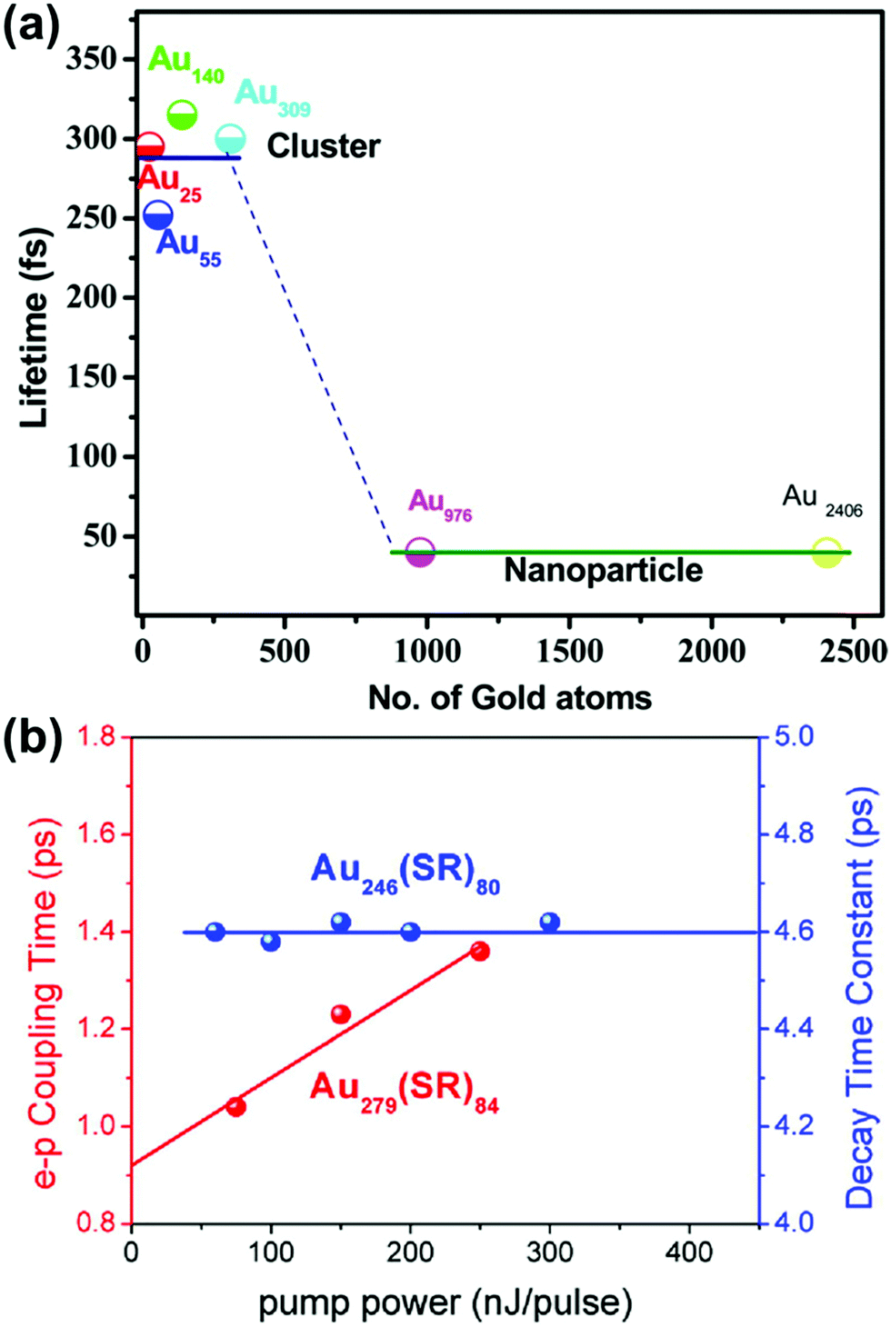
Because of the differences in the excited-state dynamics, plasmonic and excitonic noble metal nanoclusters have distinct emission mechanisms and time scales.63,90 Both classes of nanoclusters typically have two emissive transitions: a short-lived visible emission attributed to the decay of an excitation in the nanocluster core, and a longer-lived near-infrared emission attributed to ligand states.36,85,91 For the shorter-lived visible emission, plasmonic gold nanoparticle have fluorescence lifetimes <50 fs, which is faster than can be resolved experimentally; this rapid decay reflects the fast dephasing and thermalization processes (Fig. 3a). In contrast, excitonic gold nanoclusters have visible fluorescence time scales on the order of 250–350 fs, reflecting the slower decay from the initial excited states into ligand states.90
 | ||
| Fig. 3 (a) Fluorescence lifetimes of gold nanoclusters of various sizes, showing a transition from long excitonic lifetimes to short plasmonic lifetimes; adapted from ref. 90. (b) Electron–phonon coupling time scales extracted from transient absorption data for the excitonic Au246(SR)80 and the plasmonic Au279(SR)84; adapted from ref. 30. | ||
The differences in the decay processes of excitonic and plasmonic gold nanoclusters can also be observed in differences in the pump-power dependence of their decay time scales, as observed by various time-resolved spectroscopic techniques.85,92–96 For plasmonic nanoclusters and nanoparticles, the time scale of the relaxation of electronic energy into phonons depends on the intensity of the pump laser used to excite the system: because a high pump power can cause one nanoparticle to absorb multiple photons, the initial hot carriers have a higher effective temperature, and these higher-energy hot carriers decay more quickly. In contrast, in excitonic nanoclusters, the relaxation time scale is independent of the pump power because the excitation and decay processes involve discrete excited states that decay with their own distinctive time scales. In thiol-protected Au nanoclusters, a sharp transition from excitonic to plasmonic dynamics is seen as the size increases from Au246(SR)80 to Au279(SR)84 (Fig. 3b).30 However, the transition from excitonic to plasmonic behavior is not simply a function of nanocluster size: the smaller nanocluster Au144(SR)60 has plasmonic pump-power dependence.96
4. Quantum mechanical view of plasmons
Atomistic quantum mechanical methods can practically be applied to systems on the scale of tens to hundreds of atoms. Thus, unlike metal nanoparticles with diameters larger than 2–3 nm, many atomically precise nanoclusters are within a size range that can be studied using quantum mechanical methods to understand their geometries, optical properties, and dynamics with atomistic detail. The majority of the quantum mechanical calculations in the field have used density functional theory (DFT) approaches, but other computational methods like INDO97–99 and density functional tight binding (DFTB)100–103 give results that are largely consistent with DFT.Early calculations using time-dependent DFT (TD-DFT) showed that bare tetrahedral silver nanoclusters have relatively sharp absorption peaks similar to those characteristic of plasmonic nanoparticles that red-shift with increasing size, and extrapolation of the absorption energy to larger sizes yields results consistent with electrodynamics for plasmonic systems.42 Based on these early observations, there has been great interest in using quantum mechanical calculations to understand the emergence of plasmonic properties and in developing techniques to characterize whether nanoclusters have plasmonic or excitonic properties.43,44,46,47,104,105 These different characterization methods focus on various aspects of the definition of plasmons from classical electrodynamics, and in some cases multiple characterization approaches attempt to quantify similar aspects of the electrodynamics definition. Here, we summarize the main characterization techniques and then focus on their application to prototypical linear metal nanowires, which are widely used as model systems.
We note that the characterization methods described here all focus on the static excited states computed by frequency-domain methods like TD-DFT or the absorption spectra obtained from time-domain methods like real-time TD-DFT (RT-TDDFT). There have been some computational studies of the excited-state dynamics using RT-TDDFT on the time scale of dephasing106–108 and non-adiabatic molecular dynamics (NAMD) on the time scale of relaxation.109–111 However, criteria to distinguish between excitonic and plasmonic states based on the dynamics are much less developed at this point.
4.1. Oscillatory behavior
As discussed earlier, the electrodynamics description of plasmons involves an oscillation of the electron density. However, when excited states are computed using frequency-domain quantum mechanical methods, the states that are obtained are stationary states, meaning that the electron density is constant over time. At a first glance, it may appear that quantum mechanical excited states could never represent the oscillatory behavior inherent to plasmons. However, this apparent contradiction is straightforward to resolve by instead considering time-domain quantum mechanical methods. Since the electrodynamics derivation of plasmonic behavior involves a time-dependent electric field, a time-dependent quantum mechanical method involving an electric field with explicit time dependence allows for a more direct comparison.Frequency-domain excited-state methods like linear-response TD-DFT compute a list of excited eigenstates ψk, along with their corresponding energy eigenvalues Ek and transition dipole moments 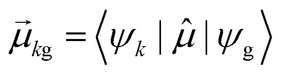 . The absorption intensity from the ground state ψg to excited state ψk is proportional to
 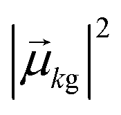 . This yields a “stick spectrum” where each excited state is represented by a stick with a height corresponding to the absorption intensity. To obtain an absorption spectrum that more closely resembles an experimental spectrum, each stick is broadened using a Lorentzian or Gaussian function, and the intensities are summed to give one total absorption spectrum.
Time-domain quantum mechanical methods apply an electric field as a time-dependent perturbation to the system and compute the evolution of the wavefunction over time. The time-dependent electric field may be a wavepacket with a sinusoidal shape over a finite time; it may also be a delta function where an electric field is applied for only a single time step that, via a Fourier transform, is equivalent to exciting the system with a broad distribution of frequencies. We will focus here on excitation with a sinusoidal wavepacket with a small enough intensity that the system remains mostly in the ground state. In the time domain, absorption can be described using first-order time-dependent perturbation theory, which we describe briefly here; the full derivation can be found in many quantum mechanics textbooks. Within this framework, the Hamiltonian is:
Ĥ = Ĥ(0) + Ĥ′(t) = Ĥ(0) − F0![[small mu, Greek, circumflex]](https://www.rsc.org/images/entities/i_char_e0b3.gif) ![[thin space (1/6-em)]](https://www.rsc.org/images/entities/char_2009.gif) sinωt sinωt | (10) |
; is the dipole operator. The time-dependent wavefunction can be written as a linear combination of the eigenfunctions ψ(0)k of the unperturbed system: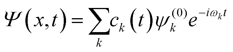 | (11) |
 | (12) |
 , the coefficient ck(t′) will be non-zero, indicating that the system has absorbed light to transition from Ψ(0)g to Ψ(0)k. The probability of a transition from the ground state to state ψk is proportional to |ck(t′)|2 and thus is also proportional to
  . If there are no decay processes, the coefficients ck(t′) remain constant in magnitude after the electric field is turned off. If ω is not close to resonance with the transition from Ψ(0)g to Ψ(0)k, the coefficient ck(t′) remains small.
The resulting time-dependent wavefunction is a superposition of the ground-state wavefunction with a small coefficient for the resonant excited-state wavefunction Ψ(0)k:
| Ψ(t) = e−iωgt(cgψg + ckψke−iωgkt) | (13) |
 | (14) |
The crucial result is that any strongly absorbing state, whether plasmonic or excitonic, has a large transition dipole moment, leading to large oscillations of the instantaneous dipole moment in the time domain that continue until a decay process occurs. An example of these dipole oscillations for the icosahedral Ag55 nanocluster is shown in Fig. 4; in this case, the electric field is on for approximately the first 10 fs, and decay processes lead to significant damping of the oscillations between 20 and 25 fs.106 A large transition dipole moment is necessary for an excited state to yield the large time-dependent charge oscillations characteristic of plasmons. However, large charge oscillations cannot be the only characteristic used to determine whether an excited state is plasmonic or excitonic, since every strongly absorbing state will induce large charge oscillations in the time domain. Thus, more criteria are needed to distinguish strongly absorbing plasmonic excited states from strongly absorbing excitonic excited states.
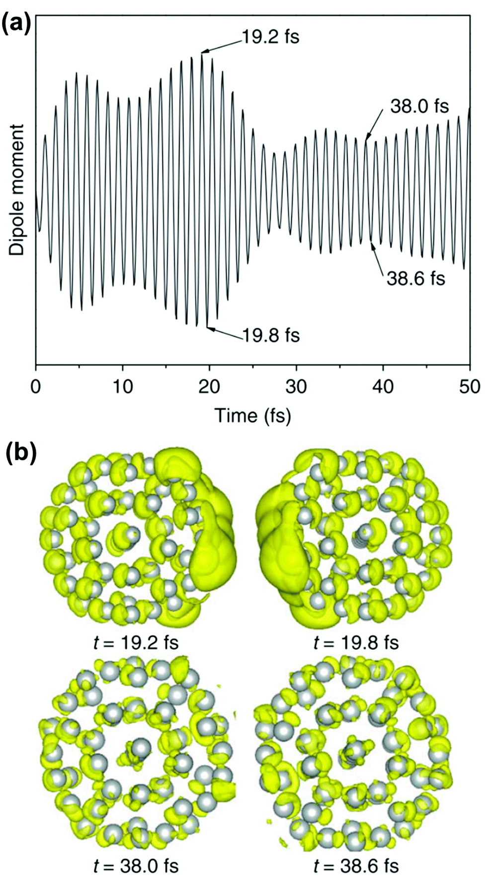 | ||
| Fig. 4 (a) Time-dependent dipole moment of Ag55 in RT-TDDFT simulations where the system is excited with 3.6 eV light for the first 10 fs of the simulation. (b) Charge density differences at select time steps, showing large charge oscillations at early times. Adapted from ref. 106. | ||
We first focus on distinguishing factors directly related to the nature of the charge oscillations. Early analysis of plasmonic nanospheres found that the absorption peaks can be classified into two categories based on the spatial distribution of the charge oscillations.104,112 Some absorption peaks are associated with large charge oscillations that are primarily localized near the nanocluster surface and involve excitations of electrons from just below to just above the Fermi energy; these peaks that involve large “sloshing” of the electron density were called classical surface plasmons. In contrast, other absorption peaks are due to charge oscillations primarily near the nanocluster core and involve higher-energy single-particle excitations; these peaks were termed quantum core plasmons.
More quantitative approaches to analyzing the electron oscillations have also been developed. As described in the classical electrodynamics section, the large oscillation of the conduction electrons in a plasmon creates a large internal electric field inside the nanoparticle. One approach to identify plasmons is based on quantifying these internal (or induced) electric fields.45,46,113 In the limit of an infinite homogeneous system, the frequency-dependent induced charge distribution δn(k, ω) is
| δn(k, ω) = χ0(k, ω)vtot(k, ω) = χ0(k, ω)[vext(k, ω) + vind(k, ω)] | (15) |
 | (16) |
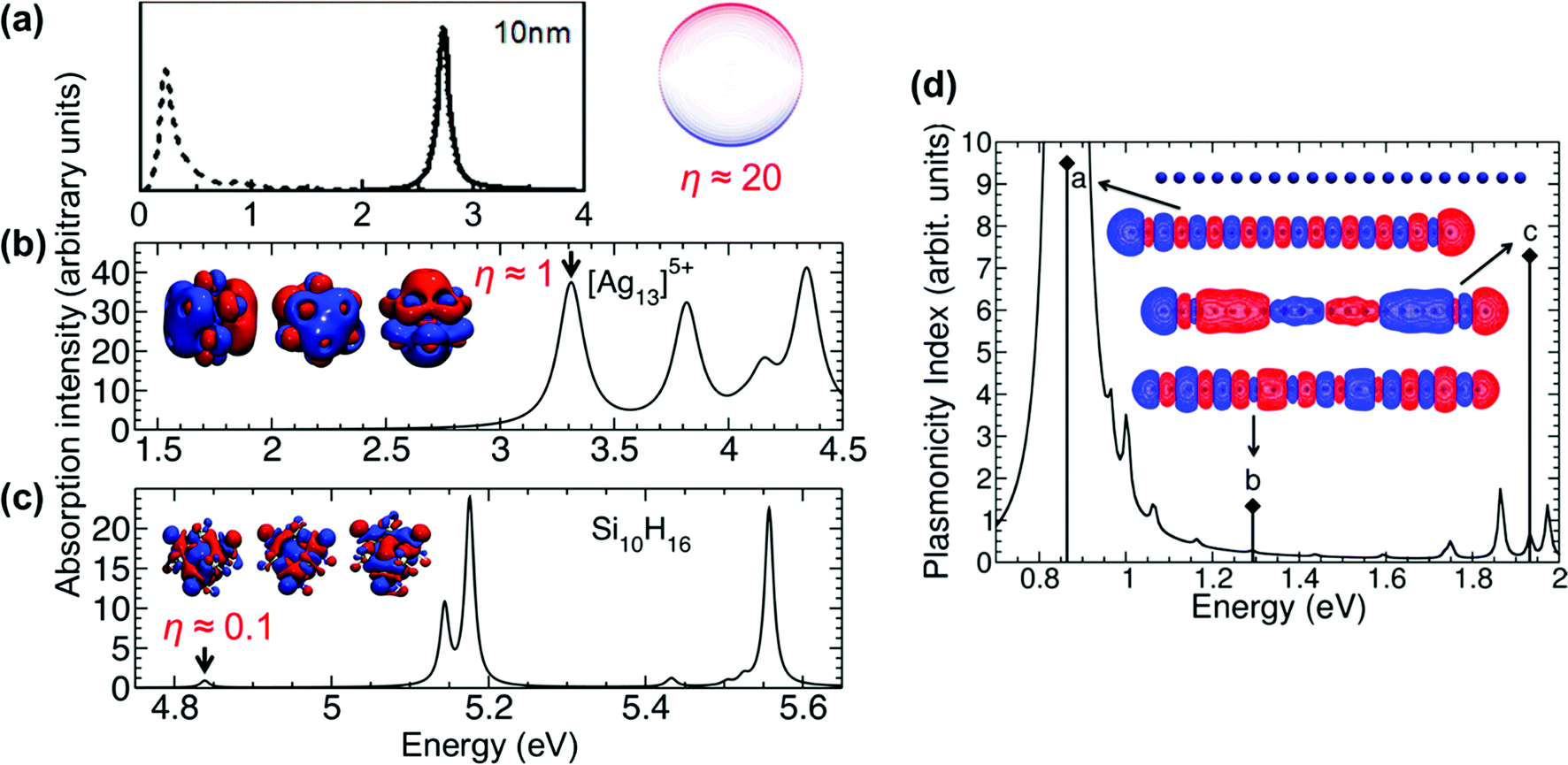 | ||
| Fig. 5 Absorption spectra, transition densities, and generalized plasmonicity indices (GPIs) of the indicated absorption peaks for (a) a plasmonic 10 nm Au sphere, (b) Ag135+, and (c) the non-plasmonic Si10H16 cluster; adapted from ref. 45. (d) Absorption spectrum, transition densities, and plasmonicity indices of the indicated absorption peaks for a Na20 nanowire; adapted from ref. 46. | ||
4.2. Conduction-band character
From the Drude model, we saw that plasmons are oscillations of the metal conduction-band electrons. By translating the terminology of band theory into the terminology of molecular orbital (MO) theory, it is relatively straightforward to identify which MOs correspond to the conduction band based on their AO character. In most metal nanoclusters, the low-lying unoccupied MOs are part of the conduction band, so analyses typically focus only on the occupied MOs.The most straightforward way to identify the MOs corresponding to the conduction band is to identify the MOs that are composed primarily of the valence s and p AOs (5s and 5p for Ag, 6s and 6p for Au). Since each excited state k is a linear combination of excitations from occupied to unoccupied MOs, the overall contribution of conduction-band electrons CBk can be quantified as a sum of the contributions from the occupied MO involved each excitation:
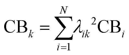 | (17) |
Because of this limitation, a more practical approach to identify the conduction-band electrons is via the superatomic MOs.114 This approach has been widely used to understand the electronic and optical properties of noble metal nanoclusters.115–118 The name ‘superatomic’ refers to the fact that these MOs have shapes that (in roughly spherical metal clusters) resemble the shapes of atomic orbitals, but are delocalized across the entire metal cluster. The superatomic MOs are composed primarily of the valence sp AOs, and thus correspond to the conduction-band electrons. Each superatomic MO is labeled with a number equal to (# radial nodes +1) and an upper-case letter indicating its angular momentum (S, P, D, F, G,…). This labeling scheme is slightly different than atomic orbital nomenclature: for example, the 1P superatomic MO has a shape that resembles a 2p atomic orbital, the 2P MO resembles the 3p AO, and the 1D MO resembles the 3d AO. The low-lying superatomic orbitals for the icosahedral Ag135+ nanocluster are shown in Fig. 6a; this nanocluster has 8 conduction-band electrons filling the 1S and 1P superatomic MOs. The Aufbau rule for filling of superatomic shells is 1S2|1P6|1D10|2S2 1F14|2P6 1G18|2D10 3S2 1H22|….114
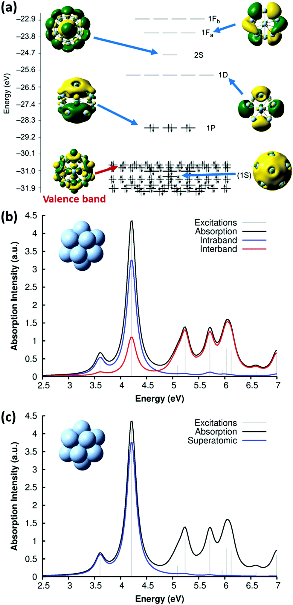 | ||
| Fig. 6 (a) Molecular orbital energies and isosurfaces for Ag135+; adapted from ref. 119. Absorption spectrum of Ag135+ at the SAOP/TZP level of theory, decomposed into (b) intraband vs. interband and (c) superatomic character; adapted from ref. 43. | ||
The contribution of superatomic electrons Sk to excited-state k can be computed as
 | (18) |
4.3. Collectivity and coherence
In early quantum mechanical calculations of the excited states of Ag and Au clusters, it was observed that the strongly absorbing excited states involve a linear combination of several to many single-particle excitations.42 We can understand this in a simplified way by examining a prototypical system that has a ground state ψg with energy Eg = 0 and three single-particle excitations ϕ1, ϕ2, and ϕ3, each with energy α and transition dipole moment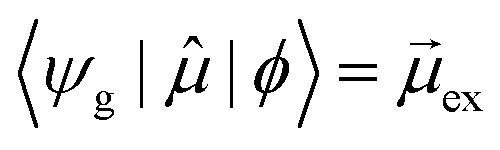 .120 Each pair of single-particle excitations has a coupling of β. For this prototypical system, the excited states are the eigenvectors of the configuration interaction (CI) matrix
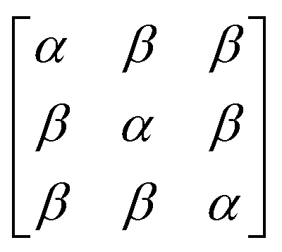 | (19) |
 | (20) |
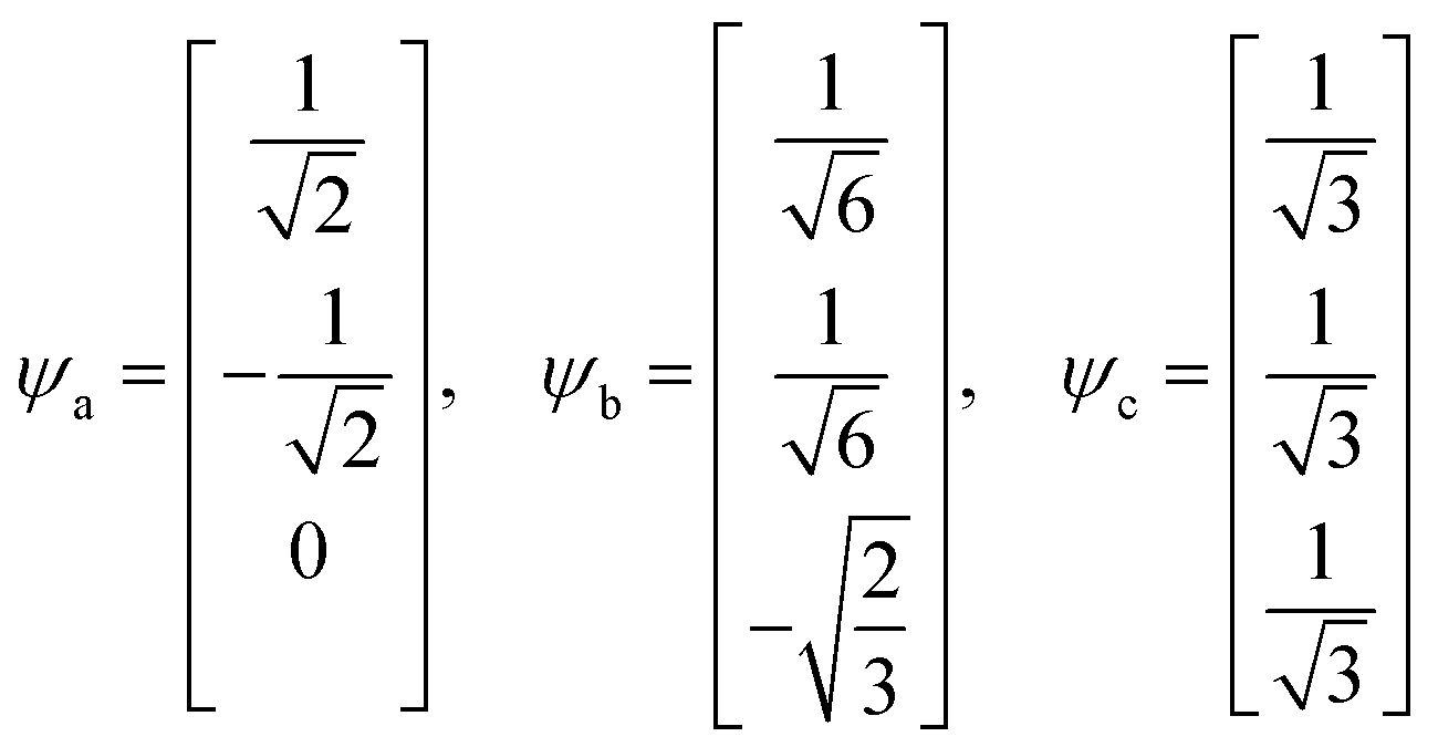
| Ea = Eb = α − β, Ec = α + 2β | (21) |
For excited state ψa, the transition dipole moment 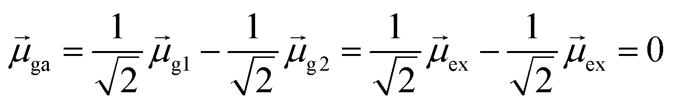 . Similarly,
 ![[small mu, Greek, macron]](https://www.rsc.org/images/entities/i_char_e0cd.gif) gb = 0. Even though the component single-particle excitations are absorbing states, mixing these states results in cancellation of their transition dipole moments, resulting in optically dark states. In contrast,
gb = 0. Even though the component single-particle excitations are absorbing states, mixing these states results in cancellation of their transition dipole moments, resulting in optically dark states. In contrast, 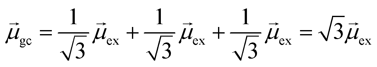 . Thus, the absorption intensity of excited state ψc is proportional to
 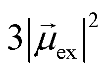 , or equivalent to the sum of the absorption intensities of the three component single-particle excitations. Coupling of the excitations causes the absorption to be redistributed into only the highest energy state, shifting the absorption to higher energy than the component single-particle excitation energies. This additive coupling of the single-particle excitations is roughly equivalent to the plasmonic coherence of all of the conduction electrons oscillating in the same direction at the same time. In addition to the collective, coherent, plasmonic excited states, the same system has other excited states that are linear combinations of some or all of the same single-particle excitations that involve cancellation of the transition dipole moments, which are not plasmonic.
Several methods of quantifying plasmonic character have focused on different features that are shown in this simple model: (1) the number of single-particle excitations that contribute to an excited state, (2) the addition or cancellation of the contributions of the component single-particle excitations to the transition dipole moment, and (3) the correlation between the energies and coupling of single-particle excitations on the excited-state energy.
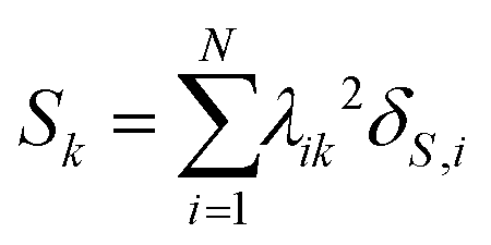
The collectivity can be quantified by computing the number of single-particle excitations contributing to an excited state via the transition inverse participation ratio (TIPR) τk,44 computed as
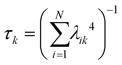 | (22) |
 for both single-particle excitations, and thus
 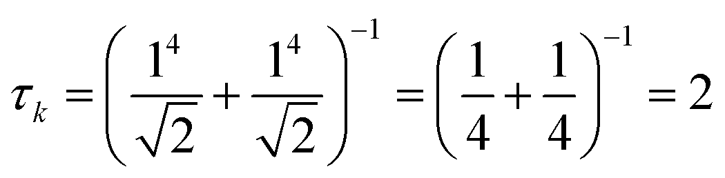 . Similarly, for any excited state that is composed of N single-particle excitations with equal weights, τk = N. If the weights of the N single-particle excitations are instead unequal, 1 < τk < N. Thus, τk gives an estimate of the number of single-particle excitations that mix to form excited-state k. In metal nanoclusters, the main absorbing states with large superatomic character often have large τk.43,44 However, as can be seen in Fig. 7, there are also many excited states with large τk that do not strongly absorb light. Because of the large density of states in the valence band or in occupied ligand bands, the excited states with largest τk are typically excited states with primarily intraband character,43 so high collectivity cannot be used as the sole criterion to determine which excited states are plasmonic.
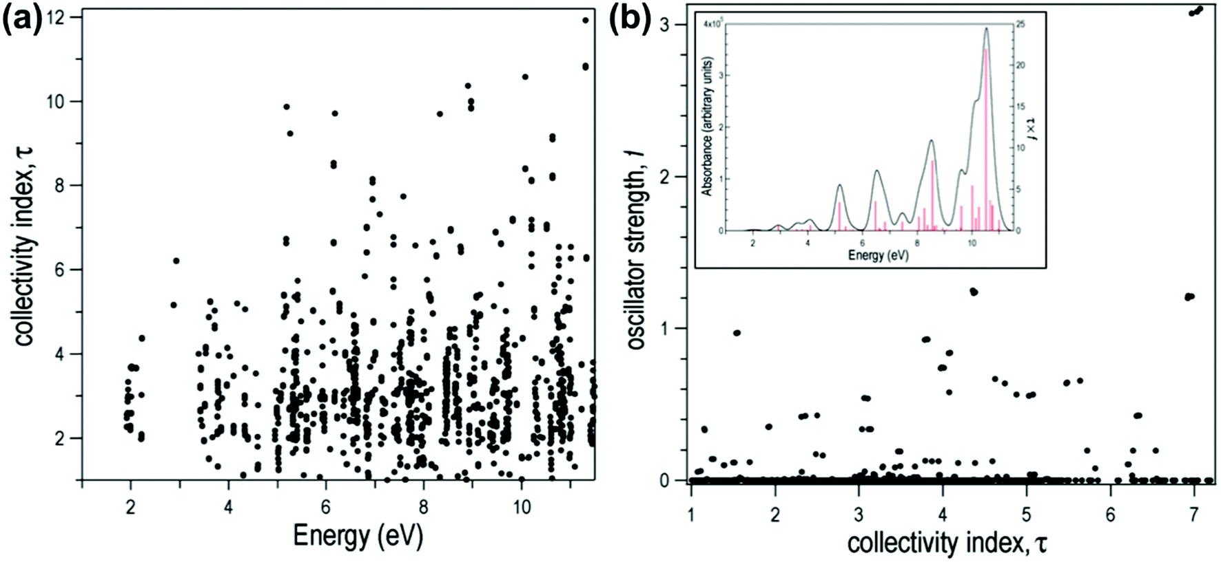 | ||
| Fig. 7 Collectivity (τ) of the excited states of the icosahedral Al13− as a function of (a) excited-state energy and (b) oscillator strength. Inset: Computed absorption spectrum of Al13−. Adapted from ref. 44. | ||
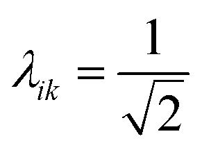
Thus, other approaches are needed to identify which of the highly collective excited states have the coherence typical of plasmons. One approach to quantify coherence is via the additivity of the single-particle excitation contributions to the transition dipole moment gk of each excited state.43,97 The dipole additivity dk is computed as
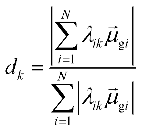 | (23) |
 terms, similar to the two non-absorbing states in the CI model above) to 1 (perfect additivity of terms, similar to the one absorbing states in the CI model). Excited states with large
  tend to have relatively large dk values; however, a small
  may occur either because dk is small or because the excited state is composed of excitations with small
  values. In addition, states with small collectivity typically to have large dk, since only one excitation has a large contribution to
  .
.
For prototypical bare and ligand-protected silver nanoclusters, the collectivity (TIPR), dipole additivity, and superatomic character are nearly orthogonal.43 Since plasmons are collective, coherent oscillations of the conduction electrons, all three criteria must be large for an excited state to be plasmonic. None of these criteria are sufficient on their own, but in combination they can indicate whether or not a particular excited state is plasmonic.
A related approach to identify plasmonic excited states is by visualizing the excitations that contribute to each excited state in a transition contribution map (TCM);105,121 this decomposition approach has also been extended to time-domain methods.122 In these maps, each excitation corresponds to a spot with x and y coordinates corresponding to the energies of the occupied and virtual orbitals involved in the excitation, respectively, and the intensity of the spot corresponds to the weight of the excitation (Fig. 8). The TCM for a collective excited state has many spots with similar intensity, whereas the TCM for an excited state with low collectivity will have one or a few intense spots. For collective excited states, the spatial distribution of the spots also gives information about the coupling among the single-particle excitations. In the CI model system at the beginning of this section, the large coupling between excitations means that the absorbing state has a higher energy than its component single-particle excitations, and a larger coupling leads to a larger energetic shift. Similarly, in the TCM, a plasmonic excited state involving strong coherent coupling between excitations will tend to have a higher energy than its component excitations. Thus, if an excited state is plasmonic, its TCM should have several to many spots corresponding to transitions with energies below the excited-state energy.
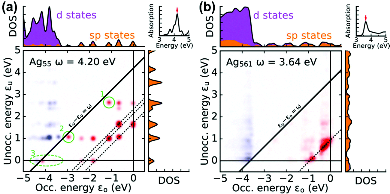 | ||
| Fig. 8 Transition contribution maps for the main absorption peaks in icosahedral (a) Ag55 and (b) Ag561 nanoclusters; adapted from ref. 122. Red spots and blue spots indicate contributions from transitions that are lower or higher in energy than the energy of light, respectively. | ||
A related characterization method is based on quantifying the energy distribution of excitations contributing each excited state, resulting in an energy-based plasmonicity index (EPI).47 This index is based on the off-diagonal density matrix elements ρωmn coupling electron configurations m and n for an excited state with energy ω within a time-dependent framework. The elements ρωmn are essentially equivalent to the weights of excitations λmn within a frequency-domain framework. The raw density matrix elements are rescaled as
 | (24) |
![[small rho, Greek, tilde]](https://www.rsc.org/images/entities/i_char_e0e4.gif) ωmn is much larger than ρωmn for excitations nearly equal in energy to the incoming light and smaller for off-resonance transitions. Based on these density matrix elements, the EPI is computed as:
ωmn is much larger than ρωmn for excitations nearly equal in energy to the incoming light and smaller for off-resonance transitions. Based on these density matrix elements, the EPI is computed as: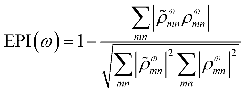 | (25) |
ω to ρω. For a single-particle excitation, only one element ρωmn is non-zero, so the second term in EPI(ω) is equal to 1. For a plasmonic state, many excitations ρωmn have non-zero contributions; if these states have a large distribution of energies, ωmn and ρωmn will be relatively different and the second term in EPI(ω) will approach zero.
A final approach to identify plasmonic excited states is similarly based on couplings between the single-particle excitations. In TD-DFT, it is possible to scale all of the couplings between single-particle excitations by a factor λ that ranges from 0 (yielding excited states that are identical to uncoupled single particle excitations) to 1 (standard TD-DFT). Excited states that are composed primarily of one single-particle excitation have relatively constant energies as λ is scaled, whereas excited states composed of strongly coupled single-particle excitations increase in energy with increasing λ.48,49 One challenge in applying this method is that a large number of TDDFT calculations must be performed to trace the energetic evolution of each excited state; this approach is also challenging to apply to large systems with relatively large densities of excited states.
4.4. Plasmonic properties of linear metal nanowires
Linear nanowires have been widely used as prototypical systems to test the criteria for plasmons described in the previous sections. We will end with a comparison of how the main excited states in these nanowires are classified based on these criteria. To perform these comparisons, we must first overview the electronic structures of these nanowires. Linear nanowires composed of either noble metals or alkali metals have one electron per atom in a MO corresponding to the metal conduction band. All of the occupied conduction-band MOs are σ bonding orbitals composed primarily of the metal valence s orbitals; the number of nodes perpendicular to the long axis of the nanowire ranges from 0 to , where N is the number of atoms. These MOs are typically given the names Σn, where n is one greater than the number of long-axis nodes. The LUMO is a σ-type orbital with
  nodes, and there are higher-energy unoccupied MOs with π-type character with the names Πn (Fig. 9a).
 | ||
| Fig. 9 (a) Molecular orbital diagram and (b) absorption spectrum of the linear Ag8 nanowire at the SAOP/TZP level (data from ref. 98). | ||
The nanowires have two major absorption peaks at relatively low energies (Fig. 9b), one corresponding to a longitudinal excitation (transition dipole moment oriented along the long axis of the nanowire) and one corresponding to a transverse excitation (transition dipole moment oriented perpendicular to the nanowire long axis). The longitudinal peak results from an excited state that primarily involves a transition from HOMO to LUMO (Table 1), and its energy is approximately inversely proportional to the number of metal atoms.107,123,124 The transverse peak is relatively constant in energy with increasing nanowire length and is composed of a linear combination of excitations from Σ-type to Π-type MOs. At some levels of theory, the transverse peak in silver nanowires also includes a non-negligible contribution from interband transitions.107,123,124 We will examine the behavior of these nanowires in the context of various schemes to identify which (if either) of these absorption peaks have plasmonic character. The results of these analyses are summarized in Table 2.
| Energy (eV) | Major transitions | Oscillator strength | Superatomic character | Collectivity | Dipole additivity |
|---|---|---|---|---|---|
| 1.521 | Σ4 → Σ5 (89.7%; 0.61 eV) | 2.014 | 99.5% | 1.23 | 84.7% |
| Σ2 → Σ5 (7.9%; 1.35 eV) | |||||
| 6.295 | Σ2 → Π4 (23.1%; 6.07 eV) | 0.702 | 79.2% | 8.18 | 47.3% |
| Σ4 → Π4 (16.4%; 5.32 eV) | |||||
| Σ1 → Π1 (10.7%; 5.01 eV) | |||||
| Σ2 → Π2 (10.3%; 5.09 eV) | |||||
| Σ3 → Π3 (9.7%; 5.21 eV) | |||||
| Σ3 → Π5 (9.7%; 6.53 eV) |
| QM analysis | Property measured | Nanowire(s) studied | Plasmonic character | |
|---|---|---|---|---|
| Longitudinal | Transverse | |||
| Plasmonicity index46 | Internal electric field | Na20 | High | — |
| Superatomic character | Conduction band | Ag8 | High | Moderate to high |
| Transition inverse participation ratio | Collectivity | Ag8 | Low | High |
| Dipole additivity | Coherence | Ag8 | N/A | Moderate |
| Transition contribution map | Collectivity, energy distribution | Ag8 | Mixed | High |
| Energy-based plasmonicity index47 | Energy distribution | M70 | Moderate to high | — |
| Lambda scaling49 | Coupling between excitations | Na20 | High | — |
We start with the criteria based on electron density oscillations. The generalized plasmonicity index (GPI) described earlier has not been applied to nanowires to date; however, an earlier formulation called the plasmonicity index (PI) was applied to the longitudinal excited states of the Na20 nanowire (Fig. 5d).46 Because the longitudinal absorption peak has large positive transition density on one end of the nanowire and large negative transition density on the other end, the internal electric field is large, and thus the plasmonicity index is large. However, other weakly absorbing states also have comparably large plasmonicity indices, which suggests that a large plasmonicity index may not be sufficient to call a particular excited state plasmonic. Since this version of the plasmonicity index depends on system size, it is challenging to interpret the numerical values, and no plasmonicity indices were presented for the transverse states.
The next criterion is the bands contributing to each excited state. For nanowires, the AO-based terminology for superatomic MOs is not applicable because the nanowires are far from spherical; however, the Σ and Π MOs composed primarily of the Ag 5s and 5p AOs can be considered superatomic-like MOs corresponding to the conduction band. For the prototypical nanowire Ag8, the longitudinal peak has nearly 100% superatomic character. In contrast, the transverse peak has primarily superatomic character, but also has approximately 20% interband character (Table 1).98 As described previously, a large superatomic character is necessary but not sufficient for an excited state to be classified as plasmonic.
The collectivity and coherence can be quantified via the TIPR and dipole additivity. For the example of the Ag8 nanowire, the longitudinal excited state is primarily a single-particle transition (HOMO → LUMO), and so the collectivity is very close to 1 (Table 1). Because one excitation dominates, the dipole additivity must be relatively large; thus, the large dipole additivity cannot be used as an indicator of plasmonic character. The low collectivity suggests that the longitudinal state may not be plasmonic. In contrast, the transverse excited state has much higher collectivity because of the contributions of multiple Σ → Π transitions. The dipole additivity is lower than for the longitudinal state, but is still larger than that of the excited states in larger nanoclusters.99 Thus, the transverse state better satisfies this pairing of plasmonic criteria than the longitudinal state.
The transition contribution maps (TCMs) visualize the energy distribution and weights of the excitations that contribute to each excited state. For the Ag8 nanowire (Fig. 10), since the longitudinal excited state is essentially a HOMO → LUMO transition, there is only one large spot in the TCM, which is consistent with the low collectivity. However, this spot is at an orbital energy difference 0.9 eV lower than the excited-state energy. This indicates that the small amount of mixing with other excitations significantly affects the excited-state energies, which may indicate that this excited state has some plasmon-like characteristics. In contrast, the transverse excited state has several spots with similar weight indicating significant contributions from several excitations, and the excitations with the largest weights have orbital energy differences lower than the excited-state energy. Both of these features indicate plasmonic character.
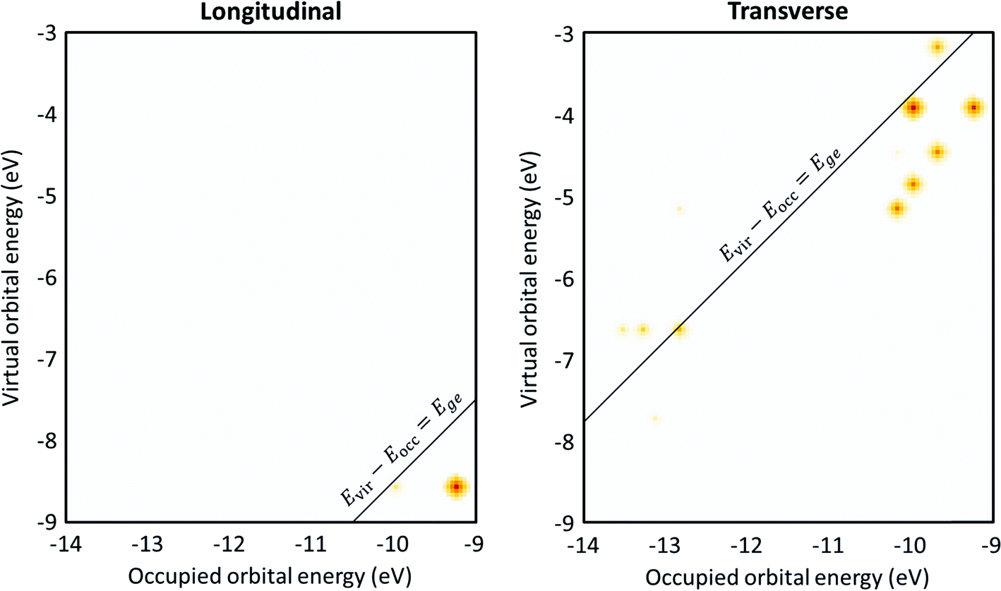 | ||
| Fig. 10 Transition contribution maps (TCMs) for the (left) longitudinal and (right) transverse excited states of Ag8. Data is from ref. 98. | ||
The energy-based plasmonicity index (EPI), which quantifies the distribution of the excitations contributing to an excited state, has been applied to the longitudinal excited states of a 70 atom nanowire within a tight-binding model.47 This model includes only the conduction electrons and uses an empirical coupling between neighboring atoms; electron–electron repulsion is neglected. Because of these simplifications, the model predicts a series of longitudinal absorption peaks (Fig. 11). The first of these peaks is equivalent to the longitudinal excited state computed in the other models. In a neutral nanowire, this peak has a moderate EPI, indicating moderate plasmonic character. When the nanowire is doped by adding additional electrons, the EPI increases. This plasmonic indicator was not used for the transverse excited states.
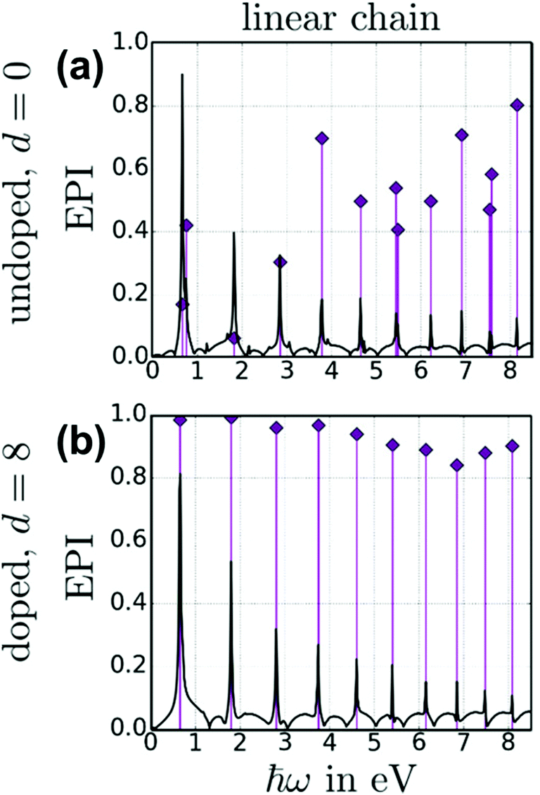 | ||
| Fig. 11 Absorption spectrum (black lines) and energy-based plasmonicity index (EPI; purple diamonds) for a 70 atom nanowire within a tight-bonding model, comparing (a) a neutral undoped nanowire to (b) a nanowire doped with 8 electrons. Adapted from ref. 47. | ||
 | ||
| Fig. 12 (left) Effect of the scaling of the electronic interaction on the excited state energies of the linear Na20 nanowire. (right) Absorption spectrum of Na20 and transition densities of the excited states identified as plasmons. Adapted from ref. 49. | ||
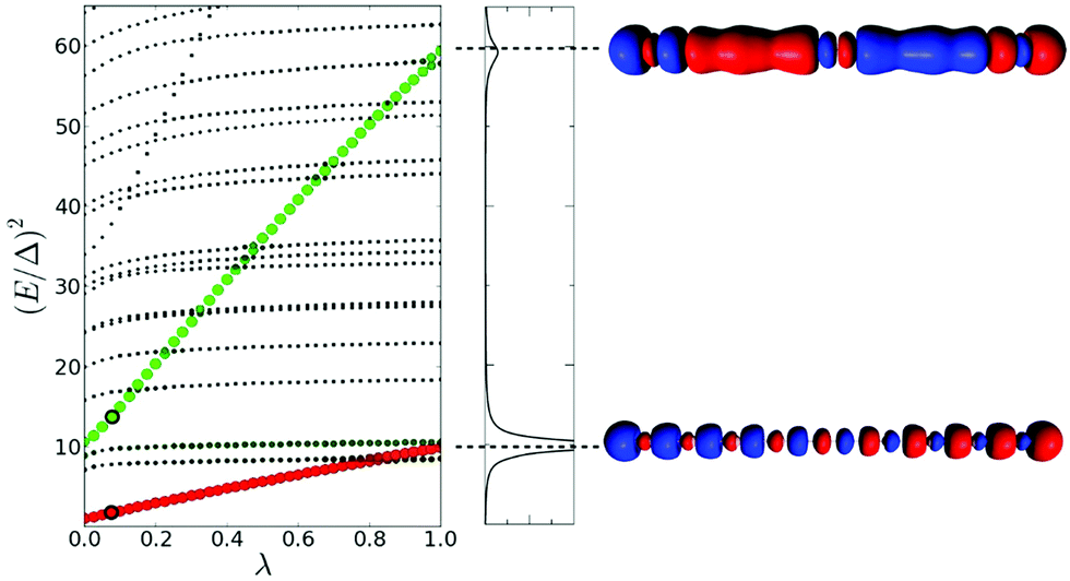
The lambda scaling approach based on the effect of coupling on the excited state energies has been applied to the longitudinal excited states of the Na20 nanowire (Fig. 12).49 The first longitudinal absorption peak is due to an excited state that shows a large increase in energy as the coupling between excitations increases, which is an indicator of plasmonic character. This is consistent with the large energy difference seen in the TCM between the energy of the HOMO → LUMO transition and the first excited state energy. This analysis was not applied to the transverse excited states.
By directly comparing these criteria for identifying plasmonic states, it is clear that they do not give entirely consistent results about which excited states are plasmonic. For linear nanowires, both the longitudinal and transverse excited states have primarily conduction-band character. The longitudinal excited state satisfies some but not all of the criteria for plasmons. The internal electric field is large, and the energy difference between the HOMO → LUMO transition and the excited state is large. However, this excited state is essentially a single-particle transition, so it is not collective and thus cannot be coherent. In contrast, the transverse excited state has much higher collectivity and reasonably large coherence, but many of the other plasmonic criteria have not been tested for this state. These discrepancies highlight the need for more work to define consistent criteria for plasmons and determine what criteria best reflect the features used experimentally to determine whether states are plasmonic.
5. Synopsis
Understanding the transition from excitonic to plasmonic properties in noble metal nanoclusters is important to enhance their properties for applications such as sensing and photocatalysis. The original definition of a plasmon stems from classical electrodynamics, and this framework has been used widely to understand the properties of plasmonic nanoparticles and nanoclusters. Within this model, a material with conduction electrons will have specific resonant frequency at which collective, coherent oscillation of the conduction electrons occur, which is defined as a plasmon. This is in contrast with an exciton, which is a bound electron–hole pair.Experimentally, distinguishing plasmonic systems from excitonic systems requires examining the optical properties and dynamics. Plasmonic systems typically have a single absorption peak at the resonant oscillation frequency of the electron gas, whereas excitonic systems typically have more complex absorption spectra. The differences in the dynamics following absorption derive from differences between the rapid decay processes for plasmonic systems with a continuum of states and the slower decay processes for excitonic systems with discrete states. Experimentally, thiol-protected gold nanoclusters transition from excitonic to plasmonic at sizes on the order of several hundred metal atoms.
Quantum mechanical approaches to distinguish between plasmonic and excitonic excited states have focused to date largely on the instantaneous excited states upon absorption. Because plasmons emerge in ligand-protected gold nanoclusters at large enough sizes that they are challenging to study using quantum mechanical methods, most quantum mechanical analyses of plasmonic character have focused on systems like bare silver nanoclusters where plasmonic behavior emerges at smaller sizes. The difference between the systems studied experimentally and quantum mechanically makes it somewhat challenging to evaluate to what extent the quantum mechanical methods are capturing properties that correlate with experimental observations.
Many quantum mechanical criteria have been developed to identify plasmons, and most of the individual criteria are designed to evaluate one aspect of the description of plasmons that emerges from electrodynamics. The criteria encompass a broad range of plasmonic properties, including the spatial distribution of the charge oscillations, the conduction-band character of the electrons involved in the excited state, the collectivity and coherence of the various single-particle excitations that contribute to the excited state, and the strength of the coupling between the single-particle excitations that contribute to the excited state. Since individual criteria may be nearly orthogonal, a particular excited state may need to satisfy several of these criteria to be classified as plasmonic. In addition, these criteria may yield contrasting results for the same system. For example, the main longitudinal absorption peaks of linear nanowires are classified as plasmonic using some but not all of the criteria; the main transverse absorption peaks satisfy all of the plasmonic criteria that have been used to analyze them, but a number of criteria have not yet been applied to these states.
More work remains to understand which of these criteria yield results that best correlate with the emergence of plasmonic behavior experimentally. Since many of these criteria have been used only for bare nanoclusters to date, extension to ligand-protected nanoclusters may introduce new challenges. In addition, since many of the experimental properties used to distinguish plasmons are based on the excited-state dynamics, more work is needed to understand whether these criteria correlate with distinctive changes in the dynamics. Refining the quantum mechanical definition of plasmons has the potential to play a significant role in understanding structure–property relationships in metal nanoclusters and in tuning their properties for applications throughout the field of plasmonics.
Appendix: basic terminology
Because plasmonics bridges the fields of chemistry, physics, and materials science, there are multiple overlapping sets of terminology that are used. Depending on the size of metal nanoclusters and nanoparticles, the electronic structure may be described in the language of either molecular orbital theory, typically used for discrete molecules, or band theory, commonly used for extended systems (Fig. 13). As atoms combine to form molecules and small nanoclusters, their atomic orbitals (AOs) overlap and mix to form discrete molecular orbitals (MOs) at specific energies. The most significant of these are the highest occupied and lowest unoccupied MOs, HOMO and LUMO. As the system increases in size, the number of MOs scales proportionally to the number of atoms. For very large systems, the number of MOs becomes so large that they form a near continuum. The MOs in an extended system can be grouped into sets with very similar character, known as bands. Some bands may overlap in energy; in other energy ranges, there may be energy gaps between bands where there are no MOs, known as band gaps. In insulators and semiconductors, the valence band is the highest-energy band that is fully occupied, and the conduction band is the lowest-energy empty band; insulators have large band gaps between the valence and conduction band, and semiconductors have smaller band gaps between these two bands. In contrast, in a metal, one band is partly occupied, so there is no band gap. For noble metals, the partially occupied band composed of the valence sp atomic orbitals (5s and 5p for Ag, 6s and 6p for Au) is called the conduction band (or sp band), and the fully occupied band composed of d orbitals (4d for Ag, 5d for Au) is called the valence band (or d band). Because “valence” refers to different sets of orbitals in each framework, translating between these two sets of terminology must be done with care.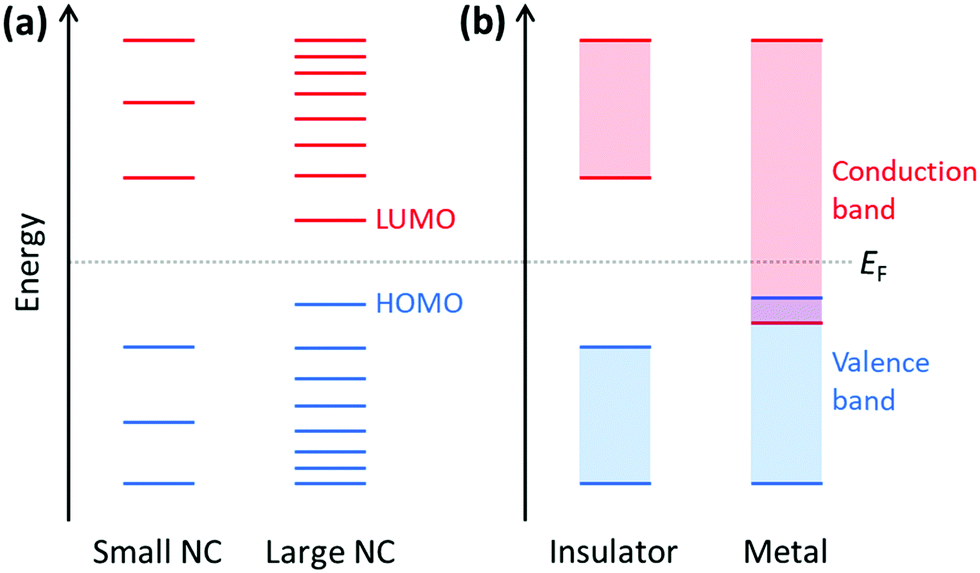 | ||
| Fig. 13 Schematic of (a) molecular orbitals in nanoclusters (NCs) and (b) band structures of insulators and metals. The Fermi level EF indicates the energy level that is 50% occupied at thermodynamic equilibrium. | ||
The main purpose of this article is to explain the distinctions between plasmonic and excitonic behavior when metal nanoclusters interact with light. Within an MO framework, when a system absorbs light, it is excited from the ground state to an excited state; any state with higher energy than the ground state is an excited state where one or more electrons are excited from occupied to unoccupied MOs. An electron configuration where one electron is excited from an occupied to an unoccupied MO is called a single (or single-particle) excitation; double, triple, or higher excitations where multiple electrons are excited are also possible. Some excited states are composed of one dominant excitation, creating an excited state that is essentially a single-particle excitation (Fig. 14a); other excited states are collective, involving a linear combination of several to many single-particle excitations (Fig. 14b). The system may also be excited vibrationally, where the excess energy increases the amplitude of the nuclear vibrational motion.
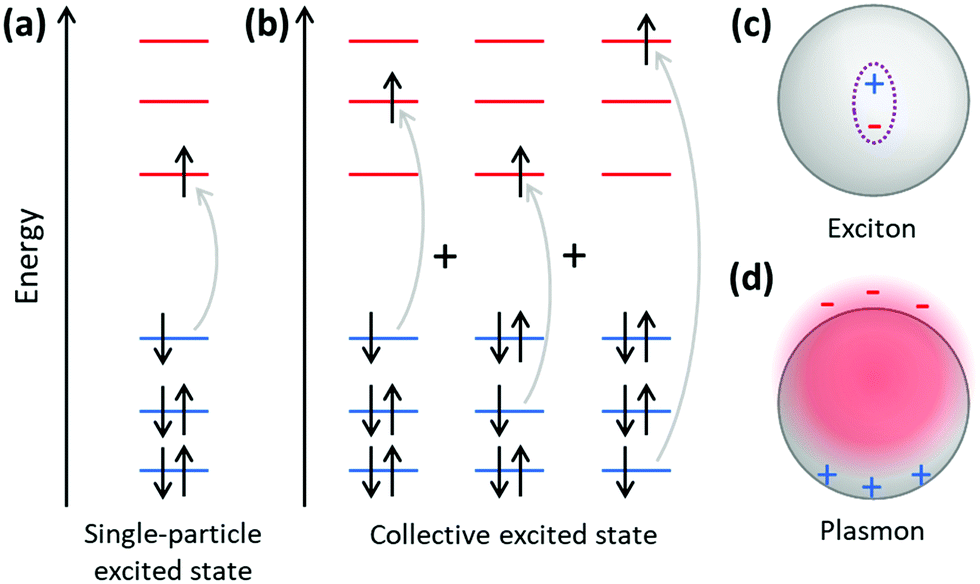 | ||
| Fig. 14 Schematic of (a) an excited state corresponding to one single-particle transition, (b) an excited state corresponding to a linear combination of several single-particle transitions, (c) an exciton, and (d) a plasmon. | ||
Within a band structure framework, when a system absorbs light, there are multiple classes of electronic excitations with different properties. A plasmon is an electronic excitation characterized by coherent oscillations of a large number of electrons (Fig. 14d), which will be discussed in much more detail in the next section; plasmons are only possible in systems that have electrons in their conduction band. In contrast, an exciton is an electronic excitation where an electron is excited from an occupied band into an unoccupied band. Because the excited electron has excess energy, it is called a hot electron; the empty energy level it leaves behind is called a hot hole. In an exciton, the negatively-charged electron and the positively-charged hole have strong enough Coulomb attractions that they are bound together (Fig. 14c). If the electrons are excited within the same band, typically within the conduction band, the excitation is termed an intraband transition; within a molecular orbital picture, excitations among the molecular orbitals that correspond to the conduction band are likewise called intraband. Conversely, if electrons are excited from one band into another band, typically from the valence band into the conduction band, the excitation is called an interband transition. We will see later that plasmons must be collective, but not all collective excited states can be classified as plasmons. In addition, phonons are collective oscillations of the nuclear motions in an extended system, analogous to vibrational excited states in molecules.
Conflicts of interest
There are no conflicts to declare.Acknowledgements
The author would like to thank Alva Dillon for providing data for the Ag8 nanowires. This work was supported by an NSF CAREER award (CHE-2046099).References
- M. Faraday, Philos. Trans. R. Soc. London, 1857, 147, 145–181 CrossRef.
- D. Bohm and D. Pines, Phys. Rev., 1951, 82, 625–634 CrossRef CAS.
- D. Pines and D. Bohm, Phys. Rev., 1952, 85, 338–353 CrossRef CAS.
- D. Bohm and D. Pines, Phys. Rev., 1953, 92, 609–625 CrossRef CAS.
- E. Ozbay, Science, 2006, 311, 189–193 CrossRef CAS.
- N. J. Halas, S. Lal, W. S. Chang, S. Link and P. Nordlander, Chem. Rev., 2011, 111, 3913–3961 CrossRef CAS.
- S. Link and M. A. El-Sayed, Int. Rev. Phys. Chem., 2000, 19, 409–453 Search PubMed.
- K. A. Willets and R. P. Van Duyne, Annu. Rev. Phys. Chem., 2007, 58, 267–297 CrossRef CAS.
- B. Sharma, R. R. Frontiera, A.-I. Henry, E. Ringe and R. P. Van Duyne, Mater. Today, 2012, 15, 16–25 CrossRef CAS.
- R. L. Gieseking, M. A. Ratner and G. C. Schatz, Frontiers of Plasmon Enhanced Spectroscopy, 2016, vol. 1, pp. 1–22 Search PubMed.
- J. Langer, D. Jimenez de Aberasturi, J. Aizpurua, R. A. Alvarez-Puebla, B. Auguié, J. J. Baumberg, G. C. Bazan, S. E. J. Bell, A. Boisen, A. G. Brolo, J. Choo, D. Cialla-May, V. Deckert, L. Fabris, K. Faulds, F. J. García de Abajo, R. Goodacre, D. Graham, A. J. Haes, C. L. Haynes, C. Huck, T. Itoh, M. Käll, J. Kneipp, N. A. Kotov, H. Kuang, E. C. L. Ru, H. K. Lee, J.-F. Li, X. Y. Ling, S. A. Maier, T. Mayerhöfer, M. Moskovits, K. Murakoshi, J.-M. Nam, S. Nie, Y. Ozaki, I. Pastoriza-Santos, J. Perez-Juste, J. Popp, A. Pucci, S. Reich, B. Ren, G. C. Schatz, T. Shegai, S. Schlücker, L.-L. Tay, K. G. Thomas, Z.-Q. Tian, R. P. Van Duyne, T. Vo-Dinh, Y. Wang, K. A. Willets, C. Xu, H. Xu, Y. Xu, Y. S. Yamamoto, B. Zhao and L. M. Liz-Marzán, ACS Nano, 2020, 14, 28–117 CrossRef CAS.
- J. N. Anker, W. P. Hall, O. Lyandres, N. C. Shah, J. Zhao and R. P. Van Duyne, Nat. Mater., 2008, 7, 442–453 CrossRef CAS.
- K. C. Bantz, A. F. Meyer, N. J. Wittenberg, H. Im, O. Kurtuluş, S. H. Lee, N. C. Lindquist, S.-H. Oh and C. L. Haynes, Phys. Chem. Chem. Phys., 2011, 13, 11551–11567 RSC.
- S. Linic, P. Christopher and D. B. Ingram, Nat. Mater., 2011, 10, 911–921 CrossRef CAS.
- W. Hou and S. B. Cronin, Adv. Funct. Mater., 2013, 23, 1612–1619 CrossRef CAS.
- J. G. Smith, J. A. Faucheaux and P. K. Jain, Nano Today, 2015, 10, 67–80 CrossRef CAS.
- M. L. Brongersma, N. J. Halas and P. Nordlander, Nat. Nanotechnol., 2015, 10, 25–34 CrossRef CAS.
- Z. Zheng, W. Xie, B. Huang and Y. Dai, Chem. – Eur. J., 2018, 24, 18322–18333 CrossRef CAS.
- M. W. Knight, N. S. King, L. Liu, H. O. Everitt, P. Nordlander and N. J. Halas, ACS Nano, 2014, 8, 834–840 CrossRef CAS.
- J. S. Biggins, S. Yazdi and E. Ringe, Nano Lett., 2018, 18, 3752–3758 CrossRef CAS.
- U. Guler, S. Suslov, A. V. Kildishev, A. Boltasseva and V. M. Shalaev, Nanophotonics, 2015, 4, 269–276 CAS.
- A. A. Barragan, S. Hanukovich, K. Bozhilov, S. S. R. K. C. Yamijala, B. M. Wong, P. Christopher and L. Mangolini, J. Phys. Chem. C, 2019, 123, 21796–21804 CrossRef CAS.
- A. Lauchner, A. E. Schlather, A. Manjavacas, Y. Cui, M. J. McClain, G. J. Stec, F. J. Garcia de Abajo, P. Nordlander and N. J. Halas, Nano Lett., 2015, 15, 6208–6214 CrossRef CAS.
- M. Jablan and D. E. Chang, Phys. Rev. Lett., 2015, 114, 1–6 CrossRef.
- T. Jensen, L. Kelly, A. Lazarides and G. C. Schatz, J. Cluster Sci., 1999, 10, 295–317 CrossRef CAS.
- K. L. Kelly, E. Coronado, L. L. Zhao and G. C. Schatz, J. Phys. Chem. B, 2003, 107, 668–677 CrossRef CAS.
- X. Kang, H. Chong and M. Zhu, Nanoscale, 2018, 10, 10758–10834 RSC.
- Y. Du, H. Sheng, D. Astruc and M. Zhu, Chem. Rev., 2020, 120, 526–622 CrossRef CAS.
- H. Qian, M. Zhu, Z. Wu and R. Jin, Acc. Chem. Res., 2012, 45, 1470–1479 CrossRef CAS.
- T. Higaki, M. Zhou, K. J. Lambright, K. Kirschbaum, M. Y. Sfeir and R. Jin, J. Am. Chem. Soc., 2018, 140, 5691–5695 CrossRef CAS.
- H. Qian, Y. Zhu and R. Jin, Proc. Natl. Acad. Sci. U. S. A., 2012, 109, 696–700 CrossRef CAS.
- R. Jin, Nanoscale, 2010, 2, 343–362 RSC.
- R. Jin, C. Zeng, M. Zhou and Y. Chen, Chem. Rev., 2016, 116, 10346–10413 CrossRef CAS.
- M. A. Abbas, P. V. Kamat and J. H. Bang, ACS Energy Lett., 2018, 3, 840–854 CrossRef CAS.
- J. Fang, B. Zhang, Q. Yao, Y. Yang, J. Xie and N. Yan, Coord. Chem. Rev., 2016, 322, 1–29 CrossRef CAS.
- M. Zhu, C. M. Aikens, F. J. Hollander, G. C. Schatz and R. Jin, J. Am. Chem. Soc., 2008, 130, 5883–5885 CrossRef CAS.
- N. Yan, N. Xia, L. Liao, M. Zhu, F. Jin, R. Jin and Z. Wu, Sci. Adv., 2018, 4, 1–8 Search PubMed.
- S. Tian, Y.-Z. Li, M.-B. Li, J. Yuan, J. Yang, Z. Wu and R. Jin, Nat. Commun., 2015, 6, 8667 CrossRef CAS.
- H. Häkkinen, Chem. Soc. Rev., 2008, 37, 1847–1859 RSC.
- H. Häkkinen, Adv. Phys.: X, 2016, 1, 467–491 Search PubMed.
- A. Muñoz-Castro, Phys. Chem. Chem. Phys., 2019, 21, 13022–13029 RSC.
- C. M. Aikens, S. Li and G. C. Schatz, J. Phys. Chem. C, 2008, 112, 11272–11279 CrossRef CAS.
- R. L. M. Gieseking, A. P. Ashwell, M. A. Ratner and G. C. Schatz, J. Phys. Chem. C, 2020, 124, 3260–3269 CrossRef CAS.
- D. Casanova, J. M. Matxain and J. M. Ugalde, J. Phys. Chem. C, 2016, 120, 12742–12750 CrossRef CAS.
- R. Zhang, L. Bursi, J. D. Cox, Y. Cui, C. M. Krauter, A. Alabastri, A. Manjavacas, A. Calzolari, S. Corni, E. Molinari, E. A. Carter, F. J. García De Abajo, H. Zhang and P. Nordlander, ACS Nano, 2017, 11, 7321–7335 CrossRef CAS.
- L. Bursi, A. Calzolari, S. Corni and E. Molinari, ACS Photonics, 2016, 3, 520–525 CrossRef CAS.
- M. M. Müller, M. Kosik, M. Pelc, G. W. Bryant, A. Ayuela, C. Rockstuhl and K. Słowik, J. Phys. Chem. C, 2020, 124, 24331–24343 CrossRef.
- C. M. Krauter, S. Bernadotte, C. R. Jacob, M. Pernpointner and A. Dreuw, J. Phys. Chem. C, 2015, 119, 24564–24573 CrossRef CAS.
- S. Bernadotte, F. Evers and C. R. Jacob, J. Phys. Chem. C, 2013, 117, 1863–1878 CrossRef CAS.
- R. Aroca, Surface-Enhanced Vibrational Spectroscopy, John Wiley & Sons, Ltd, Chichester, UK, 2006 Search PubMed.
- G. V. Hartland, Chem. Rev., 2011, 111, 3858–3887 CrossRef CAS.
- U. Kreibig and M. Vollmer, Optical Properties of Metal Clusters, Springer, New York, 1995 Search PubMed.
- P. Drude, Ann. Phys., 1900, 306, 566–613 CrossRef.
- P. Drude, Ann. Phys., 1900, 308, 369–402 CrossRef.
- R. W. Wood, Phys. Rev., 1933, 44, 353–360 CrossRef CAS.
- G. Mie, Ann. Phys., 1908, 330, 377–445 CrossRef.
- B. T. Draine and P. J. Flatau, J. Opt. Soc. Am. A, 1994, 11, 1491 CrossRef.
- E. A. Coronado and G. C. Schatz, J. Chem. Phys., 2003, 119, 3926–3934 CrossRef CAS.
- M. D. Sonntag, E. A. Pozzi, N. Jiang, M. C. Hersam and R. P. Van Duyne, J. Phys. Chem. Lett., 2011, 5, 3125–3130 CrossRef.
- N. L. Gruenke, M. F. Cardinal, M. O. McAnally, R. R. Frontiera, G. C. Schatz and R. P. Van Duyne, Chem. Soc. Rev., 2016, 45, 2263–2290 RSC.
- F. Neubrech, C. Huck, K. Weber, A. Pucci and H. Giessen, Chem. Rev., 2017, 117, 5110–5145 CrossRef CAS.
- M. Bauch, K. Toma, M. Toma, Q. Zhang and J. Dostalek, Plasmonics, 2014, 9, 781–799 CrossRef CAS.
- S. H. Yau, O. Varnavski and T. Goodson, Acc. Chem. Res., 2013, 46, 1506–1516 CrossRef CAS.
- M. Zhou and R. Jin, Annu. Rev. Phys. Chem., 2021, 72, 121–142 CrossRef CAS.
- S. Link and M. A. El-Sayed, Annu. Rev. Phys. Chem., 2003, 54, 331–366 CrossRef CAS.
- J. Olesiak-Banska, M. Waszkielewicz, P. Obstarczyk and M. Samoc, Chem. Soc. Rev., 2019, 48, 4087–4117 RSC.
- S. Link and M. A. El-Sayed, J. Phys. Chem. B, 1999, 103, 8410–8426 CrossRef CAS.
- A. Cirri, H. M. Hernández and C. J. Johnson, J. Phys. Chem. A, 2020, 124, 1467–1479 CrossRef CAS.
- R. Mittal, R. Glenn, I. Saytashev, V. V. Lozovoy and M. Dantus, J. Phys. Chem. Lett., 2015, 6, 1638–1644 CrossRef CAS.
- R. L. Olmon, B. Slovick, T. W. Johnson, D. Shelton, S.-H. Oh, G. D. Boreman and M. B. Raschke, Phys. Rev. B: Condens. Matter Mater. Phys., 2012, 86, 235147 CrossRef.
- F. Hubenthal, Plasmonics, 2013, 8, 1341–1349 CrossRef CAS.
- G. Tas and H. J. Maris, Phys. Rev. B: Condens. Matter Mater. Phys., 1994, 49, 15046–15054 CrossRef CAS.
- R. H. M. Groeneveld, R. Sprik and A. Lagendijk, Phys. Rev. B: Condens. Matter Mater. Phys., 1992, 45, 5079–5082 CrossRef.
- S. Link, C. Burda, Z. L. Wang and M. A. El-Sayed, J. Chem. Phys., 1999, 111, 1255–1264 CrossRef CAS.
- M. Bernardi, J. Mustafa, J. B. Neaton and S. G. Louie, Nat. Commun., 2015, 6, 7044 CrossRef CAS.
- V. P. Zhukov, F. Aryasetiawan, E. V. Chulkov, I. G. de Gurtubay and P. M. Echenique, Phys. Rev. B: Condens. Matter Mater. Phys., 2001, 64, 195122 CrossRef.
- M. Aeschlimann, M. Bauer, S. Pawlik, R. Knorren, G. Bouzerar and K. H. Bennemann, Appl. Phys. A: Mater. Sci. Process., 2000, 71, 485–491 CrossRef CAS.
- W. S. Fann, R. Storz, H. W. K. Tom and J. Bokor, Phys. Rev. B: Condens. Matter Mater. Phys., 1992, 46, 13592–13595 CrossRef CAS.
- E. Knoesel, A. Hotzel, T. Hertel, M. Wolf and G. Ertl, Surf. Sci., 1996, 368, 76–81 CrossRef CAS.
- N. Del Fatti, C. Voisin, M. Achermann, S. Tzortzakis, D. Christofilos and F. Vallée, Phys. Rev. B: Condens. Matter Mater. Phys., 2000, 61, 16956–16966 CrossRef CAS.
- S. I. Anisimov, B. L. Kapeliovich and T. L. Perel-man, J. Exp. Theor. Phys., 1974, 66, 375–377 Search PubMed.
- T. S. Ahmadi, S. L. Logunov and M. A. El-Sayed, J. Phys. Chem., 1996, 100, 8053–8056 CrossRef CAS.
- S. L. Logunov, T. S. Ahmadi, M. A. El-Sayed, J. T. Khoury and R. L. Whetten, J. Phys. Chem. B, 1997, 101, 3713–3719 CrossRef CAS.
- M. Zhou, C. Yao, M. Y. Sfeir, T. Higaki, Z. Wu and R. Jin, J. Phys. Chem. C, 2018, 122, 13435–13442 CrossRef CAS.
- M. S. Devadas, J. Kim, E. Sinn, D. Lee, T. Goodson and G. Ramakrishna, J. Phys. Chem. C, 2010, 114, 22417–22423 CrossRef CAS.
- T. Stoll, E. Sgrò, J. W. Jarrett, J. Réhault, A. Oriana, L. Sala, F. Branchi, G. Cerullo and K. L. Knappenberger, J. Am. Chem. Soc., 2016, 138, 1788–1791 CrossRef CAS.
- K. G. Stamplecoskie and P. V. Kamat, J. Am. Chem. Soc., 2014, 136, 11093–11099 CrossRef CAS.
- M. Zhou, S. Tian, C. Zeng, M. Y. Sfeir, Z. Wu and R. Jin, J. Phys. Chem. C, 2017, 121, 10686–10693 CrossRef CAS.
- M. Zhou, C. Zeng, M. Y. Sfeir, M. Cotlet, K. Iida, K. Nobusada and R. Jin, J. Phys. Chem. Lett., 2017, 8, 4023–4030 CrossRef CAS.
- S. H. Yau, O. Varnavski, J. D. Gilbertson, B. Chandler, G. Ramakrishna and T. Goodson, J. Phys. Chem. C, 2010, 114, 15979–15985 CrossRef CAS.
- O. P. Varnavski, T. Goodson, M. B. Mohamed and M. A. El-Sayed, Phys. Rev. B: Condens. Matter Mater. Phys., 2005, 72, 235405 CrossRef.
- S. Link, M. A. El-Sayed, T. Gregory Schaaff and R. L. Whetten, Chem. Phys. Lett., 2002, 356, 240–246 CrossRef CAS.
- H. Qian, M. Y. Sfeir and R. Jin, J. Phys. Chem. C, 2010, 114, 19935–19940 CrossRef CAS.
- T. D. Green and K. L. Knappenberger, Nanoscale, 2012, 4, 4111 RSC.
- S. Mustalahti, P. Myllyperkiö, T. Lahtinen, K. Salorinne, S. Malola, J. Koivisto, H. Häkkinen and M. Pettersson, J. Phys. Chem. C, 2014, 118, 18233–18239 CrossRef CAS.
- C. Yi, H. Zheng, L. M. Tvedte, C. J. Ackerson and K. L. Knappenberger, J. Phys. Chem. C, 2015, 119, 6307–6313 CrossRef CAS.
- R. L. Gieseking, M. A. Ratner and G. C. Schatz, J. Phys. Chem. A, 2016, 120, 4542–4549 CrossRef CAS.
- R. L. M. Gieseking, Chem. Mater., 2019, 31, 6850–6859 CrossRef CAS.
- R. L. Gieseking, M. A. Ratner and G. C. Schatz, J. Phys. Chem. A, 2016, 120, 9324–9329 CrossRef CAS.
- N. V. Ilawe, M. B. Oviedo and B. M. Wong, J. Chem. Theory Comput., 2017, 13, 3442–3454 CrossRef CAS.
- S. D’Agostino, R. Rinaldi, G. Cuniberti and F. Della Sala, J. Phys. Chem. C, 2018, 122, 19756–19766 CrossRef.
- N. Asadi-Aghbolaghi, R. Rüger, Z. Jamshidi and L. Visscher, J. Phys. Chem. C, 2020, 124, 7946–7955 CrossRef CAS.
- Z. Liu, F. Alkan and C. M. Aikens, J. Chem. Phys., 2020, 153, 144711 CrossRef CAS.
- E. Townsend and G. W. Bryant, J. Opt., 2014, 16(11), 114022 CrossRef.
- E. Selenius, S. Malola and H. Häkkinen, J. Phys. Chem. C, 2017, 121, 27036–27052 CrossRef CAS.
- J. Ma, Z. Wang and L.-W. Wang, Nat. Commun., 2015, 6, 10107 CrossRef CAS.
- F. Ding, E. B. Guidez, C. M. Aikens and X. Li, J. Chem. Phys., 2014, 140, 244705 CrossRef.
- G. U. Kuda-Singappulige, D. B. Lingerfelt, X. Li and C. M. Aikens, J. Phys. Chem. C, 2020, 124, 20477–20487 CrossRef CAS.
- O. Ranasingha, H. Wang, V. Zobač, P. Jelínek, G. Panapitiya, A. J. Neukirch, O. V. Prezhdo, J. P. Lewis, P. Jelinek, G. Panapitiya, A. J. Neukirch, O. V. Prezhdo and J. P. Lewis, J. Phys. Chem. Lett., 2016, 7, 1563–1569 CrossRef CAS.
- R. D. Senanayake, A. V. Akimov and C. M. Aikens, J. Phys. Chem. C, 2017, 121, 10653–10662 CrossRef CAS.
- S. L. Brown, E. K. Hobbie, S. Tretiak and D. S. Kilin, J. Phys. Chem. C, 2017, 121, 23875–23885 CrossRef CAS.
- E. Townsend and G. W. Bryant, Nano Lett., 2012, 12, 429–434 CrossRef CAS.
- L. Bursi, A. Calzolari, S. Corni and E. Molinari, ACS Photonics, 2014, 1, 1049–1058 CrossRef CAS.
- M. Walter, J. Akola, O. Lopez-Acevedo, P. D. Jadzinsky, G. Calero, C. J. Ackerson, R. L. Whetten, H. Gronbeck and H. Hakkinen, Proc. Natl. Acad. Sci. U. S. A., 2008, 105, 9157–9162 CrossRef CAS.
- M. Zhu, C. M. Aikens, M. P. Hendrich, R. Gupta, H. Qian, G. C. Schatz and R. Jin, J. Am. Chem. Soc., 2009, 131, 2490–2492 CrossRef CAS.
- D. E. Jiang, M. Kühn, Q. Tang and F. Weigend, J. Phys. Chem. Lett., 2014, 5, 3286–3289 CrossRef CAS.
- P. N. Day, R. Pachter, K. A. Nguyen and R. Jin, J. Phys. Chem. A, 2019, 123, 6472–6481 CrossRef CAS.
- S. Takano, S. Yamazoe and T. Tsukuda, APL Mater., 2017, 5, 3–8 Search PubMed.
- A. P. Ashwell, M. A. Ratner and G. C. Schatz, in Advances in Quantum Chemistry, ed. J. R. Sabin and E. J. Brändas, Academic Press, Cambridge, MA, 2017, vol. 75, pp. 117–145 Search PubMed.
- E. B. Guidez and C. M. Aikens, Phys. Chem. Chem. Phys., 2014, 16, 15501–15509 RSC.
- S. Malola, L. Lehtovaara, J. Enkovaara and H. Häkkinen, ACS Nano, 2013, 7, 10263–10270 CrossRef CAS.
- T. P. Rossi, M. Kuisma, M. J. Puska, R. M. Nieminen and P. Erhart, J. Chem. Theory Comput., 2017, 13, 4779–4790 CrossRef CAS.
- J. Yan and S. Gao, Phys. Rev. B: Condens. Matter Mater. Phys., 2008, 78, 235413 CrossRef.
- B. Gao, K. Ruud and Y. Luo, J. Chem. Phys., 2012, 137, 194307 CrossRef.
| This journal is © The Royal Society of Chemistry 2022 |