Complex amorphous oxides: property prediction from high throughput DFT and AI for new material search

Abstract

With decreasing dimensions and increasing complexity, semiconductor devices are getting more difficult to fabricate. In particular the allowed deposition temperature becomes lower. Amorphous materials, which do not require annealing steps, are therefore becoming more interesting. First principles modelling of amorphous materials is, however, way more complex than modelling crystalline ones. Especially to screen for new materials, a fully ab initio approach is hence too expensive. We take on this challenge by employing a combination of high throughput first principles calculations and artificial intelligence (AI). We construct 4500 atomistic models, each containing 200-atoms, to capture the properties of amorphous phases of primary, X–O, and binary, X–Y–O, metal oxides. For these models, we calculate the relevant properties for a transistor channel. Expanding this exercise to more complex metal oxides would lead to a prohibitively large number of options. We solve this problem by training support vector regression models based on the data generated for the primary and binary oxides to predict the properties of ternary and more complex oxides. By combining the trained models, we construct an objective function that, at its minimum, points to the optimal composition in terms of electronic performances and material stability. After screening a series of objective functions, we identify the Zn–Mg–Al–O metal oxide (Zn and Mg around 40–50 at%, Al below 10 at%) as being the most interesting improvement to the current industry standard a-IGZO for the development of a high charge carrier mobility layer of a thin film transistor compatible with low deposition temperature requirements. It is predicted to combine an improvement in terms of electron mobility and chemical stability with respect to a-IGZO. This method, combining first principles calculated data with AI, is however not restricted to finding new materials for the active layer in a thin film transistor. From a general perspective, this approach can be used for any alloy or compound discovery problem, in which the pivotal material properties can be calculated for, in the order of a thousand, relevant one- and two-element materials.

---

1 Introduction

Since the first signs of a slowing down of Morses law in the traditional area scaling of semiconductor devices, the industry has been turning its interest to new device architectures. The combination of new architectures with the advancements in extreme ultraviolet lithography technologies is predicted to sustain the down-scaling for probably another decade. The performance increase at fixed power, however, does seem to be coming to a halt when continuing with standard materials like silicon. On top of this, the combination of high mobility van der Waals materials with three-dimensional CMOS architectures is under development, requiring more heterogeneous integration schemes. One thing that all these developments have in common is the need for new materials with a low deposition temperature to be co-integrated on a silicon platform.

Amorphous materials, in general, allow for lower deposition temperatures than crystalline ones, enabling more complex CMOS device structures and the fabrication of large area transistors on non-silicon based substrates such as plastic.^1,2 They, therefore, can provide a viable option for the active layer of thin film transistors in these demanding new architectures, provided that they show electrical performances similar to crystalline silicon. Unfortunately, upon amorphization, most materials suffer from a significant reduction of their charge carrier mobilities, making them useless for high performance computing applications. Interestingly, amorphous metal oxides tend to have a higher mobility than amorphous silicon.³

Probably the best-known demonstration of a successful amorphous oxide is the introduction of InGaZnO₄ (IGZO) as a transistor channel material. IGZO found its application first in thin-film-transistor (TFT) display backplanes,^4–9 and more recently as a transistor channel material for static random access memory (SRAM)¹⁰ or as a memory selector in dynamic random access memory (DRAM) devices.^9,11–15 However, introducing amorphous oxides as transistor channels requires gaining a tight control on the different doping sources to ensure appropriate device operation and a low access contact resistance. In particular, the electron mobility and chemical stability of IGZO are far from being ideal, with a high sensitivity to hydrogen inclusion and oxygen depletion sources,^3,16–21 leading to complex integration schemes.

Many attempts have been made to identify ‘material(s) beyond IGZO’ that would solve these issues, and reports on high mobility amorphous oxides are numerous but also often contradictory, see Fig. 1. Part of the problem comes from the difficulty to extract non-ambiguous charge carrier mobilities. Until recently, numerous primary and binary oxides were reported to display mobilities reaching sometimes well over 200 cm² V⁻¹ s⁻¹.^22–36

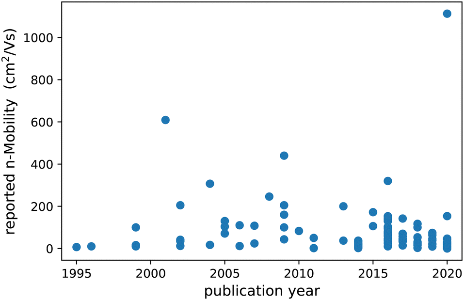Fig. 1 Reported mobility of n-type channel materials over the years.

In the second half of the last decade, many more promising new amorphous oxides were reported. Compared to earlier works, the composition of the materials became more complex, and mainly ternary oxides were reported on.^37–63 The extreme super high mobilities reported in previous studies, i.e. above 100 cm² V⁻¹ s⁻¹, were however not seen anymore, except for some outliers.

Finally, in the 2020s, the reported materials become more and more complex with quaternary oxides becoming more common than before.^64–71 A few exceptions excluded, most reported mobilities are now all below 50 cm² V⁻¹ s⁻¹. One would almost be tempted to start believing that electron mobility in complex oxides is a time dependent property.

Although many materials have hence been reported, some with very promising properties, IGZO is currently still the only one making its way into actual devices. The search for new materials is hence still a very active field. However, due to the combinatorial explosion of options, when more and more elements per material are considered, a systematic search in a composition space this large is more like finding missing luggage in Hilberts hotel than looking for the proverbial needle in a haystack.

Comparing all reported mobilities, even on identical materials, moreover, often shows large variations, sometimes by orders of magnitude. This suggests that quantifying key parameters like mobility, in a transparent and comparable way is not an easy task. Consequently, comprehensive studies aiming at the discovery of trends and material design guidelines are limited.^47,72–74

Fortunately, in recent years, a new approach has been emerging to address such challenges. By collecting large amounts of structural and electronic properties, either being calculated or experimentally obtained, and combining these with machine learning, new materials and the mapping of known materials to new applications are being discovered.^75–93 Most of these works, however, mainly focused on crystalline materials and around variations of elements and sites in known crystalline materials. Although systems of off-stoichiometic compositions and materials of unknown structure are also getting attention,^94,95 the use of amorphous materials, which is the focus of our interest, adds even more additional difficulties.

In this work, we address this challenge by combining density functional theory (DFT) calculations with machine learning. For a set of elements, see Fig. 2, selected from the different candidates reported in the literature, we collect known crystalline phases of all primary, single element, and binary, two element oxides. From the structural properties of these crystalline phases, we create primary and binary amorphous models. For the amorphous models, we calculate the key electronic and chemical properties, which are then used to train machine learning models to predict them for any arbitrary complex amorphous oxide. Finally, we minimise an objective function containing all these models to predict interesting new candidates, offering the best trade-off in terms of electronic properties and stability. For the most promising candidates, we validate the machine learning model prediction by explicit DFT calculations.

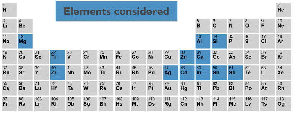Fig. 2 The 12 elements for which the amorphous oxides and combinations of them are considered in this study.

2 Methodology

2.1 Overall Workflow

The overall workflow in this study follows the five steps described below. Further explicit details are provided in the next subsections.

Collect known crystals. We start by collecting known crystalline phases of primary and binary oxides of 12 selected elements. We selected the representative elements found in the n-type channel materials reported in the literature so far, see the discussion in the Introduction section. The Materials Project database⁹⁶ is used for this purpose. We analyse the structural features of the crystalline phases to extract the local geometries and building motives and use these to build amorphous atomistic models for known and hypothetical metal(loid) ratios. We select stable phases of the composition having the largest band gap in case of multiple options. Using these ratios is then expected to also lead to large gaps in the amorphous phases. By selecting the most stable phases we attempt to extract the most stable local motives which should also dominate the amorphous structures.

Construct amorphous models for primary and binary systems. We include (close to) 1 : 20, 1 : 10, and 1 : 5 ratios of the elements besides the known ratios, which are often close to 1 : 1 or 1 : 2. The amount of oxygen is always set at the stoichiometric amount. The amorphous models are then structurally optimised using density functional theory calculations. After the structural optimisation step, the observables, total energy and electronic properties, are calculated and collected.

Train models to reproduce primary and binary systems and predict more complex systems. The primary and binary oxides form the 2D boundary of a 11D elemental space. A full systematic screening of the insides with explicit calculations on atomistic models is practically impossible. We therefore train support vector regression models (SVR) on the computed observables to predict the properties of the complex materials inside this space. We use a feature vector containing only the composition of the material to develop the models.

Define and optimise an objective function. To find new material classes, we combine the different regression models into a single objective function. This function is constructed such that moving toward an optimal value of each of the individual contributions reduces its value. Overall minimisation of the function hence leads to candidate materials where the different properties are optimal.

Validation. Finally, for the most interesting resulting material classes, we validate the model predictions by explicit calculations. We generate new atomistic amorphous models of the predicted compositions, calculate their properties, and compare them to the model predictions.

2.2 First principles calculations of the observables

All first principles calculations reported in this paper, are performed in the framework of Kohn–Sham Density Functional Theory^97–99 (DFT) using the CP2K software package.¹⁰⁰ The hybrid Gaussian and plane wave density functional scheme of CP2K^101–105 ensure that the dimension of the systems, needed to reach low concentrations of defects, are computationally feasible. We used the PBEsol generalised gradient approximation for the exchange correlation functional.^106,107 The standard DZVP basis sets¹⁰⁸ and pseudo potentials^109–111 provided with CP2K are used. Given the amorphous phase of the materials, all calculations are performed using the Γ–point only. For the structure optimisation, we use a maximum geometry change convergence criterion of 5 mBohr and a force convergence criterion of 1 mH Bohr⁻¹. The preparation, execution, monitoring, and post-processing of the over 10 000 calculations reported in this work have been facilitated by our in-house python package.

The amorphous phase is modelled in periodic unit cells containing close to 100, 200, and 400 atoms for the known composition models. For the hypothetical ratio models, we simulate only 200 atom models. For each model, we pertain strict oxygen stoichiometry since missing oxygen, in most of these materials, tends to dope it to n-type. For the hypothetical ratio models, the oxygen stoichiometry of the primary oxides is maintained per element. For each system, we generate 10 different morphologies to obtain a statistical sampling of the structure. The atomistic models for the amorphous phase have been generated by using the approach proposed by Drabold et al.,¹¹² in which a starting prototypical atomic structure is built from a random distribution of metal atoms, the atomic position is then compacted and decorated by oxygen atoms to obtain coordination numbers and bond distances typically met in crystalline phases. The resulting models are then structurally optimised using DFT. We previously used this approach to study IGZO and observed that it leads to physically sound structural models with the correct coordination number, radial distribution function, and band gap.^19,113

The mobility of electrons and holes in the amorphous phase can be hard to evaluate from first principles. For crystalline materials, where the Bloch theorem holds, a band structure can be calculated from which the curvature of the band extremes can be turned into electron and hole effective masses. For amorphous materials, this approach does not hold since translational symmetry is broken, and the Bloch theorem is not applicable anymore. In this work, we use the Inverse State Weighted Overlap (ISWO) as a measure for electron and hole mobility to capture both the degree of delocalization of the electronic states and their spatial connectivity.¹¹⁴ The ISWO value is constructed such that it behaves like an effective mass. A low value means a large electronic and spatial overlap, allowing easy carrier hopping and hence good mobility. In the present work, we look for an n-type channel material. Devices made of it should have a high on and low off current. The conduction ISWO, ISWO_C, should be as low as possible and the valence ISWO, ISWO_V, should be as high as possible to achieve this. We stress that the ISWO only provides a qualitative way to rank materials in terms of electron and hole mobility. It is in no way directly related to mobility. In previous work it has been tested systematically for various types of test systems and has be found to outperform comparable methods like the inverse participation ratio method.¹¹⁴

Evaluating the ISWO for an individual state is a clear procedure. However, defining the average ISWO of the bottom of the conduction and of the top of the valence bands in an automated manner, as we need here, is a more complex issue. The difficulty arises from the amorphous nature of the system which often leads to the occurrence of localised tail states,^{17,18,115,116} which need to be detected and excluded in the evaluation of the band gap and the ISWOs. These tail states arise from suboptimal local structural atomic arrangements. They are more localised than the actual band edges and show in the density of states at densities too low to contribute significantly to the conduction. The localisation can, however, still be on a length-scale larger than the unit cells used which makes it not a very useful criterion in high-throughput work. Too large unit cells would be needed to unambiguously detect them based on a localisation criterion. The density of states, on the other hand, can be used. For a single material, one can inspect the distribution of the ISWO vs. state energy to identify tail states. In the high-throughput situation of the present project, the individual inspection of each system is impossible. For identifying the tail states based on the density of states, we adopt the following procedure. We first calculate the average level spacing of the last 20 occupied and first 20 unoccupied electronic states. The top occupied states that are more than 2 times the average level spacing removed from other occupied states are considered tail states. In a similar manner, we remove the tail states close to the conduction band. In most of the cases, we end up identifying on average 2.3 conduction and 2.8 valence tail states per system. Finally, after the tail states are excluded, we calculate the average ISWO in a window of 0.3 eV adjacent to the band edges.

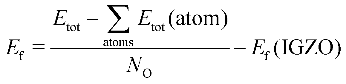
The chemical stability of the oxides is measured as the formation energy computed at 0 K from the isolated gas phase atoms. We re-scale the energy by the number of oxygen atoms and take it relative to IGZO, calculated according to the same procedure.

where E_tot is the electronic total energy computed with the PBEsol functional, and N_O is the number of oxygen atoms. Negative values, hence, point to materials more stable than IGZO. This definition allows us to identify whether a system is thermodynamically stable against typical issues met in nano-electronic integration steps, such an oxygen scavenging induced by contacting certain metals or against a reduction upon hydrogen annealing.¹¹³

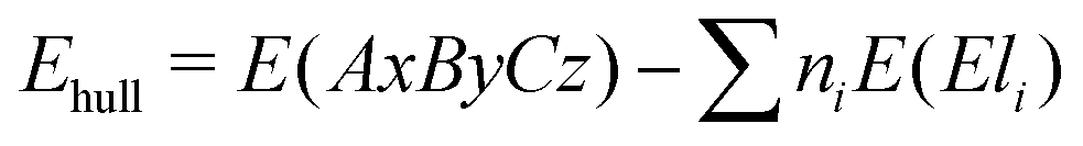
Using the formation energy as described above, we can also assess the stability of new materials against de-mixing. By using the formation energies of the constituting primary oxides, the stability of a new candidate against the decomposition into elemental amorphous phases can be assessed using the expression:

which is similar to the convex hull energy evaluation often used for solids, with the difference that the hull is planar since we do not add any elemental compounds to the hull. E_hull is not included in our objective function but rather used for our most interesting candidates. This provides some handle on how likely it would be to actually deposit the materials in the intended mixed amorphous form.

2.3 Machine learning

Selecting the feature vector for the models to work with is one of the most important steps in developing a useful predictive model. Recent work by Liu et al.⁸⁷ discusses this point in detail in the context of material properties prediction. In the present problem we ultimately need to search for new compositions. We, hence, only have access to a normalised composition vector. If we were to add features beyond the composition, we would need to somehow obtain them from structural models which, by design, we do not have available. From the composition vector, we also exclude the explicit oxygen concentration. For all non-oxygen elements, the corresponding amount of oxygen is kept fixed. The amount of oxygen is hence just a linear combination of the other elements. With this feature vector design we make the assumption that there is a one to one relationship between the composition and amorphous structure. Different deposition methods and conditions can lead to different amorphous phases. Including this in the modelling requires information that is very difficult to generate and include.

Based on the initial results for the known binary and primary systems, we conclude that 200 atom cells are large enough to obtain converged electronic results. The second series of binaries, those with hypothetical 1 : 20 to 1 : 5 element ratios, are hence only calculated in 200 atom systems. For each calculated composition, 10 different atomic models have been generated. From these, the 3 lowest in total energy after relaxation enter the training set.

Choosing the machine learning model useful for our data is a rather delicate problem. Linear models definitively do not have sufficient flexibility to provide useful predictions. On the other hand, Gaussian process regression also proved to be difficult due to our relatively small data set, with respect to the dimensions explored. We observed that Gaussian process regression tended to lead to over-fitting of our data and that our dataset is just not sufficiently large to use more sophisticated deep learning approaches. We achieved the most stable results using support vector regression.¹¹⁷

The machine learning is performed using the scikit-learn python package.¹¹⁸ We use a polynomial kernel of maximal degree 10 for the support vector machines. The regularisation parameter of 400 is used with an epsilon parameter of 0.001. These hyper parameters were selected based on the behaviour of the fitted function on the two element composition lines.

We validate the models in two steps. In the first instance we perform a leave one out cross validation on all pairs of elements. Here we remove in each case the three data points of a single composition. Secondly, we tested the trained model results for the made predictions. We reconstructed new atomistic models and explicitly calculated their properties and compared them to the machine learning predictions.

2.4 Predicting optima

Once the support vector models are generated, we have four trained models for quantities that need to be optimised simultaneously, namely G(x), ISWO_V(x), ISWO_C(x), and E_f(x), for the bandgap, valence and conduction ISWO, and formation energy, respectively. Using these we construct a target function F(x), which, when minimised, provides optimal compositions.

F(x) = (G(x) − G_t)² − AISWO_V(x) + BISWO_C(x) + CE_f(x) (3)

In eqn (3)x is a composition vector containing the relative amounts of the metal and metalloid elements shown in Fig. 2, A, B, and C are positive constants, and G_t is the gap target.

Choosing the target value for the gap G_t is another delicate issue. On one hand, a large band gap can be beneficial to help decrease the leakage current in transistors. However, if the gap gets too large, the material may not even act as a semiconductor and abnormally large operating voltages will be needed to manipulate the charge carriers, leading to non-switching transistors. The actual value that can be used also depends on the band alignments with the contact metals and gate dielectrics. In our search, we therefore scan over a range of target band gap values; 0, 0.25, 0.5, 0.75, and 1 eV larger than that of IGZO. In DFT@PBEsol, the bandgap of a-IGZO is 2.2 eV, Which underestimates the experimental value of 3.0–3.6^33,119,120 as can be expected semi-local DFT. Since the bandgap is large enough to always be qualitatively correct. Moreover, in this case we are interested in comparing gaps between rather similar materials; all are metal oxides. This will even enhance the expected error cancellation. In principle gaps could be calculated by more accurate methods like GW¹²¹ but despite rigorous code optimisation, bench-marking, and attempts to automation, these are still too expensive and cumbersome for projects like this.¹²²

The objective function is minimised using sequential least squares programming,¹²³ as implemented in SciPy.^124,125 To prevent being trapped in a local minimum, we restart the minimum search from 50 randomly chosen starting points per combination of objective function parameters.

3 Results

3.1 Learning from the known metal ratio calculations

Since we started our generation of the amorphous models by collecting structural features from experimentally known crystalline phases, we have all the data required to compare their properties. In crystalline phases and when there is a similarity between the oxides, one often observes a correlation between the electronic gap and the electron effective mass. In many crystalline oxides such as the spinel structures, the conduction band minimum occurs at gamma.⁹⁶ If, by changing the elemental composition, this minimum comes down in energy, the band structure curvature increases as well, leading to a negative correlation between the gap and effective mass. Looking at our results for amorphous materials, we observe that this correlation is not present anymore.

3.2 Training set

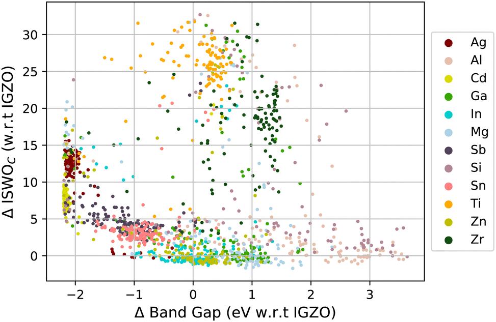
The computed results on all amorphous X–O and X–Y–O models are visualised in Fig. 3 and 4. Fig. 3 shows the ISWO value for the conduction states on the y-axis and the gap on the x-axis. All values in these plots are given relative to the average values calculated for IGZO for an easier comparison. The colour code indicates the chemical stability.

Fig. 3 Data points serving as the training set, on the x-axis the PBEsol band gap relative to that of IGZO, on the y-axis the ISWO value of the conduction states relative to that of IGZO. The colour code represents the formation energy from gas phase atoms per oxygen atom relative to the value of IGZO.

Fig. 4 The same data points as represented in Fig. 3 but with the colour map indicating the most abundant metal species.

Fig. 4 displays the same information but coloured based on the dominant element used in each material.

Before moving to the training of the machine learning models and making predictions, it is interesting to review the correlations between the material composition and the targeted properties. A direct correlation of properties with the element count on the full data set is non-conclusive. The main reason being that for any composition, the number of samples with zero content of an element is much larger than the number of samples with a finite amount of it. Moreover, the correlation between a property in the X–Y–O and the X–Z–O oxides may be more influenced by the difference between Y and Z than by the amount of X. Thereby, obscuring the effect of changing the concentration of X. We hence take all pairs of elements and calculate the correlation in the two-element space to finally take the average per element. The results are presented in Table 1.

Table 1 Correlation of features with element content. E_f denotes the formation energy, ISWO_C and ISWO_V the conduction and valence ISWO respectively, E_gap the gap, E_hull the demixing stability, and nT_C and nT_V the number of conduction and valence tail states

Elem.	E f	ISWOC	ISWOV	E gap	E hull	nT C	nT V
Zr	−0.98	0.74	0.44	0.37	−0.06	0.21	0.12
Ti	−0.75	0.65	0.19	0.07	0.07	0.06	0.19
Al	−0.59	−0.18	0.23	0.65	0.18	0.21	−0.06
Si	−0.40	−0.03	−0.14	0.81	0.28	0.55	0.37
Mg	−0.21	−0.41	0.80	0.27	0.09	0.08	−0.02
Sn	−0.03	−0.14	−0.32	−0.36	−0.09	0.10	0.04
Ga	0.04	−0.29	−0.06	0.30	−0.11	−0.05	0.24
In	0.34	−0.58	0.48	−0.16	0.05	−0.08	0.15
Zn	0.43	−0.51	−0.34	−0.11	0.15	−0.09	−0.15
Sb	0.47	0.11	−0.49	−0.37	−0.35	−0.18	0.11
Ag	0.73	0.37	−0.13	−0.61	−0.36	−0.19	−0.39
Cd	0.96	0.28	−0.69	−0.85	0.16	−0.62	−0.61

---

The strongest correlations are observed for E_f. The simulations suggest that adding Zr or Ti improves the oxide stability, while adding Ag or Cd decreases it. For the conduction ISWO, Zr, and Ti correlate strongly, with a reduction of the delocalization of the electronic states and an enhancement of the spatial spacing of the electronic states, suggesting a decrease in mobility. On the contrary, In, Zn, and Mg lead to an ISWO reduction, and point towards an increase in mobility. For E_gap Al and Si correlate positively and Ag and Cd correlate negatively. We, hence, see an inverted correlation between E_gap and E_f, i.e. that an improvement in stability always comes at the expense of an increase in band gaps. We also observe that the Ag and Sn fractions correlate negatively with E_hull. This indicates that increasing the amount of these elements reduced the tendency of phase segregation. Si behaves the other way around.

Finally, we observe an interesting relationship between the correlations: the elements that “destabilise” the formation enthalpy of the oxide, i.e., correlate positively with E_f, are associated to a lowering in the number of gap states, i.e., correlate negatively with nT_C, and in a lesser amount with nT_V. In other words, elements that decrease the chemical stability also decrease the number of intrinsic defects present in the material.

3.3 Training results

Training a model that can be used in an objective function to be minimised requires them to be relatively stiff. Models that provide too much freedom will at some point contain artificial extremes caused by over-fitting. These become clear by inspecting the resulting functions on two element composition lines, where the training set data points can be found. A global minimisation will tend to identify these and lead to incorrect results. In our exploration of the most suited machine learning models, we found that support vector regression models fit this requirement best for the present data set.

Another difficulty is that our training data set is complex. The amorphous structures force us to add multiple structural models of each composition. Since the composition is our descriptor for the models, we always end up having multiple result values per descriptor value. Since, for each composition the models can only predict one value, this leads to horizontal stripes in the plots in Fig. 5. In optimising the hyper parameters of the models, we also tuned the number of included systems per composition. Our main motivation in this process was to obtain a predictive power as high as possible, i.e. the smallest prediction errors, while obtaining models that do not contain artificial extremes from over fitting. This process was guided by comparing the fitted models to the actual data on the two element 1D sub-spaces. These plots are available interactively in the supplementary material. In this process it turned out that keeping the three most stable structural models per composition leads to slightly more predictive and stable models than keeping only single average or median values. Keeping more than three led for some parts of the data to less useful models, mainly by leading to over-fitting.

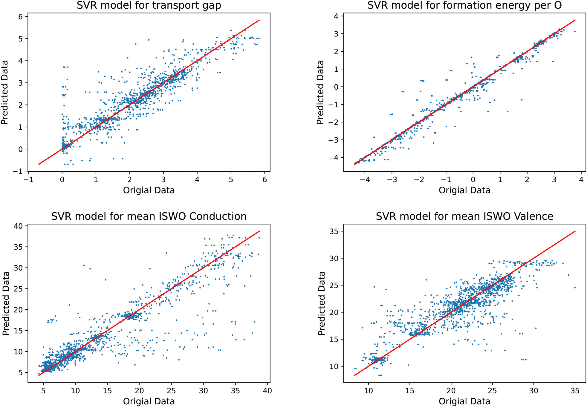Fig. 5 Results of the trained models compared to the original data for the gap (top left), formation energy (top right), ISWO Conduction (bottom left), and ISWO Valence (bottom right).

A numerical evaluation of the performance of the SVR models on the full data is shown in Fig. 5 and is listed in Table 2. Both the table and the figure indicate that E_f is the easiest to be captured by the machine learning model thanks to the global and averaged nature of the binding energies defining the enthalpy of the formation of the oxides. The occurrence of a single bond being under stress somewhere in the model has a minor impact on the total energy per atom. However, features like the gap and ISWOs are quite different. Although we automatically reject obvious tail states, the actual band gap value is still determined by the difference in energy between two states, which are very sensitive to variations in the atomic coordination.

Table 2 Quality of fit quantifiers for the obtained models

Model	Mean absolute deviation	R ^2	Pearson correlation
E gap	0.30	0.86	0.93
ISWOV	1.65	0.74	0.86
ISWOC	1.90	0.82	0.91
E f	0.16	0.96	0.98

---

In predictions for the ISWO and gap values we observe several severe outliers. These points do not show any correlation. There are only some individual systems that have serious outlier errors for two observables at the same time. These cases, however, do not form a specific class of materials.

To assess the predictive power of the models we also perform a leave one composition out cross validation on all pairs of elements. For each pair, we train the four models on training sets with the three data points for one composition removed. We then predict the values for the removed composition and calculate the mean absolute deviation (MAD). These are then averaged per left out composition and finally over all pairs.

Overall, we observe that the MAD calculated in this leave one composition out cross-validation scheme as reported in Table 3 does not deviate much from those calculated for the full set in Table 2.

Table 3 Statistics on the leave one out cross validation. The mean absolute deviation between the prediction and the actual value for a composition is calculated when the models have been calculated without that composition

	E gap	E f	ISWOV	ISWOC
Mean	0.44	0.29	2.13	2.19
Std	0.22	0.28	1.73	1.18
Min	0.05	0.04	0.42	0.83
25%	0.31	0.08	0.93	1.39
50%	0.39	0.17	1.48	1.86
75%	0.51	0.45	2.64	2.74
Max	1.33	1.25	6.74	6.24

---

3.4 Prediction

3.4.1 Predictions on the full elemental space. Choosing a series of band gap targets combined with a matrix for the relative weights A, B, and C for eqn (3) leads to a long list of predicted ternary and quaternary candidates. We use gap target values of 0, 0.25, 0.5, 0.75, and 0.1 beyond the gap of IGZO. A is varied between 0.01 and 0.02, B is varied between 0.1, 0.2, and C is varied between 0.0, 0.5, 1.0, and 1.5. Due to the complexity of the 11D elemental space, we review them based on the expected increase change in band gap with respect to a-IGZO.

Walking through the results from the smallest to the largest gaps, the first material to appear as a prediction is InO. This is completely in line with expectations. Crystalline In–O is reported to be among the oxides with the highest electron mobilities.^126–128 The models also predict the dilemma of In–O; namely, its stability (about 0.2 eV per O less stable than a-IGZO). It is not reductive enough to retain oxygen. Upon exposure to a reducing ambient (such as a hydrogen forming gas annealing step or in contact with a more reducing metal), it will release oxygen, which dopes the material n-type. Its use as a channel material in a TFT is therefore compromised since a large negative gate voltage would be needed to manipulate the charge carriers and switch the transistor off.

The next class of materials encountered is stabilised In–O with Ga and Al. As the predicted gaps steadily approach that of IGZO, so does the stability. In this class of materials, no significant stabilisation beyond IGZO is achieved. The mobility on the other hand is predicted to be improved for materials that can be classified as In rich IGZO.

From gaps of 0.3 larger than a-IGZO onwards, we encounter a new class of materials, Mg–Zn–Al where the Mg–Zn ratio ranges from 5 : 6 to 7 : 4 and the aluminium content ranges from 0 to 15 at%. This class of materials is also the most interesting result appearing from our study. Fig. 6 provides details of the four properties entering the objective function and the roles of the three elements become immediately clear. Increasing the amount of Al increases both the gap and the stability of the material. This is a general correlation in our dataset bound to the ionic nature of the alloys. The amplitude of the charge transfer in the X–O bonds increases both the band gap and the stability. In terms of conduction band ISWO, we observe a minimum along the Zn–Mg composition line (i.e. a maximised electron conductivity), which qualitatively corresponds with the phase transition from the hexagonal, at low Mg content, to cubic at high Mg content for crystalline Mg–Zn–O.¹²⁹

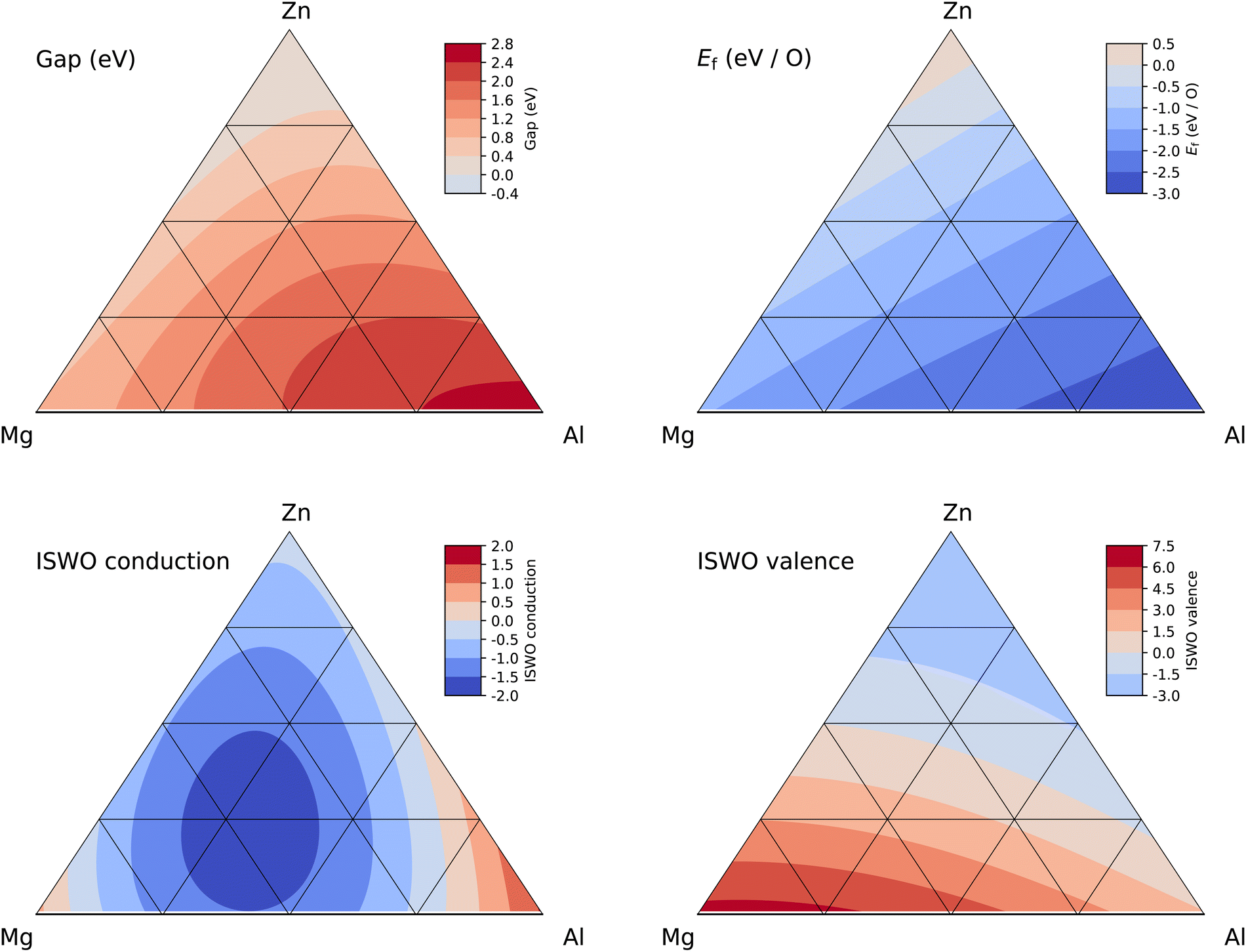Fig. 6 Ternary diagrams of gap (top left), E_f (top right), ISWO conduction (bottom left), and ISWO valence (bottom right) for the Zn–Mg–Al amorphous oxide system.

Along the Mg–Al and Zn–Al composition lines, we also observe a minimum in the conduction band ISWO. The SVR model hence predicts an overall minimum in the middle of the quaternary oxide diagram. However, moving to this minimum leads to an enhancement of the band gap setting the material composition to the insulator categories, from which no switchable transistors can be made. From a hole mobility perspective, the SVR model predicts no significant change in the ISWO_V, between the different Zn, Mg, and Al ratios. This is consistent with the composition of the valence band structure which is composed by the signature of the free electron pair of the oxygen atoms. The ultimate optimal composition is hard to predict however, since it all depends on the allowed band gap size, which in turn is dictated by the band alignment in a specific device architecture.

In terms of materials growth, it is important to establish to what extent the predicted element ratios need to be achieved exactly, which is reflected by cross-sections of the diagrams in Fig. 6 (see Fig. 7). From this representation, we can estimate the stability of the computed properties as a function of the composition.

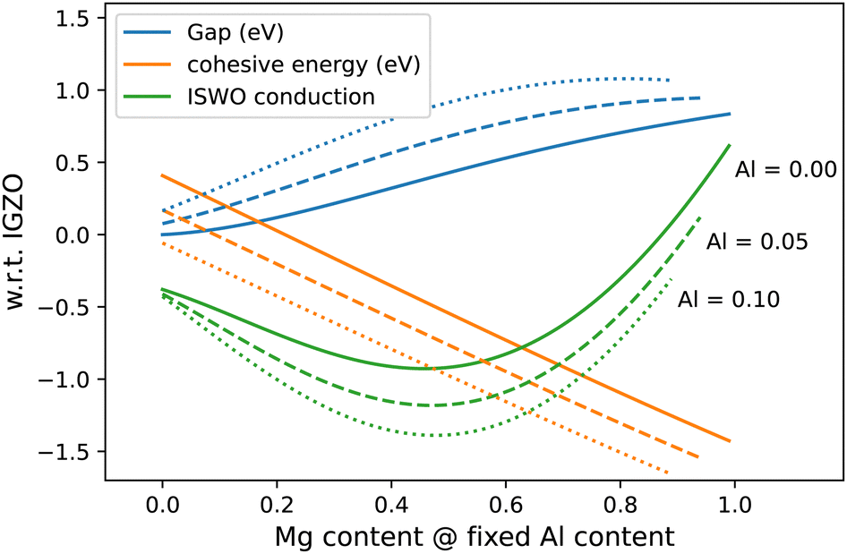Fig. 7 Cuts through the gap, formation energy, and ISWO conduction diagram for varying Mg : Zn ratio for three fixed Al concentrations.

In Fig. 7 we observe that, near the optimal region (Mg : Zn 1 : 1 and [Al] 5–10 at%) the properties are twice as sensitive to the Al concentration than to the ratio between Mg and Zn. In general, we conclude that during the deposition process, a composition error of up to 10% in the Mg : Zn ratio is acceptable but that an error of about 5% in the Al content can start to be problematic.

3.4.2 Predictions on reduced elemental spaces. Predicting new candidates based on calculated properties unfortunately does not ensure that they can be deposited. The tuning of the film growth based on either an atomic layer deposition (ALD), or on a physical vapour deposition (PVD) process may be very hard if, for instance, the sputtering rates of the different element targets are very different. On top of this, some compositions may undergo some phase segregation or partially crystallise, leading to complex heterogeneous materials. To anticipate this eventuality, we also minimise our objective function in some reduced elemental spaces to identify the “best-in-class” solutions. To increase the chance of predicting only materials that can actually be produced, we filter these results on E_hull, see eqn (2). Only those predictions that do not have an intrinsic tendency to phase segregate into single element amorphous phases are kept.
3.4.2.1 In excluded predictions. If we remove In from our search space, we find a modulation only in the top of the list of predictions. The In based materials are replaced by Mg–Zn oxides with a predominance of Mg. From a band gap larger than 0.3 eV with respect to a-IGZO, the predicted material compositions are the same as for the unconstrained search.
3.4.2.2 Al excluded predictions. Excluding Al from the search space mainly affects the amplitude of the band gap modulation and the role of Al in the results of the full space predictions is now taken over by Ga. Overall, we find that the Mg–Zn–Ga oxides are predicted to have a slightly worse conduction ISWO than the Al counterparts. Moreover, the stability increases with respect to a-IGZO are also less pronounced, though are still present.
3.4.2.3 Mg excluded predictions. The possible use of Mg is, especially for the larger gap predictions, one of the main findings of this work. Removing it from the search space has some serious consequences for predictions in the band gap range from 0.3 eV beyond IGZO onward. First, we observe that the stabilised large In content materials dominate more in the small gap region. For small gaps, In is stabilised by Ga, which is then gradually replaced by Al when moving to larger gaps. For the largest gaps, we see both Al and Ga combined with Zn. Overall, in the band gap enhancement region, the predicted material composition is associated with a significantly increased ISWO_C, suggesting a reduced electron mobility.
3.4.2.4 Zn excluded predictions. Finally, we investigate the predictions for the element space excluding Zn. The stabilised high In concentration materials now dominate all the way up to band gap variations of 0.6 eV beyond a-IGZO. Interestingly, these materials show that the increasing amount of Mg correlates with the band gap enhancement. The stabilisation is achieved by a combination of Ga and Al, as observed here-above. For the largest changes in band gaps, the predictions move to a Mg dominant Mg–Al mixture with a small fraction, up to 6%, of Sb. The improvement of the relative stability of these materials, with respect to a-IGZO, is significant and the ISWO value computed for the conduction band, although predicted to be better than a-IGZO, is in most cases modest.

3.4.3 Summarising all predictions. In Table 4, we finally summarise all predicted material compositions with promising properties, ordered with respect to their bandgap value.

Table 4 Predicted ternary and quaternary oxides with the ranges of predicted values for E_gap, ISWO_C, and E_f, all relative to a-IGZO. The more negative the ISWO, the better the mobility. Similarly, the more negative E_f, the more stable the material

System	Gap range (eV)	ISWOC range	Stability range (eV)
In	−0.1	−0.7	0.2
In–(Ga,Al)	−0.1 to 0.1	−0.2 to −0.7	0.2 to −0.2
Mg–Zn	0.0–0.5	−0.5 to −0.9	−0.3 to −1.2
Mg–Zn–Al	0.4–1.0	−1.0 to −1.4	−0.4 to −1.2
Mg–Zn–Ga	0.4–1.0	−0.7 to −1.0	−0.5 to −1.0
Al–Zn	0.4–1.1	−0.3 to −0.4	−0.6 to −1.3
Ga–Zn	0.5–0.8	−0.7 to −0.8	−0.1 to −0.2
Mg–(Al,Sb)	0.6–1.1	−0.1 to −0.5	−1.0 to −1.7

---

The E_f model also provides an estimate of the stability of the complex oxides against phase separation into the amorphous phases of the constituting primary oxides. It turns out that all predicted compositions containing Zn are stable with that respect, i.e., they do not tend to phase segregate in amorphous primary oxides. The Mg–Al–Sb compositions, from a sufficiently high (16%) Al content onward, are also predicted to be stable in this respect. On the other hand, materials with a high In content and no Zn component turn out to be unstable. We do stress however that this stability argument reflects the stability with respect to other amorphous phases and that, in general, all amorphous phases are expected to be meta-stable when compared to their crystalline counterparts.

3.5 Validation

Finally, we perform a validation of our SVR model predictions by means of explicit first principles simulations. For this, we generate new amorphous models for the Mg–Zn–Al system. We vary the Al content in 4 steps spanning from 2 to 14 at%. For each Al content we take 6 Mg : Zn ratios ranging from 0.85 to 1.75 ([Mg]/[Zn]). All compositions are generated in the integer atom fraction such that the total number of atoms is closest to 200. For each composition we generate 10 structural models. After structural relaxation we collect the results for the three lowest energy structures per composition, in the same way as the training set was selected. A comparison between the model and calculated values is shown in Fig. 8.

Fig. 8 Direct comparison between the explicitly calculated and predicted results for E_gap, E_f, ISWO_C, and ISWO_V for the generated models for the Mg–Zn–Al–O system. The colour code indicates the atomic fraction of aluminium in each composition.

We observe that the formation energy of these new systems is very well described by the SVR models. The two ISWO (mobility) indicators are placed in the right spot but, given the relatively low range of variation in the composition, the internal correlation is not clearly reflected anymore. We also hit the resolution of the actual data, i.e., the spread of values coming from different structural models for the same composition.

4 Conclusions

The technological need for new functional materials is one of the strong driving forces behind much materials research. This has led, and is still leading, to the development of databases of computed results on crystalline materials. These databases can then be queried for materials with specific combinations of properties. However, when one moves to completely new materials of arbitrary chemical complexity (the number of elements present) the combinatorial explosion of options makes an exhaustive search, like what is done for known crystalline materials, impossible. Here, we also accounted for the impact of amorphization since, in general, this phase enables lower deposition temperatures than for their crystalline counterparts. These lowered deposition temperatures make them suitable for many new semiconductor device architectures. The amorphous phase, however, complicates the search even further.

In this work, we attacked this problem for the search for new thin film transistor materials. We use machine learning to predict the properties of amorphous oxides. In total, we calculated the properties of over 4500 structures of 200 atoms structures of primary and binary oxides containing 12 metals and metalloids combined with oxygen. From the calculated results, we create a training set to train models for electron and hole mobilities, gap, and formation energy for arbitrary complex amorphous oxides. These models are then used to construct a single objective function, which is minimised to find optimal candidates.

In general, applying machine learning to find new materials is facing various difficulties. These are nicely summarized and discussed in a recent work by Liu et al. Here, three major contradictions: contradictions between learning results and domain knowledge, between model complexity and ease of use, and between high dimension and small sample data, were identified as key difficulties and a method to reconcile them is proposed. In the current project these contradictions do not seem to be that prominent. The objective function that uses the trained models also predicts the known materials. The results, hence, do not show big discrepancies between the domain knowledge and the model results. We use rather simple models that lead to stable nonpathological predictions. The training is rather fast, and the use of the models is also straightforward. Finally, we generate the training set on the primary and binary oxides within the project. We could, hence, generate a sufficiently large data set to train on.

We find that, for the present problem, support vector regression (SVR) is the most useful approach from the ones we tested, offering the right level of stiffness and robustness. One reason for the need for high stiffness is that our training data is complex. The amorphous structures force us to include multiple structural models of each composition. Since the composition is our descriptor for the models, we always have multiple result values per descriptor vector. A second reason is that we want to use the obtained models for a global minimum search. The models hence need to be very well behaved. Any nonphysical minimum, arising from over-fitting will ruin the optimisation. SVR seems to be providing this balance between the predictive power and robustness, compared to Gaussian process regression, tree methods and (generalised) linear models.

Stability, being a rather integrated quantity, turns out to be very well behaved in the modelling. Even the simplest kinds of models manage to predict it rather well. The band gap is already harder to model and the two ISWO's, reflecting the electron and charge carrier mobilities, are most problematic. Improving the models would, however, come from extending the training set with ternary compounds. Doing this in a systematic way would require the addition of many hundreds of thousands of structures, which obviously would be unfeasible. In general, we observe that the band gap and stability are strongly correlated, which would not come as a big surprise given the ionic nature of the materials.

After screening a series of weights between the different parts of the objective function, we identify the Zn–Mg–Al–O (Zn and Mg around 40–50 at%, Al below 10 at%) as the most interesting new candidate for the active layer in low deposition temperature thin film transistors. It is predicted to combine an improvement in both the mobility and chemical stability. This system is validated by explicitly calculating new structural models around the optimal compositions. The values calculated for the formation energy, gap, and mobilities are sufficiently well in agreement to validate the approach and take this new system into the next step of experimental validation. This next step is obviously the only way to establish if this material class can be synthesised and if working semiconductor devices can be fabricated with it as a channel material.

Besides the overall predictions, we looked at correlations and general other trends. We see that Zr and Ti clearly improve the stability of the oxides and Ag and Cd decrease it. For the conduction ISWO, we note that Zr and Ti decrease the mobility and In, Zn, and Mg increase the mobility. Overall, we observe that improvements in stability always come at the expense of larger band gaps. In addition, we observe that elements that decrease the chemical stability also decrease the number of intrinsic defects in the material. Finally, it seems that Zn has a sort of glue-like function keeping the complex amorphous phases together.

The general methodology described in this paper, which combines first principles calculated data with AI, is however not restricted to finding new materials for the active layer in a TFT. Even using the present data set and trained models, modified objective functions could be used to discover new selector materials for other applications as well. In a more general perspective, the approach can be used for any problem in which the pivotal materials properties can be calculated for, in the order of a thousand, relevant one- and two-element materials.

Author contributions

MJvS: lead conceptualization, methodology, data curation, visualization, validation, formal analysis, funding acquisition, and lead writing – original draft; HFWD: support conceptualization and support validation; CP: software; AVC and AB: support conceptualization; RD: supervision and project administration; GSK: supervision and funding acquisition; PG: lead supervision, conceptualization, and writing – review & editing.

Conflicts of interest

There are no conflicts to declare.

Acknowledgements

The authors would like to thank the IGZO, MSP, and exascience team members at imec for fruitful discussions. The resources and services used in this work were provided by the VSC (Flemish Supercomputer Center), funded by the Research Foundation – Flanders (FWO) and the Flemish Government.

References

1. K. Nomura, H. Ohta, A. Takagi, T. Kamiya, M. Hirano and H. Hosono, Nature, 2004, 432, 488–492.
2. J. S. Park, W.-J. Maeng, H.-S. Kim and J.-S. Park, Thin Solid Films, 2012, 520, 1679–1693.
3. J. E. Medvedeva, I. A. Zhuravlev, C. Burris, D. B. Buchholz, M. Grayson and R. P. H. Chang, J. Appl. Phys., 2020, 127, 175701.
4. T. Kamiya, K. Nomura and H. Hosono, Phys. Status Solidi A, 2010, 207, 1698–1703.
5. T. Arai and T. Sasaoka, SID Symposium Digest of Technical Papers, 2011, 42, 710–713.
6. Y. Kataoka, H. Imai, Y. Nakata, T. Daitoh, T. M. N. Kimura, T. Nakano, Y. Mizuno, T. Oketani, M. Takahashi, M. Tsubuku, H. Miyake, T. I. Y. Hirakata, J. Koyama, S. Yamazaki, J. Koezuka and K. Okazaki, SID Symposium Digest of Technical Papers, 2013, 44, 771–774.
7. M. Nag, M. Rockele, S. Steudel, A. Chasin, K. Myny, A. Bhoolokam, M. Willegems, S. Smout, P. Vicca, M. Ameys, T. H. Ke, S. Schols, J. Genoe, J.-L. P. J. van der Steen, G. Groeseneken and P. Heremans, J. Soc. Inf. Disp., 2013, 21, 369–375.
8. M. Nag, F. D. Roose, K. Myny, S. Steudel, J. Genoe, G. Groeseneken and P. Heremans, J. Soc. Inf. Disp., 2017, 25, 349–355.
9. G. Hiblot, N. Rassoul, L. Teugels, K. Devriendt, A. V. Chasin, M. van Setten, A. Belmonte, R. Delhougne and G. S. Kar, 2021 IEEE International Reliability Physics Symposium (IRPS), 2021.
10. F. D. Roose, K. Myny, M. Ameys, J.-L. P. J. van der Steen, J. Maas, J. de Riet, J. Genoe and W. Dehaene, IEEE J. Solid-State Circuits, 2017, 52, 3095–3103.
11. A. Chasin, L. Zhang, A. Bhoolokam, M. Nag, S. Steudel, B. Govoreanu, G. Gielen and P. Heremans, IEEE Electron Device Lett., 2014, 35, 642–644.
12. F. Mo, Y. Tagawa, C. Jin, M. Ahn, T. Saraya, T. Hiramoto and M. Kobayashi, 2019 Symposium on VLSI Technology, 2019.
13. S. H. Sharifi, A. Chasin, A. Fantini, H. Dekkers, M. Mao, M. Nag, S. Mertens, S. Rao, N. Jossart, D. Crotti and G. S. Kar, 2020 IEEE International Memory Workshop (IMW), 2020.
14. A. Belmonte, H. Oh, N. Rassoul, G. Donadio, J. Mitard, H. Dekkers, R. Delhougne, S. Subhechha, A. Chasin, M. J. van Setten, L. Kljucar, M. Mao, H. Puliyalil, M. Pak, L. Teugels, D. Tsvetanova, K. Banerjee, L. Souriau, Z. Tokei, L. Goux and G. S. Kar, 2020 IEEE International Electron Devices Meeting (IEDM), 2020.
15. H. Han, S. Jang, D. Kim, T. Kim, H. Cho, H. Shin and C. Choi, Electronics, 2021, 11, 53.
16. J.-Y. Kim, S. H. Jeong, K. M. Yu, E.-J. Yun and B. S. Bae, Jpn. J. Appl. Phys., 2014, 53, 08NG03.
17. A. de Jamblinne de Meux, G. Pourtois, J. Genoe and P. Heremans, J. Phys. D: Appl. Phys., 2015, 48, 435104.
18. A. de Jamblinne de Meux, A. Bhoolokam, G. Pourtois, J. Genoe and P. Heremans, Phys. Status Solidi A, 2017, 214, 1600889.
19. A. de Jamblinne de Meux, G. Pourtois, J. Genoe and P. Heremans, Phys. Rev. Appl., 2018, 9, 054039.
20. K. T. Vogt, C. E. Malmberg, J. C. Buchanan, G. W. Mattson, G. M. Brandt, D. B. Fast, P. H.-Y. Cheong, J. F. Wager and M. W. Graham, Phys. Rev. Res., 2020, 2, 033358.
21. Y. Kang, W. Lee, J. Kim, K. Keum, S.-H. Kang, J.-W. Jo, S. K. Park and Y.-H. Kim, Mater. Res. Bull., 2021, 139, 111252.
22. M. Yasukawa, H. Hosono, N. Ueda and H. Kawazoe, Jpn. J. Appl. Phys., 1995, 34, L281–L284.
23. H. Hosono, Y. Yamashita, N. Ueda, H. Kawazoe and K. ichi Shimidzu, Appl. Phys. Lett., 1996, 68, 661–663.
24. A. Wang, J. R. Babcock, N. L. Edleman, A. W. Metz, M. A. Lane, R. Asahi, V. P. Dravid, C. R. Kannewurf, A. J. Freeman and T. J. Marks, Proc. Natl. Acad. Sci. U. S. A., 2001, 98, 7113–7116.
25. S. Narushima, M. Orita, M. Hirano and H. Hosono, Phys. Rev. B: Condens. Matter Mater. Phys., 2002, 66, 035203.
26. J. E. Dominguez, L. Fu and X. Q. Pan, Appl. Phys. Lett., 2002, 81, 5168–5170.
27. C. Agashe, O. Kluth, J. Hüpkes, U. Zastrow, B. Rech and M. Wuttig, J. Appl. Phys., 2004, 95, 1911–1917.
28. M. F. A. M. van Hest, M. S. Dabney, J. D. Perkins, D. S. Ginley and M. P. Taylor, Appl. Phys. Lett., 2005, 87, 032111.
29. P. F. Newhouse, C.-H. Park, D. A. Keszler, J. Tate and P. S. Nyholm, Appl. Phys. Lett., 2005, 87, 112108.
30. J. G. Lu, S. Fujita, T. Kawaharamura, H. Nishinaka, Y. Kamada, T. Ohshima, Z. Z. Ye, Y. J. Zeng, Y. Z. Zhang, L. P. Zhu, H. P. He and B. H. Zhao, J. Appl. Phys., 2007, 101, 083705.
31. P. Jayaram, T. Jaya and P. Pradyumnan, Solid State Phenom., 2012, 194, 124–128.
32. D. Buchholz, D. Proffit, M. Wisser, T. Mason and R. Chang, Prog. Nat. Sci., 2012, 22, 1–6.
33. H.-C. Wu, T.-S. Liu and C.-H. Chien, J. Sol. State Sci. Tech., 2013, 3, Q24–Q27.
34. J. A. Caraveo-Frescas, P. K. Nayak, H. A. Al-Jawhari, D. B. Granato, U. Schwingenschlögl and H. N. Alshareef, ACS Nano, 2013, 7, 5160–5167.
35. N. Oka, S. Yamada, T. Yagi, N. Taketoshi, J. Jia and Y. Shigesato, Mater. Res., 2014, 29, 1579–1584.
36. A. Malasi, H. Taz, A. Farah, M. Patel, B. Lawrie, R. Pooser, A. Baddorf, G. Duscher and R. Kalyanaraman, Sci. Rep., 2015, 5, 18157.
37. H. Yanagi, Y. Koyamaishi, C. Sato and Y. Kimura, Appl. Phys. Lett., 2017, 110, 252107.
38. L. Yue, F. Meng and J. Chen, Semicond. Sci. Technol., 2017, 33, 015012.
39. K. A. Stewart, V. Gouliouk, D. A. Keszler and J. F. Wager, Solid State Electron. Lett., 2017, 137, 80–84.
40. S. T. Kim, Y. Shin, P. S. Yun, J. U. Bae, I. J. Chung and J. K. Jeong, Electron. Mater. Lett., 2017, 13, 406–411.
41. S.-P. Chang, M.-H. Hsu, Y.-S. Hsiao, W.-C. Hua and J.-Y. Li, Sci. Adv. Mater., 2017, 10, 455–459.
42. C. P. Liu, C. Y. Ho, C. K. Kwok, P. F. Guo, M. K. Hossain, J. A. Zapien and K. M. Yu, Appl. Phys. Lett., 2017, 111, 072108.
43. S. Hu, K. Lu, H. Ning, Z. Zheng, H. Zhang, Z. Fang, R. Yao, M. Xu, L. Wang, L. Lan, J. Peng and X. Lu, IEEE Electron Device Lett., 2017, 38, 879–882.
44. I. Noviyana, A. D. Lestari, M. Putri, M.-S. Won, J.-S. Bae, Y.-W. Heo and H. Y. Lee, Materials, 2017, 10, 702.
45. S. Lee, Y. Song, H. Park, A. Zaslavsky and D. Paine, Solid State Electron. Lett., 2017, 135, 94–99.
46. J. E. Medvedeva, D. B. Buchholz and R. P. H. Chang, Adv. Electron. Mater., 2017, 3, 1700082.
47. S. L. Moffitt, Q. Zhu, Q. Ma, A. F. Falduto, D. B. Buchholz, R. P. H. Chang, T. O. Mason, J. E. Medvedeva, T. J. Marks and M. J. Bedzyk, Adv. Electron. Mater., 2017, 3, 1700189.
48. D.-B. Ruan, P.-T. Liu, Y.-C. Chiu, P.-Y. Kuo, M.-C. Yu, K. jhih Gan, T.-C. Chien and S. M. Sze, RSC Adv., 2018, 8, 6925–6930.
49. R. Fu, J. Yang, Q. Zhang, W.-C. Chang, C.-M. Chang, P.-T. Liu and H.-P. D. Shieh, 2018 IEEE 2nd Electron Devices Technology and Manufacturing Conference (EDTM), 2018.
50. M. H. Cho, H. Seol, H. Yang, P. S. Yun, J. U. Bae, K.-S. Park and J. K. Jeong, IEEE Electron Device Lett., 2018, 39, 688–691.
51. D. Shin, K. Jang, C. P. T. Nguyen, H. Park, J. Kim, Y. Kim and J. Yi, 2018 25th International Workshop on Active-Matrix Flatpanel Displays and Devices (AM-FPD), 2018.
52. N. Saito, K. Miura, T. Ueda, T. Tezuka and K. Ikeda, IEEE J. Electron Devices Soc., 2018, 6, 500–505.
53. C. P. Liu, C. Y. Ho, R. dos Reis, Y. Foo, P. F. Guo, J. A. Zapien, W. Walukiewicz and K. M. Yu, ACS Appl. Mater. Interfaces, 2018, 10, 7239–7247.
54. N. Tiwari, M. Rajput, R. A. John, M. R. Kulkarni, A. C. Nguyen and N. Mathews, ACS Appl. Mater. Interfaces, 2018, 10, 30506–30513.
55. R. N. Bukke, C. Avis, M. N. Naik and J. Jang, IEEE Electron Device Lett., 2018, 39, 371–374.
56. J.-H. Yang, J. H. Choi, S. H. Cho, J.-E. Pi, H.-O. Kim, C.-S. Hwang, K. Park and S. Yoo, IEEE Electron Device Lett., 2018, 39, 508–511.
57. J. Kim, J. Bang, N. Nakamura and H. Hosono, APL Mater., 2019, 7, 022501.
58. J. Sheng, T. Hong, H.-M. Lee, K. Kim, M. Sasase, J. Kim, H. Hosono and J.-S. Park, ACS Appl. Mater. Interfaces, 2019, 11, 40300–40309.
59. J. Lee, D. Kim, S. Lee, J. Cho, H. Park and J. Jang, IEEE Electron Device Lett., 2019, 40, 1443–1446.
60. H.-H. Nahm, H.-D. Kim, J.-M. Park, H.-S. Kim and Y.-H. Kim, ACS Appl. Mater. Interfaces, 2019, 12, 3719–3726.
61. W. Xu, M. Xu, J. Jiang, S. Xu and X. Feng, IEEE Trans. Electron Devices, 2019, 66, 2219–2223.
62. I.-H. Baek, J. J. Pyeon, S. H. Han, G.-Y. Lee, B. J. Choi, J. H. Han, T.-M. Chung, C. S. Hwang and S. K. Kim, ACS Appl. Mater. Interfaces, 2019, 11, 14892–14901.
63. L. Prušáková, P. Hubík, A. Aijaz, T. Nyberg and T. Kubart, Coatings, 2019, 10, 2.
64. I. M. Choi, M. J. Kim, N. On, A. Song, K.-B. Chung, H. Jeong, J. K. Park and J. K. Jeong, IEEE Trans. Electron Devices, 2020, 67, 1014–1020.
65. T. Takahashi, M. N. Fujii, R. Miyanaga, M. Miyanaga, Y. Ishikawa and Y. Uraoka, Appl. Phys. Express, 2020, 13, 054003.
66. H.-S. Cha, H.-S. Jeong, S.-H. Hwang, D.-H. Lee and H.-I. Kwon, Electronics, 2020, 9, 2196.
67. A. D. Lestari, M. Putri, Y.-W. Heo and H. Y. Lee, J. Nanosci. Nanotechnol., 2020, 20, 252–256.
68. H.-B. Guo, F. Shan, H.-S. Kim, J.-Y. Lee, N. Kim, Y. Zhao and S.-J. Kim, AIP Adv., 2020, 10, 095317.
69. H.-S. Jeong, H. S. Cha, S. H. Hwang and H.-I. Kwon, Electronics, 2020, 9, 1875.
70. F. Avelar-Muñoz, J. Berumen, M. Aguilar-Frutis, J. Araiza and J. Ortega, J. Alloys Compd., 2020, 835, 155353.
71. J.-M. Park and H.-S. Kim, ECS Meeting Abstracts, 2020, MA2020-02, 1930-1930.
72. A. Janotti and C. G. V. de Walle, Rep. Prog. Phys., 2009, 72, 126501.
73. Z. Zhang, Y. Guo and J. Robertson, J. Appl. Phys., 2020, 128, 215704.
74. Y.-S. Shiah, K. Sim, Y. Shi, K. Abe, S. Ueda, M. Sasase, J. Kim and H. Hosono, Nat. Electron., 2021, 4, 800–807.
75. G. Hautier, C. C. Fischer, A. Jain, T. Mueller and G. Ceder, Chem. Mater., 2010, 22, 3762–3767.
76. G. Hautier, S. P. Ong, A. Jain, C. J. Moore and G. Ceder, Phys. Rev. B: Condens. Matter Mater. Phys., 2012, 85, 155208.
77. A. Jain, G. Hautier, S. P. Ong and K. Persson, J. Mater. Res., 2016, 31, 977–994.
78. J. B. Varley, A. Miglio, V.-A. Ha, M. J. van Setten, G.-M. Rignanese and G. Hautier, Chem. Mater., 2017, 29, 2568–2573.
79. V.-A. Ha, G. Yu, F. Ricci, D. Dahliah, M. J. van Setten, M. Giantomassi, G.-M. Rignanese and G. Hautier, Phys. Rev. Mater., 2019, 3, 034601.
80. J. E. Gubernatis and T. Lookman, Phys. Rev. Mater., 2018, 2, 120301.
81. R. K. Vasudevan, K. Choudhary, A. Mehta, R. Smith, G. Kusne, F. Tavazza, L. Vlcek, M. Ziatdinov, S. V. Kalinin and J. Hattrick-Simpers, et al. , MRS Commun., 2019, 9, 821–838.
82. J. Schmidt, M. R. G. Marques, S. Botti and M. A. L. Marques, npj. Comput. Mater., 2019, 5, 83.
83. Y. Youn, M. Lee, D. Kim, J. K. Jeong, Y. Kang and S. Han, Chem. Mater., 2019, 31, 5475–5483.
84. S. Kim, J. Noh, G. H. Gu, A. Aspuru-Guzik and Y. Jung, ACS Cent. Sci., 2020, 6, 1412–1420.
85. Y. Wang, A. Iyer, W. Chen and J. M. Rondinelli, Appl. Phys. Rev., 2020, 7, 041403.
86. J. Jang, G. H. Gu, J. Noh, J. Kim and Y. Jung, J. Am. Chem. Soc., 2020, 142, 18836–18843.
87. Y. Liu, J.-M. Wu, M. Avdeev and S.-Q. Shi, Adv. Theory Simul., 2020, 3, 1900215.
88. Y. Liu, B. Guo, X. Zou, Y. Li and S. Shi, Energy Storage Mater., 2020, 31, 434–450.
89. C. G. T. Feugmo, K. Ryczko, A. Anand, C. V. Singh and I. Tamblyn, J. Chem. Phys., 2021, 155, 044102.
90. M. J. van Setten, A. Malfliet, G. Hautier and B. Blanpain, JOM, 2021, 73, 2900–2910.
91. C. M. Collins, L. M. Daniels, Q. Gibson, M. W. Gaultois, M. Moran, R. Feetham, M. J. Pitcher, M. S. Dyer, C. Delacotte, M. Zanella, C. A. Murray, G. Glodan, O. Pérez, D. Pelloquin, T. D. Manning, J. Alaria, G. R. Darling, J. B. Claridge and M. J. Rosseinsky, Angew. Chem., Int. Ed., 2021, 60, 16457–16465.
92. D. Khatamsaz, A. Molkeri, R. Couperthwaite, J. James, R. Arróyave, D. Allaire and A. Srivastava, Acta Mater., 2021, 206, 116619.
93. C. B. Wahl, M. Aykol, J. H. Swisher, J. H. Montoya, S. K. Suram and C. A. Mirkin, Sci. Adv., 2021, 7, eabj5505.
94. K. Yang, C. Oses and S. Curtarolo, Chem. Mater., 2016, 28, 6484–6492.
95. R. E. A. Goodall and A. A. Lee, Nat. Commun., 2020, 11, 6280.
96. S. P. Ong, W. D. Richards, A. Jain, G. Hautier, M. Kocher, S. Cholia, D. Gunter, V. L. Chevrier, K. A. Persson and G. Ceder, Comput. Mater. Sci., 2013, 68, 314–319.
97. W. Kohn and L. J. Sham, Phys. Rev., 1965, 140, A1133–A1138.
98. P. Hohenberg and W. Kohn, Phys. Rev., 1964, 136, B864–B871.
99. K. Lejaeghere, G. Bihlmayer, T. Bjorkman, P. Blaha, S. Blugel, V. Blum, D. Caliste, I. E. Castelli, S. J. Clark, A. D. Corso, S. de Gironcoli, T. Deutsch, J. K. Dewhurst, I. D. Marco, C. Draxl, M. D. Ak, O. Eriksson, J. A. Flores-Livas, K. F. Garrity, L. Genovese, P. Giannozzi, M. Giantomassi, S. Goedecker, X. Gonze, O. Granas, E. K. U. Gross, A. Gulans, F. Gygi, D. R. Hamann, P. J. Hasnip, N. A. W. Holzwarth, D. I. An, D. B. Jochym, F. Jollet, D. Jones, G. Kresse, K. Koepernik, E. Kucukbenli, Y. O. Kvashnin, I. L. M. Locht, S. Lubeck, M. Marsman, N. Marzari, U. Nitzsche, L. Nordstrom, T. Ozaki, L. Paulatto, C. J. Pickard, W. Poelmans, M. I. J. Probert, K. Refson, M. Richter, G.-M. Rignanese, S. Saha, M. Scheffler, M. Schlipf, K. Schwarz, S. Sharma, F. Tavazza, P. Thunstrom, A. Tkatchenko, M. Torrent, D. Vanderbilt, M. J. van Setten, V. V. Speybroeck, J. M. Wills, J. R. Yates, G.-X. Zhang and S. Cottenier, Science, 2016, 351, aad3000.
100. T. D. Kühne, M. Iannuzzi, M. Del Ben, V. V. Rybkin, P. Seewald, F. Stein, T. Laino, R. Z. Khaliullin, O. Schütt, F. Schiffmann, D. Golze, J. Wilhelm, S. Chulkov, M. H. Bani-Hashemian, V. Weber, U. Borštnik, M. Taillefumier, A. S. Jakobovits, A. Lazzaro, H. Pabst, T. Müller, R. Schade, M. Guidon, S. Andermatt, N. Holmberg, G. K. Schenter, A. Hehn, A. Bussy, F. Belleflamme, G. Tabacchi, A. Glöß, M. Lass, I. Bethune, C. J. Mundy, C. Plessl, M. Watkins, J. VandeVondele, M. Krack and J. Hutter, J. Chem. Phys., 2020, 152, 194103.
101. G. Lippert, J. Hutter and M. Parrinello, Mol. Phys., 1997, 92, 477–487.
102. M. Frigo and S. Johnson, Proc. IEEE, 2005, 93, 216–231.
103. J. VandeVondele, M. Krack, F. Mohamed, M. Parrinello, T. Chassaing and J. Hutter, Comput. Phys. Commun., 2005, 167, 103–128.
104. J. Hutter, M. Iannuzzi, F. Schiffmann and J. VandeVondele, Wiley Interdiscip. Rev.: Comput. Mol. Sci., 2013, 4, 15–25.
105. U. Borštnik, J. VandeVondele, V. Weber and J. Hutter, Parallel Comput., 2014, 40, 47–58.
106. J. P. Perdew, K. Burke and M. Ernzerhof, Phys. Rev. Lett., 1996, 77, 3865–3868.
107. J. P. Perdew, A. Ruzsinszky, G. I. Csonka, O. A. Vydrov, G. E. Scuseria, L. A. Constantin, X. Zhou and K. Burke, Phys. Rev. Lett., 2008, 100, 136406.
108. J. VandeVondele and J. Hutter, J. Chem. Phys., 2007, 127, 114105.
109. M. Krack, Theor. Chem. Acc., 2005, 114, 145–152.
110. C. Hartwigsen, S. Goedecker and J. Hutter, Phys. Rev. B: Condens. Matter Mater. Phys., 1998, 58, 3641–3662.
111. S. Goedecker, M. Teter and J. Hutter, Phys. Rev. B: Condens. Matter Mater. Phys., 1996, 54, 1703–1710.
112. D. A. Drabold, Eur. Phys. J. B, 2009, 68, 1–21.
113. M. J. van Setten, H. F. W. Dekkers, L. Kljucar, J. Mitard, C. Pashartis, S. Subhechha, N. Rassoul, R. Delhougne, G. S. Kar and G. Pourtois, ACS Appl. Electron. Mater., 2021, 4037–4046.
114. A. de Jamblinne de Meux, G. Pourtois, J. Genoe and P. Heremans, Phys. Rev. B, 2018, 97, 045208.
115. H. Bae, S. Jun, C. H. Jo, H. Choi, J. Lee, Y. H. Kim, S. Hwang, H. K. Jeong, I. Hur, W. Kim, D. Yun, E. Hong, H. Seo, D. H. Kim and D. M. Kim, IEEE Electron Device Lett., 2012, 33, 1138–1140.
116. W. Deng, J. Huang, X. Ma and T. Ning, IEEE Electron Device Lett., 2014, 35, 78–80.
117. J. C. Platt, Advances in Large Margin Classifiers, 1999, pp. 61–74.
118. F. Pedregosa, G. Varoquaux, A. Gramfort, V. Michel, B. Thirion, O. Grisel, M. Blondel, P. Prettenhofer, R. Weiss, V. Dubourg, J. Vanderplas, A. Passos, D. Cournapeau, M. Brucher, M. Perrot and E. Duchesnay, J. Mach. Learn. Res., 2011, 12, 2825–2830.
119. K. Ide, K. Ishikawa, H. Tang, T. Katase, H. Hiramatsu, H. Kumomi, H. Hosono and T. Kamiya, Phys. Status Solidi A, 2018, 216, 1700832.
120. Y.-T. Li, C.-F. Han and J.-F. Lin, Opt. Mater. Express, 2019, 9, 3414.
121. F. Aryasetiawan and O. Gunnarsson, Rep. Prog. Phys., 1998, 61, 237–312.
122. M. J. van Setten, M. Giantomassi, X. Gonze, G.-M. Rignanese and G. Hautier, Phys. Rev. B, 2017, 96, 155207.
123. J. F. Bonnans, J. C. Gilbert, C. Lemaréchal and C. A. Sagastizábal, Numerical Optimization, Springer Berlin Heidelberg, 2006.
124. P. Virtanen, R. Gommers, T. E. Oliphant, M. Haberland, T. Reddy, D. Cournapeau, E. Burovski, P. Peterson, W. Weckesser, J. Bright, S. J. van der Walt, M. Brett, J. Wilson, K. J. Millman, N. Mayorov, A. R. J. Nelson, E. Jones, R. Kern, E. Larson, C. J. Carey, İ. Polat, Y. Feng, E. W. Moore, J. VanderPlas, D. Laxalde, J. Perktold, R. Cimrman, I. Henriksen, E. A. Quintero, C. R. Harris, A. M. Archibald, A. H. Ribeiro, F. Pedregosa, P. van Mulbregt and SciPy 1.0 Contributors, Nat. Methods, 2020, 17, 261–272.
125. C. R. Harris, K. J. Millman, S. J. van der Walt, R. Gommers, P. Virtanen, D. Cournapeau, E. Wieser, J. Taylor, S. Berg, N. J. Smith, R. Kern, M. Picus, S. Hoyer, M. H. van Kerkwijk, M. Brett, A. Haldane, J. Fernández del Río, M. Wiebe, P. Peterson, P. Gérard-Marchant, K. Sheppard, T. Reddy, W. Weckesser, H. Abbasi, C. Gohlke and T. E. Oliphant, Nature, 2020, 585, 357–362.
126. O. Bierwagen and J. S. Speck, Appl. Phys. Lett., 2010, 97, 072103.
127. F. Ricci, W. Chen, U. Aydemir, G. J. Snyder, G.-M. Rignanese, A. Jain and G. Hautier, Sci. Data, 2017, 4, 170085.
128. Z. Chen, Y. Zhuo, W. Tu, Z. Li, X. Ma, Y. Pei and G. Wang, Opt. Express, 2018, 26, 22123.
129. Z. Vashaei, T. Minegishi, H. Suzuki, T. Hanada, M. W. Cho, T. Yao and A. Setiawan, J. Appl. Phys., 2005, 98, 054911.

---

Footnote

† Electronic supplementary information (ESI) available: The full training data set generated and used in this work and the Jupyter notebook performing the analysis, data processing, machine learning, and objective function minimisation. See DOI: https://doi.org/10.1039/d2ma00759b

---