
 Open Access Article
 This Open Access Article is licensed under a Creative Commons Attribution-Non Commercial 3.0 Unported Licence
Determination of trace element concentrations in organic materials of “intermediate-thickness” via portable X-ray fluorescence spectrometry
Shubin
Zhou
 abcd,
Qiuming
Cheng
d,
David C.
Weindorf
e,
Biying
Yang
f,
Zhaoxian
Yuan
g and
Jie
Yang
*ah
abcd,
Qiuming
Cheng
d,
David C.
Weindorf
e,
Biying
Yang
f,
Zhaoxian
Yuan
g and
Jie
Yang
*ah
aState Key Lab of Geological Processes and Mineral Resources, China University of Geosciences, Beijing 100083, China. E-mail: sinixyang@gmail.com
bSchool of Natural Sciences, Faculty of Science and Engineering, Macquarie University, NSW 2109, Australia
cBremick Preston Laboratory, Bremick Pty Ltd, Preston, NSW 2170, Australia
dSchool of Earth Sciences and Engineering, Sun Yat-sen University, Zhuhai 519000, China
eDepartment of Earth and Atmospheric Sciences, Central Michigan University, Mount Pleasant, MI 48859, USA
fDaqing Oilfield Production Technology Institute, Daqing 163453China
gInstitute of Resource and Environmental Engineering, Hebei Geo University, Shi Jiazhuang 050031, China
hInstitute of Earth Sciences, China University of Geosciences, Beijing 100083, China
First published on 22nd September 2022
Abstract
This research explored the feasibility of using portable X-ray fluorescence (pXRF) spectrometry to quantify Fe, Cu, Zn, and As concentrations in dried and ground organic materials (fungi, vegetation, and animal tissues) with intermediate thickness. The experimental results indicated that pXRF determined concentrations of 39 organic samples (calibration set) with intermediate thickness decreased with increasing sample mass per unit area (also known as surface density or mass thickness) in a power function. The derived mass-correction model allows for correcting the matrix effect caused by analyzing samples with intermediate thickness and for predicting pXRF determined concentrations for infinitely-thick samples. Then a simple linear regression (SLR) model was established based on the linear relationship between the pXRF and inductively coupled plasma mass spectroscopy (ICP-MS) determined concentrations of the organic samples. The SLR model allows for matrix effect correction caused by analyzing organic materials using pXRF soil mode and predicting the ICP-MS concentrations. The mass-correction and SLR calibration models were employed to predict the ICP-MS based trace element concentrations of 10 other organic samples of intermediate thickness (validation samples). The validation results were very good for Zn and As, and acceptable for Fe and Cu. The relative errors (REs) of the predicted Zn, As, Fe, and Cu concentrations were <18%, <22%, <34%, and <30%, respectively. Thus, pXRF shows strong potential for determining the trace element concentration in organic materials of intermediate thickness. The use of pXRF provides an appealing compromise between data quality and analytical time, and a potential alternative to laboratory analysis techniques such as ICP-MS.
Introduction
Portable X-ray fluorescence (pXRF) spectrometry is a technique capable of non-destructive, rapid, economical, and multi-elemental analysis. In situ pXRF analysis can provide elemental data in the field and assist in on-site decision making.1Ex situ pXRF analysis provides a good compromise between data quality and analytical time.2 For ex situ pXRF analysis of organic materials (e.g., vegetation and animal tissues), drying is often recommended and should be done as rapidly as possible to minimize chemical and biological changes after sampling and washing.3 Drying and grinding can greatly improve pXRF data quality, with such processes and ex situ pXRF analysis possible in a field camp or laboratory.4,5 Compared with other laboratory-based analytical methods such as inductively coupled plasma – optical emission spectroscopy (ICP-OES), ex situ pXRF analysis is more efficient since it saves the time required for sample digestion for wet chemistry analysis. Given the advantages of using pXRF in compositional analysis, pXRF has been widely used in the elemental assessment of various matrices, such as soils,1,6–10 rocks,11,12 water,13,14 coal,15,16 dietary supplements,17 external markers (e.g., TiO2 and Cr2O3),17,18 alloys,19,20 nails,21,22 ceramics,23,24 compost,25,26 fossils,27 marine litter,28 and vegetation.29,30 Physical (e.g., particle size, uniformity, and homogeneity) and chemical (differences in concentrations of interfering elements) effects, collectively known as matrix effects, are important considerations in pXRF analysis.Considering the variable chemical composition of different types of samples, pXRF manufacturers developed different pre-calibration settings and analysis modes (e.g., geochem, soil, and mining).31 However, there is presently no available pXRF analysis mode for an organic matrix. While soil mode can be used for the elemental assessment of organic samples, reductions in pXRF data accuracy may ensue2 as soil mode was designed for quantifying elements in a soil matrix mainly composed of O, Si, and Al rather than an organic matrix rife with C, H, O, and N. Considering this, many researchers have established calibration models to correct for the matrix effect caused by the use of an alternate analytical mode. For example, Pearson et al. (2017) and Zhou et al. used soil mode to determine the elemental concentrations in water samples and corrected pXRF readings using simple linear regression (SLR) calibration models.14,32 Zhou et al. used mining mode to determine Fe and Si concentrations in an iron ore concentrate; and a SLR calibration model was developed to improve pXRF accuracy.33 Furthermore, SLR calibration models have been used for predicting the ICP-MS results for organic samples. For example, McGladdery et al. used soil mode to determine the elemental concentrations in vegetation samples.34 Validation statistics showed that pXRF could be used for determination of Zn and Cu even under field moist conditions, while dried and powdered sample analyses allowed for prediction of Pb, Fe, Cd, and Cu concentrations. Similarly, Zhou et al. used soil mode to determine the elemental concentrations in dried and ground leech samples.2 The validation results for 15 leech samples suggested that the established SLR calibration models substantially improved the accuracy for all studied elements (R2 ≥ 0.92).2 However, very few studies have established whether different types of organic materials can be classified as a uniform matrix, and whether a singular calibration model can be applied universally to all types of organic samples.
Organic materials feature high concentrations of light elements (C, H, O, and N), which are mostly transparent to X-rays.2 Thus, the absorption of X-rays by organic matrices is smaller than that by other matrices (e.g., rocks and soils) containing heavier elements. To some extent, X-ray absorption in organic materials is determined by trace metal concentrations.35 To study the extent of sample self-absorption and the corresponding attenuation correction models, it is important to consider the mass thickness (surface density) of the sample pellets being analyzed (thin, intermediate-thickness, and infinitely-thick samples).35
For samples with very low sample mass per unit area (thin sample), the total mass-absorption coefficient of the sample is almost negligible, which means X-ray fluorescent intensity is linearly correlated to the concentration.35 However, for thin samples in an organic matrix, the sample mass per unit area for heavier elements may be too low to form sample pellets.36 For an infinitely thick sample, the fluorescent X-rays are fully absorbed within the sample; the thickness at which X-rays are fully absorbed is defined as the critical penetration depth (CPD). Further increase in thickness beyond the CPD will not cause variations in fluorescent X-ray intensity (concentration).35,37 For samples with intermediate thickness, a change in mass thickness (sample mass per unit area) may cause variations in the emitted fluorescent X-ray intensity. Furthermore, different from soil and rock samples, organic materials generally have low density. Potts et al. noted that the CPDs of X-rays increase with decreasing sample density.37 The CPDs of organic materials are generally a few centimeters, much higher than those of soil and rock materials.2,38,39 Therefore, pXRF analysis of organic samples with “intermediate-thickness” (e.g., several mm for light elements such as Mg and several cm for heavier elements such as Cu and Zn) is more common than for soil or rock samples. For XRF analysis of intermediate-thickness samples, Sitko detailed the quantitative X-ray fluorescence analysis of samples of less than “infinite thickness”.40 Studies conducted by the Sitko group also provided many approaches to correct matrix effects in X-ray fluorescence analysis of intermediate-thickness samples, such as influence coefficient algorithms and the “two masses” (2M) method.41–43 This established the strong capability of XRF analysis of intermediate-thickness samples. For pXRF analysis of intermediate-thickness samples, some researchers have adopted thickness corrections for the analysis of vegetation and marine litter with intermediate thickness with the use of a “plastic mode” (an analytical mode with an integrated algorithm designed for plastic materials).28,44,45In situ pXRF determined concentrations for F. ceranoides and F. vesiculosus were corrected for moisture content and thickness and the results suggest that corrected Zn concentrations were correlated with ICP-MS determined concentrations (R2 = 0.664).44 Gherase and Fleming and Fleming et al. investigated calibration methods to quantify elemental concentrations in nail clippings using pXRF.46,47 The introduction of a clipping mass-dependent factor to account for mass differences between samples was essential.22 Kagiliery et al. studied water influence on pXRF elemental analysis and proposed a statistical adjustment method enabling accurate prediction of elemental concentrations in water samples with a thickness of 4.19 mm.13 The Cohen group first employed pXRF in biogeochemical mapping and quantitatively determined the X-ray penetration depth in cellulose filter papers (a proxy for wood).48 Ribeiro et al. investigated direct foliar analysis via pXRF; pXRF determined concentrations were found to decrease with increasing sample thickness.38 pXRF determined concentrations of Zn and Fe in dried, ground, and pressed leech sample pellets decreased with sample thickness in a power law relationship, which provides insights into accurate pXRF analysis for organic samples with intermediate-thickness.2
The objective of this pilot study was to demonstrate the feasibility of using pXRF to quantitatively determine elemental concentrations in different organic materials. For pXRF analysis, we hypothesize that different types of organic materials can be classified as a uniform matrix and that any matrix effects can be corrected using a universal calibration model.
Materials and methods
Theory
Many XRF researchers have investigated thickness corrections to calculate concentrations using characteristic X-ray intensities.40,41,43 In pXRF analysis, research conducted by Sharma et al. suggested that coherent normalization using the Monte Carlo code may be a particularly robust normalization procedure in pXRF determination of Zn in nail clippings.49 Gherase and Fleming and Fleming et al. investigated calibration methods to quantify elemental concentrations in nail clippings.46,47 Given the existence of built-in algorithms in pXRF analyzers allowing a direct output of compositional data rather than raw counts of fluorescent X-rays, many scientists focus on calibration methods using pXRF determined concentrations as inputs. For example, Ribeiro et al. suggested that the effect of thickness of ground plant material on pXRF determined concentrations was well fitted by using a polynomial inverse model.38 Zhou et al.2 normalized pXRF determined concentrations (measured pXRF concentrations for sample pellets with different thicknesses normalized by the concentrations for infinitely thick samples) of Zn and Pb in dried and ground leech pellets. They were found to decrease with sample thickness in a power law relationship as per eqn (1) | (1) |
Therefore, the relationship between standardized pXRF determined concentrations and sample mass per unit area should follow eqn (2).
 | (2) |
Then, eqn (2) can be converted to eqn (3)
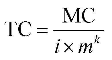 | (3) |
which allows for predicting the pXRF determined concentrations for infinitely thick samples using m and MC as inputs.
Besides the matrix effect caused by samples with intermediate-thickness which can be corrected as per eqn (3), the matrix effect caused by the use of soil mode for elemental analysis of organic samples may also cause less accurate results.2,34 Previous research suggests that a SLR model can effectively correct for the matrix effect and improve the accuracy of the results.2,29,34
Here, a SLR model was used to approximate the relationship between concentrations determined using pXRF and ICP-MS, respectively. The linear regression model was described using eqn (4):
| y = ax + b | (4) |
| [pXRF readings] = a[ICP − MS determined concentrations] + b | (5) |
with constants a and b determined using pXRF concentrations and ICP-MS results for the 39 samples in the calibration dataset. This equation then allows for adjustment of pXRF data for the 10 validation dataset samples whereby the final results are comparable with the ICP-MS results. eqn (5) was then converted to eqn (6):
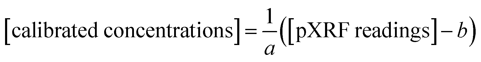 | (6) |
which is simplified to eqn (7) as:
| [calibrated concentrations] = p[pXRF readings] + d | (7) |
The CPDs for light elements are quite low (mm level) and a thickness of 1 cm seems to be thick enough.38,39,50 Thus, heavy elements were targeted in the present research. This is because the variation between pXRF determined concentrations for heavier elements (with higher CPDs) and mass thickness (sample mass per unit area) should be easier to observe.
Sample preparation
The 49 samples used for this pilot study consist of fungi, vegetation, and animal tissues (Table 1). All samples were oven-dried at 60 °C for 72 h to remove moisture. Next, the dried samples were ground to pass through a 250 μm sieve. The grinding time was adjusted according to the toughness of the samples. For example, the leech samples were ground for ∼6 min ensuring that over 95% leech sample particles passed through a 250 μm sieve. For mushroom samples, the grinding time was adjusted to ∼3 min.| Fungi (n = 17) | Vegetation (n = 16) | Animal tissues (n = 16) |
|---|---|---|
| a Purchased from a market in Weihe County, Harbin City, China. b Collected from the Bailing Cu–Zn deposit area in A'cheng District, Harbin City, China. c Purchased online at Taobao China. d Purchased from the Anguo Traditional Chinese Medicine (TCM) Market, Anguo City, China. | ||
| Pholiota nameko (n = 2)a | Leaf of Salix matsudana Koidz (n = 1)b | Leech (n = 3)d |
| Lepista nuda (n = 10)b | Leaf of Rhamnus davurica Pall (n = 1)b | Oyster (n = 2)c |
| Lentinula edodes (n = 2)a | Leaf of Sorbaria sorbifolia (n = 1)b | Shrimp (n = 2)c |
| Suillus luteus (n = 1)a | Straw of Oryza sativa L. (rice) (n = 3)b | Codfish (n = 1)c |
| Pleurotus citrinopileatus sing (n = 1)a | Leaf of Cirsium japonicum (n = 1)b | Salmon (n = 1)c |
| Panellus serotius (n = 1)a | Purple potato (n = 1)c | Pork liver (n = 2)c |
| Cocoa powder (n = 1)c | Goose liver (n = 1)c | |
| Matcha powder (n = 1)c | Chicken liver (n = 3)c | |
| Spices (ginger; citrus peel; white pepper) (n = 3)a | Lamb liver (n = 1)c | |
| Ginseng (n = 1)c | ||
| Carrot (n = 1)c | ||
| Spinach (n = 1)c | ||
Measurement methods
A Niton XL3t 950 (Thermo Fisher Scientific) pXRF spectrometer was used for elemental analysis following the methodology reported by Weindorf and Chakraborty.7 The instrument was equipped with a silicon drift detector (SDD) and an X-ray tube with a maximum voltage/current of 50 kV/40 μA and an Ag anode target excitation source. The diameter of the detection window was 8 mm. The dried and ground organic samples were placed in a sample cup with a diameter of 23 mm and a height of 25 mm. The sample cup was placed in a test stand with a thin polyethylene film protecting the aperture of the pXRF spectrometer from the powered organic samples. Soil mode was used in this study, as established in previous studies used to determine element concentrations in various organic samples.2,34 Fe, Cu, Zn, and As were determined under the main range scanning condition (50 keV and 40 μA) with a dwell time of 30 s; low and high energy ranges were disengaged. Each sample was scanned to produce 20 replicates. “System self-check” was performed to monitor spectral interference.51 “System self-check” is a factory calibration check used for confirming that the instrument is operating within resolution and stability tolerance (e.g., no shifts in energy line positions, regions of interest, or shift in gain control due to temperature changes).52 For quality assurance (monitoring signal drift), analysis of a certified reference material (CRM) (CRM Soil 180–649 supplied by Thermo Fisher Scientific) was conducted within every four samples runs. Elemental recovery percentages (PXRF determined/CRM reported) for As, Zn, Ni, Fe, Mn, Cr, K, and Ba were: 81–115%, 83–95%, 104–226%, 95–97%, 70–84%, 94–132%, 70–75%, and 72–88%, respectively. Notably, the certified As concentration in CRM 180–649 is 10.5 mg kg−1; pXRF readings near the limit of detection (LOD) are often less accurate.51The samples were subjected to ICP-MS analysis at ALS Minerals.53 To this end, the samples were digested using a HNO3/HCl acid mixture for 8 h at 20 °C. The digestion vessels were then transferred to a EG 20A-PLUS hotplate produced by LabTech (85 °C for 15 min and then 115 °C for 2 h). After digestion, when the vessel cooled to room temperature, HCl acid was added. Lastly, the prepared samples underwent ICP-MS analysis. A PerkinElmer Elan 6000 instrument was used for ICP-MS analysis. The LODs of the ICP-MS method for Fe, Cu, Zn, and As are 1 mg kg−1, 0.01 mg kg−1, 0.1 mg kg−1, and 0.005 mg kg−1, respectively. ICP-MS measurement accuracy was confirmed by measuring certified reference materials (GL-03 – leaves from Eucalyptus tree supplied by ALS Global Brisbane) at regular intervals. The certified values for Fe, Cu, Zn, and As in reference material GL-03 are 103 mg kg−1, 3.37 mg kg−1, 14.7 mg kg−1, and 0.293 mg kg−1, respectively. The recovery percentages (ICP-MS determined/CRM reported) for Fe, Cu, Zn, and As were 102.9–106.8%, 97.3–107.1%, 98.0–106.1%, and 100.3–106.5%, respectively. Furthermore, replicate ICP-MS measurements were conducted on random samples to observe the standard deviations of the ICP-MS measurements. Standard deviations (and relative standard deviations) of replicate measurements can reflect the uncertainty of ICP-MS analysis. The average relative standard deviations of replicate ICP-MS measurements were 4.00%, 2.02%, 1.61%, and 2.76% for Fe, Cu, Zn, and As, respectively.
Procedures and pXRF analysis
To determine the constants i and k in eqn (2), experiments were conducted as follows. The dried and ground organic samples were progressively added to sample cups and underwent pXRF analysis. As an example, for a mushroom sample (YHM-3-F), 0.256 g of the sample was added to a sample cup, and then the sample cup was lightly tapped on a table by hand for ∼40 seconds (∼30 times). This process ensures homogeneity of the sample in the sample cup. The table was covered with a piece of plain paper to prevent potential contamination to the film sealing the sample cup. Then the prepared sample was subjected to pXRF analysis. The sample mass in the sample cup was increased to 0.549 g, and subjected to pXRF analysis again. The sample mass in the sample cup was progressively increased to ∼3.1–3.5 g, since pXRF determined concentrations of the target elements varied little when the sample mass in the sample cup reached ∼3 g. The pXRF determined concentrations for the sample with higher mass (all >3.1 g) in the sample cup (with a diameter of 2.3 cm) were regarded as “infinitely thick” samples. The sample mass per unit area was calculated as per eqn (8): | (8) |
Calibration and performance verification
The samples were randomly split into an ∼80% calibration set (39 samples) and a ∼20% validation set (10 samples) a priori. The constants i and k in eqn (2) and (3) were calculated through experiments of samples in the calibration set, which allows for correction of the matrix effect caused in the analysis of intermediate-thickness samples.Constants p and d can be calculated from constants a and b (slopes and intercepts of the SLR equations between ICP-MS and pXRF determined concentrations for infinitely thick samples in eqn (4)) as per eqn (7), which corrects the error caused by analyzing organic materials using soil mode. Therefore, successful calibration of the pXRF determined concentrations of organic materials with intermediate thickness should combine eqn (3), (7) and (9) as follows:
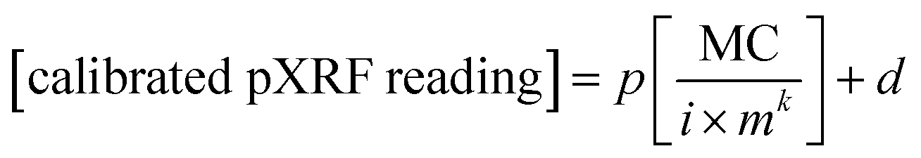 | (9) |
To evaluate the effects of calibrations, the relative errors (REs) [calibrated pXRF reading] were calculated. The RE was defined as per eqn (10) as:
 | (10) |
Results and discussion
Standardized pXRF determined concentrations versus sample mass per unit area (surface density)
Standardized pXRF determined Fe concentrations decreased with mass per unit area in a power law relationship (Fig. 1a). The standardized pXRF Fe concentrations in samples with low sample mass in the sample cup (mass per unit area) were significantly higher than those for “infinitely-thick” samples. For example, the measured Fe concentration for lamb liver was 1197.3 mg kg−1 with a sample mass of 0.119 g in the sample cup (0.0286 g cm−2), while the measured Fe concentration for the sample with infinite-thickness was 118.3 mg kg−1. The significant overestimation of Fe concentrations in samples with low sample mass indicates that the algorithm in pXRF analyzers incorrectly calculated the Fe concentrations and the original pXRF determined concentrations for intermediate-thick samples are not reliable. The values of constants i and k in eqn (5) were 0.770 and −0.651 for Fe, respectively (Fig. 1a). The coefficient of determination (R2) was 0.802, indicating a good correlation, especially considering that Fe concentrations for nearly 1/3 of samples were <200 mg kg−1 (∼twofold of the Fe LOD).51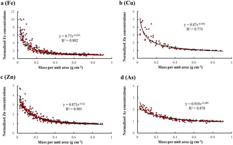 | ||
| Fig. 1 Relationships between the normalized portable X-ray fluorescence (pXRF) concentrations (measured pXRF concentrations for samples with different values of sample mass per unit area normalized by the concentrations of the infinitely thick samples) of Fe (a), Cu (b), Zn (c), and As (d) and the sample mass per unit area (surface density). | ||
Fig. 1b shows the relationship between the standardized pXRF determined concentrations for Cu and sample mass per unit area. The calibration set only contains 10 samples due to the inherent low Cu concentrations in the samples. The values of constants i and k were 0.87 and −0.491 for Cu, respectively (Fig. 1b). The R2 value for the Cu relationship was 0.774. Notably, Cu concentrations for four samples were <60 mg kg−1 and close to the LOD for Cu (∼20 mg kg−1). The R2 values increased to 0.900 after removing the four samples.
Fig. 1c shows the relationship between the standardized pXRF determined concentrations for Zn and sample mass per unit area. The values of constants i and k were 0.871 and −0.420 for Zn, respectively (Fig. 1c). Zinc concentrations were detected in all 39 samples in the calibration set and the LOD for Zn was <12 mg kg−1. The correlation was better for Zn with an R2 value of 0.901, suggesting that the proposed regression model (eqn (5)) fitted quite well; the calibration model (eqn (8)) should have strong potential to correct the effect caused by sample thickness. The strong correlation for Zn was likely due to the robust sensitivity for Zn detection via pXRF and the relatively high Zn concentration in the samples used for calibration.54
The standardized pXRF As concentrations also decreased with increasing sample mass per unit area with an R2 value of 0.878 (Fig. 1d). The values of constants i and k were 0.919 and −0.289 for As, respectively. The law's exponent (constant k) for As was the highest among those of all studied elements, which means the overestimation of As concentrations by pXRF in samples with low sample mass was less significant.
If the normalized concentration (MC/TC) is set at 1.01, then x represents the mass per unit area (surface density) which caused only a 1% overestimation of pXRF determined concentrations in the infinitely thick samples. This can be roughly regarded as the minimum mass per unit area of the infinitely thick samples under pXRF analysis (in which the X-rays are fully absorbed). According to the functions given in Fig. 1, the minimum mass per unit area causing full X-ray absorption was 0.659 g cm−2, 0.738 g cm−2, 0.703 g cm−2, and 0.721 g cm−2 for Fe, Cu, Zn, and As, respectively. Theoretically, the critical penetration depths of X-rays (also stands for sample mass per unit area if density is a constant) should increase with increasing atomic number.37,55 However, the calculated minimum sample mass per unit area which fully absorbs X-rays is greater for Cu than for Zn. This is due to the difference between the sample set for Cu and Zn: the set for Cu only contains 10 samples, while the set for Zn contains all 39 samples. If the same set was applied for Zn, the calculated minimum sample mass per unit area (surface density) would change to 0.730 g cm−2, very close to that of Cu (0.738 g cm−2), which might be explained by random errors or the limited sample size.
PXRF determined concentrations versus ICP-MS determined concentrations for “infinitely thick” samples
As shown in Fig. 2, the pXRF determined concentrations for Fe, Cu, Zn, and As were all strongly correlated with the ICP-MS determined concentrations. The R2 values were 0.922, 0.960, 0.940, and 0.925 for Fe, Cu, Zn, and As, respectively, which were slightly higher than the R2 values reported by McGladdery et al. (Fe: 0.74; Zn: 0.93; Cu: 0.82)34 and the R2 values reported by Turner et al. (Cu: 0.862; Zn: 0.959; As: 0.976).44 The particle size (<0.25 mm) in the present study was much smaller than those in the study carried out by McGladdery et al. (<2 mm), causing a higher degree of homogeneity and a higher R2 value.34,56 However, the R2 values for all studied elements were slightly lower than those reported by Zhou et al.,2 in which the elemental concentrations of dried and ground leech samples were determined using pXRF (Fe: 0.99; Cu: 1.00; Zn: 0.94; As: 0.95). This is likely because metal concentrations in leech samples can be high (e.g. CFe > 3500 mg kg−1); high-concentration samples may have elevated the R2 values.2 The slopes (95% confidence limits) for Fe, Cu, Zn, and As were 1.078 ± 0.121, 1.416 ± 0.235, 1.472 ± 0.123, and 1.267 ± 0.209, respectively. In this case, systemic errors were observed for Cu and Zn (and possibly As), whose slopes were different from 1. Overestimation of pXRF determined concentrations was likely due to the use of soil mode in the elemental determination of organic materials.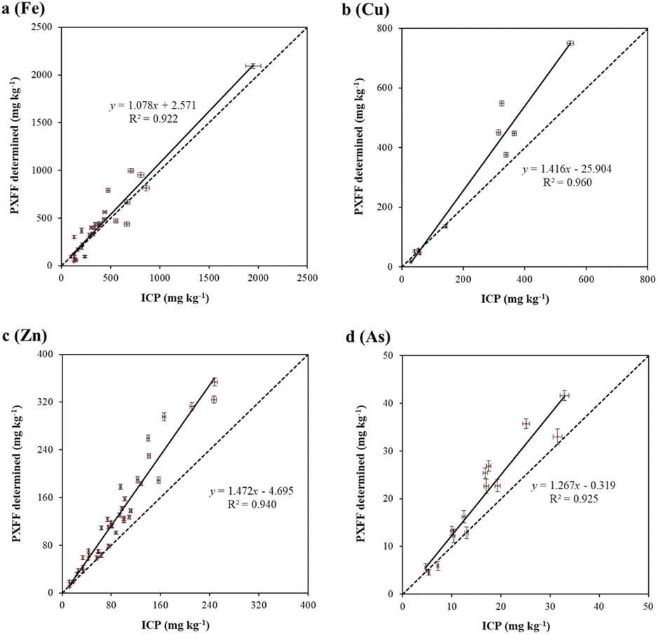 | ||
Fig. 2 Plots showing portable X-ray fluorescence (pXRF) vs. inductively coupled plasma mass spectroscopy (ICP-MS) determined Fe (a), Cu (b), Zn (c), and As (d) concentrations (mean ± SD) for 39 organic samples. The solid line represents the best-fitting line of ordinary least squares regression and the dotted line represents the 1![[thin space (1/6-em)]](https://www.rsc.org/images/entities/char_2009.gif) :1 line. :1 line. | ||
Overall, the correlation between ICP-MS determined concentrations and pXRF determined concentrations is quite solid, especially considering that the samples were of different species. This further demonstrates that different types of organic materials (fungi, vegetation, and animal tissues) may be regarded as a universal matrix in pXRF analysis; calibrations based on the same SLR models are then applicable for organic materials. Development of an organic mode suitable for analysis of organic materials is highly recommended to equipment manufacturers and further testing on a broader array of organic matrices is suggested to further refine the proposed universal organic matrix for pXRF analysis.
Validation of calibration models
Given the strong correlation between standardized pXRF determined concentrations and sample mass per unit area, as well as the correlation between pXRF and ICP-MS determined concentrations, eqn (9) was used to predict the elemental concentrations determined using ICP-MS in 10 samples of the validation set. The constants i and k can be obtained from the power-law functions given in Fig. 1. The constants p and d were calculated from constants a and b as per eqn (7). Constants a and b are slopes and intercepts of the linear regression equations in Fig. 2. Then, the calibration models for predicting elemental concentrations determined by ICP-MS in organic materials with intermediate thickness were obtained using eqn (11)–(14) as follows: | (11) |
 | (12) |
 | (13) |
 | (14) |
The concentrations found using eqn (11)–(14) were then compared with those determined using ICP-MS; relative errors were calculated. The relationship between the sample mass per unit area and relative errors is shown in Fig. 3.
 | ||
| Fig. 3 Relationships between the relative errors of calibrated Fe (a), Cu (b), Zn (c), and As (d) concentrations and sample mass per unit area. | ||
Better performance was observed for Zn (Fig. 3c). PXRF was effective in the analysis of all 10 samples of the validation set. The REs of the predicted Zn concentrations were all <18% in 105 measurements, with an average of 8.9% (Fig. 3c). PXRF only detected As in three samples. The REs of the predicted As concentrations were <22% in 35 measurements (<20% for 95% measurements), with an average RE of 9.1% (Fig. 3d). However, the validation results for Fe and Cu were even worse. For Fe, pXRF was effective for seven samples. The REs of the predicted Fe concentrations were <34% in 61 measurements, with an average RE of 11.5%. The less robust validation results for Fe were expected, since pXRF is more sensitive for heavier elements due to their higher excitation energy.7 The fluorescence yield characterizing the elements is poor for light elements due to the limited number of electrons contained therein. As such, only high concentrations of light elements (e.g. Na, Mg, and Al) are detectable via pXRF. Furthermore, as shown in Fig. 1a, Fe concentrations may vary dramatically with sample mass per unit area in thin samples; a tiny change of sample mass may cause huge variations in the Fe concentration determined by pXRF, which coincided with the results obtained by Fleming et al.57 Another source of errors may arise during experiments, since the powdered sample may not be uniformly distributed in the sample cup; geometrical placement is important in XRF analysis.47 For Cu, pXRF was only effective for three samples. The REs of the predicted Cu concentrations were generally <30% in 33 measurements, with an average RE of 11.5%. Such results may be explained by the limited number of samples of the calibration set.
Conclusions
This research introduced a calibration model allowing pXRF to quantify Fe, Cu, Zn, and As concentrations in organic materials (fungi, vegetation, and animal tissues) with intermediate thickness. The calibration model was divided into two parts:The pXRF determined concentrations of Fe, Cu, Zn, and As in intermediate-thickness samples were found to decrease with increasing sample mass per unit area (surface density) in the sample cup in a power-law relationship. The coefficients of determination (R2) of the power-law regression models were 0.802, 0.774, 0.901, and 0.878 for Fe, Cu, Zn, and Zn, respectively. The derived mass-correction model allows correction for the matrix effect caused by analyzing intermediate-thickness samples.
The pXRF determined concentrations for infinitely-thick samples were linearly correlated with the ICP-MS determined concentrations. The R2 values of the SLR model were 0.922, 0.960, 0.940, and 0.925 for Fe, Cu, Zn, and Zn, respectively. The SLR calibration model allows pXRF determined concentrations for infinitely-thick samples to predict ICP-MS based concentrations.
The mass-correction model and the SLR calibration model were employed to calibrate the matrix effect caused by analyzing the intermediate-thickness organic samples (10 samples of the validation set). The corrected pXRF determined concentrations were compared with the ICP-MS determined concentrations. The validation results were very good for Zn and As, and acceptable for Fe and Cu. The REs of the predicted Zn, As, Fe, and Cu concentrations were <18%, <22%, <34%, and <30%, respectively. The validation results suggest that pXRF was capable of quantifying trace metal concentrations in organic materials with intermediate thickness. In future analysis, the sample mass per unit area (surface density) should be considered as the factor controlling pXRF determined concentrations rather than the sample thickness, since sample density may not be uniform in different organic matrices.
Conflicts of interest
There are no conflicts to declare.Acknowledgements
This research was jointly supported by the National Key Research and Development Program of China (No. 2018YFE0204200), the National Natural Science Foundation of China (42050103), the China Geological Survey Project (20190459), Fundamental Research Funds for the Central Universities, the China Scholarship Council – Macquarie University Scholarship, and the IAMG Founders Scholarship.References
- M. Rouillon and M. P. Taylor, Can field portable X-ray fluorescence (pXRF) produce high quality data for application in environmental contamination research?, Environ. Pollut., 2016, 214, 255–264 CrossRef CAS PubMed.
- S. Zhou, Q. Cheng and D. C. Weindorf, et al., Elemental assessment of dried and ground samples of leeches via portable X-ray fluorescence, J. Anal. At. Spectrom., 2020, 35(11), 2573–2581 RSC.
- J. B. Jones Jr and V. W. Case, Sampling, handling, and analyzing plant tissue samples, Soil Test. Plant Anal., 1990, 3, 389–427 Search PubMed.
- J. Søndergaard and C. J. Jørgensen, Field Portable X-Ray Fluorescence (pXRF) Spectrometry for Chemical Dust Source Characterization: Investigations of Natural and Mining-Related Dust Sources in Greenland (Kangerlussuaq Area), Water, Air, & Soil Pollution, 2021, 232(4), 1–17 Search PubMed.
- A. E. Steiner, R. M. Conrey and J. A. Wolff, PXRF calibrations for volcanic rocks and the application of in-field analysis to the geosciences, Chem. Geol., 2017, 453, 35–54 CrossRef CAS.
- S. Chakraborty, B. Li and D. C. Weindorf, et al., Use of portable X-ray fluorescence spectrometry for classifying soils from different land use land cover systems in India, Geoderma, 2019, 338, 5–13 CrossRef CAS.
- D. C. Weindorf and S. Chakraborty, Portable X-ray fluorescence spectrometry analysis of soils, Soil Sci. Soc. Am. J., 2020, 84(5), 1384–1392 CrossRef CAS.
- S. Chakraborty, T. Man and L. Paulette, et al., Rapid assessment of smelter/mining soil contamination via portable X-ray fluorescence spectrometry and indicator kriging, Geoderma, 2017, 306, 108–119 CrossRef CAS.
- B. T. Ribeiro, D. C. Weindorf and B. M. Silva, et al., The Influence of Soil Moisture on Oxide Determination in Tropical Soils via Portable X-ray Fluorescence, Soil Sci. Soc. Am. J., 2018, 82(3), 632–644 CrossRef CAS.
- J. Yang, Z. Yuan and E. Grunsky, et al., Analysis of geochemical patterns in a soil profile over mineralized bedrock, Geochem.: Explor., Environ., Anal., 2022, 22(3), geochem2021-088 CrossRef.
- Z. Yuan, H. Chang and S. Zhou, et al., In situ monitoring of elemental losses and gains during weathering using the spatial element patterns obtained by portable XRF, J. Geochem. Explor., 2021, 229, 106842 CrossRef CAS.
- Z. Yuan, Q. Cheng and Q. Xia, et al., Spatial patterns of geochemical elements measured on rock surfaces by portable X-ray fluorescence: application to hand specimens and rock outcrops, Geochem.: Explor., Environ., Anal., 2014, 14(3), 265–276 CrossRef CAS.
- J. Kagiliery, S. Chakraborty and B. Li, et al., Portable X-ray fluorescence analysis of water: thin film and water thickness considerations. EQA-International, J. Environ. Qual., 2021, 45, 27–41 Search PubMed.
- D. Pearson, S. Chakraborty and B. Duda, et al., Water analysis via portable X-ray fluorescence spectrometry, J. Hydrol., 2017, 544, 172–179 CrossRef CAS.
- C. R. Ward, S. J. Kelloway and J. Vohra, et al., In situ inorganic analysis of coal seams using a hand-held field-portable XRF Analyser, Int. J. Coal Geol., 2018, 191, 172–188 CrossRef CAS.
- J. Kagiliery, S. Chakraborty and A. Acree, et al., Rapid quantification of lignite sulfur content: Combining optical and X-ray approaches, Int. J. Coal Geol., 2019, 216, 103336 CrossRef CAS.
- G. Sánchez-Pomales, T. K. Mudalige and J. H. Lim, et al., Rapid determination of silver in nanobased liquid dietary supplements using a portable X-ray fluorescence analyzer, J. Agric. Food Chem., 2013, 61(30), 7250–7257 CrossRef PubMed.
- C. A. Hoffmann, J. O. Sarturi and D. C. Weindorf, et al., The use of portable X-ray fluorescence spectrometry to measure apparent total tract digestibility in beef cattle and sheep, J. Anim. Sci., 2020, 98(3), skaa048 CrossRef PubMed.
- M. Nicholas and P. Manti, Testing the applicability of handheld portable XRF to the characterisation of archaeological copper alloys, 2014 Search PubMed.
- S. Piorek, Alloy identification and analysis with a field-portable XRF analyser, Portable X-Ray Fluoresc. Spectrom., 2008, 98–140 CAS.
- D. E. B. Fleming, S. R. Bennett and C. J. Frederickson, Feasibility of measuring zinc in human nails using portable X-ray fluorescence, J. Trace Elem. Med. Biol., 2018, 50, 609–614 CrossRef CAS PubMed.
- D. E. B. Fleming, S. L. Crook and C. T. Evans, et al., Assessing arsenic in human toenail clippings using portable X-ray fluorescence, Appl. Radiat. Isot., 2021, 167, 109491 CrossRef CAS PubMed.
- J. Johnson, Accurate measurements of low Z elements in sediments and archaeological ceramics using portable X-ray fluorescence (PXRF), J. Archaeol. Method Theory, 2014, 21(3), 563–588 CrossRef.
- R. H. Tykot, N. M. White, J. P. Du Vernay, et al., Advantages and disadvantages of pXRF for archaeological ceramic analysis: Prehistoric pottery distribution and trade in NW Florida, Archaeological Chemistry VIII, American Chemical Society, 2013, pp. 233–244 Search PubMed.
- A. McWhirt, D. C. Weindorf and Y. Zhu, Rapid analysis of elemental concentrations in compost via portable X-ray fluorescence spectrometry, Compost Sci. Util., 2012, 20(3), 185–193 CrossRef CAS.
- D. C. Weindorf, R. Sarkar and M. Dia, et al., Correlation of X-ray fluorescence spectrometry and inductively coupled plasma atomic emission spectroscopy for elemental determination in composted products, Compost Sci. Util., 2008, 16(2), 79–82 CrossRef.
- D. R. Cohen, E. J. Cohen and I. T. Graham, et al., Geochemical exploration for vertebrate fossils using field portable XRF, J. Geochem. Explor., 2017, 181, 1–9 CrossRef CAS.
- A. Turner and K. R. Solman, Analysis of the elemental composition of marine litter by field-portable-XRF, Talanta, 2016, 159, 262–271 CrossRef CAS PubMed.
- S. Zhou, D. C. Weindorf and Q. Cheng, et al., Elemental assessment of vegetation via portable X-ray fluorescence: sample preparation and methodological considerations, Spectrochim. Acta, Part B, 2020, 174, 105999 CrossRef CAS.
- T. I. McLaren, C. N. Guppy and M. K. Tighe, A rapid and nondestructive plant nutrient analysis using portable X-ray fluorescence, Soil Sci. Soc. Am. J., 2012, 76(4), 1446–1453 CrossRef CAS.
- S. H. G. Silva, B. T. Ribeiro and M. B. B. Guerra, et al., pXRF in tropical soils: Methodology, applications, achievements and challenges, Adv. Agron., 2021, 167, 1–62 Search PubMed.
- S. Zhou, Z. Yuan and Q. Cheng, et al., Rapid in situ determination of heavy metal concentrations in polluted water via portable XRF: using Cu and Pb as example, Environ. Pollut., 2018, 243, 1325–1333 CrossRef CAS PubMed.
- S. Zhou, Z. Yuan and Q. Cheng, et al., Quantitative analysis of iron and silicon concentrations in iron ore concentrate using portable X-ray fluorescence (XRF), Appl. Spectrosc., 2020, 74(1), 55–62 CrossRef CAS PubMed.
- C. McGladdery, D. C. Weindorf and S. Chakraborty, et al., Elemental assessment of vegetation via portable X-ray fluorescence (PXRF) spectrometry, J. Environ. Manage., 2018, 210, 210–225 CrossRef CAS PubMed.
- E. Marguí, I. Queralt and M. Hidalgo, Application of X-ray fluorescence spectrometry to determination and quantitation of metals in vegetal material, TrAC, Trends Anal. Chem., 2009, 28(3), 362–372 CrossRef.
- E. Margui, R. Padilla and M. Hidalgo, et al., High-energy polarized-beam EDXRF for trace metal analysis of vegetation samples in environmental studies, X-Ray Spectrom., 2006, 35(3), 169–177 CrossRef CAS.
- P. J. Potts, O. Williams-Thorpe and P. C. Webb, The bulk analysis of silicate rocks by portable X-ray fluorescence: effect of sample mineralogy in relation to the size of the excited volume, Geostand. Newsl., 1997, 21(1), 29–41 CrossRef CAS.
- B. T. Ribeiro, D. C. Weindorf and C. S. Borges, et al., Foliar analysis via portable X-ray fluorescence spectrometry: experimental considerations, Spectrochim. Acta, Part B, 2021, 186, 106320 CrossRef CAS.
- S. Reidinger, M. H. Ramsey and S. E. Hartley, Rapid and accurate analyses of silicon and phosphorus in plants using a portable X-ray fluorescence spectrometer, New Phytol., 2012, 195(3), 699–706 CrossRef CAS PubMed.
- R. Sitko, Quantitative X-ray fluorescence analysis of samples of less than ‘infinite thickness’: difficulties and possibilities, Spectrochim. Acta, Part B, 2009, 64(11–12), 1161–1172 CrossRef.
- R. Sitko, Empirical coefficients models for X-ray fluorescence analysis of intermediate-thickness samples, X-Ray Spectrom., 2005, 34(1), 11–18 CrossRef CAS.
- R. Sitko, Theoretical influence coefficients for correction of matrix effects in X-ray fluorescence analysis of intermediate-thickness samples, X-Ray Spectrom., 2006, 35(2), 93–100 CrossRef CAS.
- R. Sitko and J. Jurczyk, Determination of absorption correction by the ‘two masses’ method for XRF analysis of intermediate samples, X-Ray Spectrom., 2003, 32(2), 113–118 CrossRef CAS.
- A. Turner, H. Poon and A. Taylor, et al., In situ determination of trace elements in Fucus spp. by field-portable-XRF, Sci. Total Environ., 2017, 593, 227–235 CrossRef PubMed.
- A. Bull, M. T. Brown and A. Turner, Novel use of field-portable-XRF for the direct analysis of trace elements in marine macroalgae, Environ. Pollut., 2017, 220, 228–233 CrossRef CAS PubMed.
- D. E. B. Fleming, M. R. Gherase and M. Anthonisen, Calibrations for measurement of manganese and zinc in nail clippings using portable XRF, X-Ray Spectrometry, 2013, 42(4), 299–302 CrossRef CAS.
- M. R. Gherase and D. E. B. Fleming, A calibration method for proposed XRF measurements of arsenic and selenium in nail clippings, Phys. Med. Biol., 2011, 56(20), N215 CrossRef CAS PubMed.
- M. Rincheval, D. R. Cohen and F. A. Hemmings, Biogeochemical mapping of metal contamination from mine tailings using field-portable XRF, Sci. Total Environ., 2019, 662, 404–413 CrossRef CAS PubMed.
- U. Sharma, K. Van Delinder and J. L. Gräfe, et al., Investigating methods of normalization for X-ray fluorescence measurements of zinc in nail clippings using the TOPAS Monte Carlo code, Appl. Radiat. Isot., 2022, 182, 110151 CrossRef CAS PubMed.
- E. K. Towett, K. D. Shepherd and B. Lee Drake, Plant elemental composition and portable X-ray fluorescence (pXRF) spectroscopy: quantification under different analytical parameters, X-Ray Spectrometry, 2016, 45(2), 117–124 CrossRef CAS.
- Z. Yuan, Q. Cheng and H. Chang, et al., In situ geochemistry of dyke-marble interfaces obtained by portable X-ray fluorescence (pXRF) spectroscopy: Implications for sources of ore-forming materials in the Baiyinnuo'er Zn–Pb deposit, inner Mongolia, China, Appl. Geochem., 2020, 122, 104770 CrossRef CAS.
- G. Hall, A. Buchar and G. Bonham-Carter, Quality control assessment of portable XRF analysers: development of standard operating procedures, performance on variable media and recommended uses, CAMIRO Project 10E01 report, 2011 Search PubMed.
- ALS Geochemistry Technical Note, Biogoechemistry ALS METHODS, 2020 Search PubMed.
- C. S. Borges, D. C. Weindorf and G. S. Carvalho, et al., Foliar elemental analysis of Brazilian crops via portable X-ray fluorescence spectrometry, Sensors, 2020, 20(9), 2509 CrossRef CAS PubMed.
- J. Yang, Z. Zhang and Q. Cheng, Resolution enhancement in micro-XRF using image restoration techniques, J. Anal. At. Spectrom., 2022, 37(4), 750–758 RSC.
- Y. Sapkota, L. M. McDonald and T. C. Griggs, et al., Portable X-ray fluorescence spectroscopy for rapid and cost-effective determination of elemental composition of ground forage, Front. Plant Sci., 2019, 10, 317 CrossRef PubMed.
- D. E. B. Fleming, M. N. Nader and K. A. Foran, et al., Assessing arsenic and selenium in a single nail clipping using portable X-ray fluorescence, Appl. Radiat. Isot., 2017, 120, 1–6 CrossRef CAS PubMed.
| This journal is © The Royal Society of Chemistry 2022 |