Quantification of C, H, N and O in polymers using WDXRF scattering spectra and PLS regression depending on the spectral resolution

Abstract

A new approach to determine the elements carbon, hydrogen, nitrogen and oxygen (CHNO) in polymers by wavelength-dispersive X-ray fluorescence analysis (WDXRF) in combination with partial least squares (PLS) regression was explored. The quantification of CHNO was achieved by using the Rayleigh and Compton scattering spectra of an Rh X-ray tube from 84 different polymers. Concealed differences of the corresponding scattering spectra could be utilized to quantify CHNO in a multivariate manner. It was shown that the developed model was capable of determining these commonly non-measurable matrix elements in polymers using WDXRF. Furthermore, the influence of spectral resolution, which is given by the collimator and the crystal, on the prediction of CHNO was explored in this study. It was found that minimal spectral resolution led to the most accurate CHNO predictions. Information about matrix composition could be used to improve so-called semi-quantitative XRF methods based on fundamental parameters (FP) for the analysis of plastics, soil or other samples with high organic content.

---

Introduction

X-ray fluorescence analysis (XRF) is one of the most versatile analytical techniques for studying the elemental composition of solid and liquid matrices. In many instances, time-consuming and costly sample preparation steps are not necessary. Using XRF, more than 80 elements can be identified almost simultaneously. There is an ongoing development of new hardware, e.g. high-resolution energy detectors in the field of energy-dispersive XRF (EDXRF)^1–3 and new X-ray optics and instrumentations.⁴ Moreover, advancements in software development provide chemometric opportunities for XRF, which previously were not possible.^5–8 These are significant factors for the ongoing success of this technology. In addition to the well-established applications such as the metal or cement industry, XRF is increasingly applied in the ever-growing field of plastics.^9–11 Due to stricter laws and regulations, e.g. Restriction of Hazardous Substances (2002/95/EG), Waste Electrical and Electronic Equipment (2002/96/EG) and Directive on the Safety of Toys (2009/48/EC), the elemental analysis of synthetic products in all areas of the value chain (polymer compounding, polymer production, manufacturer and consumers) is becoming more significant.¹²

Two approaches are employed for quantification in XRF: the empirical methods and the so-called semi-quantitative methods. The empirical method relates XRF signals to a known sample composition with certified reference materials (CRM). The so-called semi-quantitative methods are based on a theoretical approach to quantify elements using fundamental parameters (FP).¹³ In real-life applications, an enormous variety of polymer types with varying filler and additive combinations are employed to tailor the properties according to the application's demand. Unfortunately, so far, only a limited number of polymeric CRM are available, which are based on polyethylene (PE),¹⁴ unsaturated polyester resin (UP),^15,16 polycarbonate (PC),¹⁷ polyvinyl chloride (PVC),¹⁸ polypropylene (PP)¹⁸ and acrylonitrile butadiene styrene (ABS).^19,20 Furthermore, these CRM cover only limited element compositions and are restricted to small ranges of element concentrations. To perform quantification based on empirical methods, countless calibration standards based on suitable polymers and element compositions would be required.

A more applicable procedure to quantify elements in polymers is based on algorithms operating with FP (absorption coefficient, emission coefficient, etc.) of the elements.^21,22 This approach models the interactions between elements and allows for the calculation of all element concentrations in a given sample. A prerequisite for obtaining reliable results by this theoretical quantification procedure is that all elements present in a sample have to be detectable by the XRF measurement.¹³

Most polymers contain the so-called low Z elements carbon, hydrogen, nitrogen or oxygen (CHNO) in total amounts greater than 95 wt%. These elements are often undetectable or insufficiently detectable by XRF. Subsequently, the quantification of elements in a polymeric matrix by employing FP methods often leads to inaccurate quantification. The common approach to overcome this problem is to add an assumed polymeric matrix for the FP method. When no further information concerning the material is available, CH₂ (PE) is assumed as a sum parameter for plastic materials in software programs. When no information on CHNO matrix composition is available, the FP method cannot be applied to all polymers due to varying concentrations of CHNO within the polymers and additives (fillers, catalyst residuals, light stabilizers, heat stabilizers, UV stabilizers, plasticizers, antioxidants, etc.). Inaccurate matrix information may lead to great deviations for elements of higher atomic numbers, e.g. Ca, Ti, Fe or Zn, due to matrix effects. Several procedures were developed to determine the elemental composition of the polymers by considering low Z elements via the coherent scattering signal, incoherent scattering signals and ratios thereof. However, these approaches were not eligible to quantify the correct composition of the polymer matrix.^23–27 Therefore, it is mandatory to identify the exact low Z element composition (CHNO) of the organic matrix to reliably quantify the additional elements present in plastic materials via FP methods.

Aidene et al. used energy dispersive X-ray fluorescence (EDXRF) with X-ray tube excitation in combination with partial least squares (PLS) modeling to determine the hydrogen, carbon and oxygen (CHO) concentrations of various thermoplastic samples.²⁸ In another study, the authors employed a monochromatic excitation to calculate the carbon and hydrogen concentrations.²⁹ It was found that the precision was similar to polychromatic excitation.

The purpose of this study was to maximize the precision of CHNO quantification and assess the dependence on spectral resolution (i.e. crystal-collimator) used in WDXRF. The Rayleigh and Compton scattering spectra of different polymers were studied employing PLS regression to quantify CHNO concentrations utilizing WDXRF.

Coherent and incoherent scattering

The coherent or elastic scattering of X-rays, known as Rayleigh scattering, describes the interaction of an incoming X-ray photon with a firmly bound electron. In this process, the incident photon is scattered without changing its wavelength or frequency. Therefore, no energy loss occurs. The intensity of the Rayleigh scattering is a function of the atomic number and the wavelength.^30,31

The incoherent or inelastic scattering of X-rays, known as Compton scattering, is also induced by an interaction of an incoming X-ray photon with an electron. In contrast to the Rayleigh scattering, the impact of the incoming photon leads to the removal of a loosely bound electron out of its orbital by transferring a part of its energy to this electron. This energy transfer induces a scattering of the collided photon and results in an increased wavelength.^32–35

Compton scattering is inversely proportional to the mean atomic number of a given sample. Therefore, a sample composed of low Z elements yields a high intensity of Compton scattering. Thus, the shape or pattern of scattering spectra must contain information regarding the composition of elements with low atomic numbers.

Theoretical approach

The attenuation of X-ray photons passing through matter can mainly be described by two physical processes: absorption and scattering. Absorption can be described by the photoelectric absorption coefficient τ. The scattering part is given by the scattering coefficient σ, which is composed of the coherent scattering coefficient σ_coh and incoherent scattering coefficient σ_incoh. The combination of these quantities yields the mass absorption coefficient μ_m, which describes the attenuation of X-ray photons. The mass absorption coefficient μ_m of an entire sample is given by the mass fractions w_i of all present elements in the sample and the corresponding absorption and scattering coefficients (eqn (1)).

The interaction of X-ray photons with low Z elements, e.g. CHNO, mostly causes scattering of X-ray photons. The effect is increased at higher energies of involved X-ray photons, e.g. K-series of X-ray tube anodes like Rh (Fig. 1), Pd or W. This consideration implies that the composition of the elements CHNO is related to the specific X-ray scattering pattern of the respective polymer. Therefore, it may be possible to determine the composition of an organic polymer quantitatively. In this study, the material-specific scattering spectra are analyzed to quantify CHNO by exploiting concentration and X-ray energy-dependent attenuation of X-rays.

Fig. 1 Rh-Kα X-ray tube scattering spectra (coherent and incoherent) of several materials of same sample masses.

Materials and methods

Preparation of calibration materials

A set of 29 thermoplastics and 55 thermoset polymers were prepared and employed for this study. It was essential for the investigations that all polymers were undoped; thus, the average mass absorption coefficients in the energy region of interest are in a comparable range. Otherwise, doped elements of higher atomic numbers influence scattering spectra and quantification of CHNO by the proposed procedure will lead to reduced accuracies.³⁶ Undoped polymers merely consisted of the polymer itself and were preferably not filled or stabilized in any way. The majority of the thermoset plastics consisted of custom-made, unsaturated polyester resins (UP made of fumaric acid combined with different polyolic compounds), epoxy resins (EP) and polyurethanes (PUR) (Table 1). The polymers were intentionally selected to cover a wide range of materials with varying CHNO compositions.

Table 1 Polymer types used for sample preparation

Thermoplastics
10 samples of PA (polyamide)	2 samples of PP (polypropylene)
1 sample of POM (polyoxymethylene)	1 sample of PR (phenolic resin)
2 samples of PC (polycarbonate)	5 samples of HD/LD-PE (high/low-density polyethylene)
3 samples of ABS (acrylonitrile butadiene styrene)	1 sample of HI-PS (high impact polystyrene)
1 sample of PMMA (poly-(methyl methacrylate))	1 sample of TPU (thermoplastic polyurethane)
1 sample of PET (polyethylene terephthalate)	1 sample of PBT (polybutylene terephthalate)

---

Thermoset plastics
6 samples of EP (epoxy resin)
43 samples of UP (unsaturated polyester resin)
6 samples of PUR (polyurethane)

---

All thermoplastic samples, including the thermoplastic polyurethane sample, were prepared by molding the polymers using an automatic mounting press equipped with a 40 mm mold cylinder (SimpliMet 3000, Buehler, Düsseldorf, Germany). The thermoset plastics (UP, EP) were made by mixing the acid and the polyolic component systems beforehand. Then, each mixture was cast in a customized aluminum mold equipped with two cavities. The samples were hardened in these cavities at standard room temperature (20 °C). Photographs of the mold can be found in ESI (Fig. S1).† Then, a grinder–polisher (Alpha, Buehler, Düsseldorf, Germany) was applied to adjust the resulting sample thickness and mass. The produced plastic samples had masses of 5.0 ± 0.1 g.

XRF scattering spectra

A wavelength dispersive X-ray spectrometer (S4 Pioneer, Bruker AXS, Karlsruhe, Germany) equipped with an Rh X-ray tube was used to obtain the scattering spectra of the 84 prepared polymer samples. The scan measurement settings are listed in Table 2. The X-ray tube was operated at electrical power of 3 kW (60 kV, 50 mA). In this study, the dependence of CHNO predictions on the spectral resolution was investigated. A hypothesis was that a higher spectral resolution might result in improved CHNO concentration predictions. This improvement could be attributed to a better separation of coherent scattering signals and incoherent scattering signals. A low spectral resolution was realized by LiF (200) crystal combined with a 0.46° collimator. This setup yielded maximum X-ray intensity in this study. A medium spectral resolution was realized by LiF (220) crystal combined with a 0.23° collimator. A high spectral resolution was realized by LiF (420) crystal combined with a 0.12° collimator. This setup yielded minimal X-ray intensity in this study. A NaI (Tl) scintillation counter was used as a detector for acquisition for all spectral resolutions investigated. For each spectral resolution, 300 s acquisition time was defined in the measuring method. The angular step size was 20% of the collimator aperture. Furthermore, the recorded range was broader than the pure scattering region. Therefore, for each spectral resolution, an effective acquisition time was used (Table 2). The measurements were performed using different LiF crystals (2d values: LiF (200) 0.4026 nm, LiF (220) 0.2848 nm and LiF (420) 0.1801 nm). The conversion of 2θ to photon energy was conducted using the Bragg condition. Records on 2θ were converted to photon energy to better compare with spectra of energy-dispersive devices. In the following analysis, the Rh tube scattering region from 17–24 keV was used.

Table 2 XRF measurement parameters and settings

XRF spectrometer		S4 Pioneer (Bruker AXS)
X-ray tube target (anode)		Rhodium (Rh)
Voltage/current		60 kV/50 mA
Energy range		17–24 keV
Crystal/collimator	Low resolution	LiF (200)/0.46°
	Medium resolution	LiF (220)/0.23°
	High resolution	LiF (420)/0.12°
Acquisition time	Low resolution	80.6 s
	Medium resolution	176 s
	High resolution	241 s
Measuring spot (mask)		34 mm
Measuring mode		Vacuum

---

Elemental analysis

CHNO reference concentrations of the investigated plastic samples are needed for calibration of the WDXRF device. The CHNO concentrations of the 84 prepared samples were determined by organic elemental analysis by combustion. The device vario Macro (Elementar, Langenselbold, Germany) was used at Bundesanstalt für Materialforschung und -prüfung, Berlin, Germany. Duplicate analysis was conducted for sample masses of 50–70 mg. The samples were packed in Sn foil and then fed to the catalytic combustion column at 960 °C in an oxygen stream. The reburning column was operated at 900 °C and the reduction column was operated at 830 °C. The samples' oxygen concentrations could not be measured and were balanced to 100 wt%.

PLS regression model

At first, the data set was split randomly into a training set (67%, 56 samples) and a testing set (33%, 28 samples). The training set data is used for validating the PLS model, i.e. to identify the optimal number of PLS components (refer to the next paragraph) to employ. The testing data is hold-out in the validation process and only used for assessment of the models' generalization capability.³⁷

For the investigation of the scattering spectra, a PLS algorithm was applied (Statistics Toolbox of MATLAB®, R2009a, The MathWorks Inc.). The base for multivariate regression modeling is the multiple linear regression approach (eqn (2)).

Y = X·B + E (2)

The matrix Y is composed of CHNO concentrations data, and the matrix X corresponds to the intensities of the recorded WDXRF scattering tube spectra. The regression coefficients are given by matrix B. These regression coefficients can be used to interpret the created regression model, because they are associated with corresponding photon energy, respectively. The regression residuals are given by the matrix E. In PLS regression, the matrices X and Y are decomposed into smaller submatrices for scores and loadings. For this step, the data are transformed on calculated PLS components. These PLS components can be seen as a new coordinate system. Concerning the scores, the new axes capture maximum variance in the spectral data X and the CHNO concentrations Y. Furthermore, the new axes maximize the covariance and, thus, the correlation between X and Y. The determination of the optimal PLS component number is crucial in preventing the overfitting of the training data. Thus, deviations between predictions of validation data and corresponding reference data can be minimized.³⁷ Detailed descriptions of the PLS method can be found in the literature.^38–41

Pre-processing of data records may have a significant influence on the regression's performance.⁷ The PLS algorithm, used in MATLAB®, applied mean-centering of each feature, i.e. energy, prior to PLS decomposition. Further pre-processing, e.g. z-scaling,³⁸ was not necessary for this study. When z-scaling was applied, the R² metrics for testing data were less than or equal compared to unscaled data.

A single PLS model was created to quantify CHNO concentrations instead of utilizing individual PLS models for C, H, N and O concentrations. This single PLS model procedure is advantageous due to improved model interpretability, e.g. concerning regression coefficients, and especially when target element concentrations are correlated.⁴⁰

The calibration model quality on training data and predictions of hold-out testing samples is given by the root mean square error (RMSE, eqn (3)). The optimal number of PLS components was determined with the aid of RMSE and leave-one-out (LOO) cross-validation (CV). A schematic representation of the CV procedure can be found in ESI (Fig. S2).† The testing set was not used for CV and was completely hold-out during training of the model. Therefore, it was possible to see how well the cross-validated PLS model could generalize the data by prediction of the testing set.

In RMSE, elemental analysis concentrations are represented by y_i and predicted concentrations via the PLS regression model are represented by ŷ_i. The number of considered samples equals N. The arithmetic average RMSE (avg. RMSE) gives a single metric to assess the model performance for a given spectral resolution of CHNO concentration predictions (eqn (4)). Additionally, a weighted average RMSE (wavg. RMSE) is calculated (eqn (5)).

In the wavg. RMSE, the individual RMSE_i for CHNO quantifications are weighted concerning the corresponding average mass fraction ȳ_i in the training set or the testing set, respectively. Therefore, in wavg. RMSE the individual RMSE, especially for N concentrations, are down-weighted due to comparatively low N concentrations in all 84 plastic samples. The wavg. RMSE is a more important metric compared to avg. RMSE when assessing the CHNO concentration prediction quality. For a correct ascertainment of μ_m (eqn (1)), high accuracy in the determination of the CHNO elements is more important for elements with high concentrations in the polymer than for elements with very low concentrations.

Results and discussion

The scattering spectra (Fig. 2) and the corresponding elemental analysis of the 84 polymer samples (Fig. 3) were chosen as the basis for the PLS model. Elemental analysis data can be found in ESI (Table S1).† The CHNO concentrations were predicted from WDXRF scattering spectra (Table S2).†

Fig. 2 XRF scattering spectra of 84 polymer samples, (a) low spectral resolution, (b) medium spectral resolution and (c) high spectral resolution, random colors to show minor intensity differences between spectra (see Table 2 for spectral resolutions).

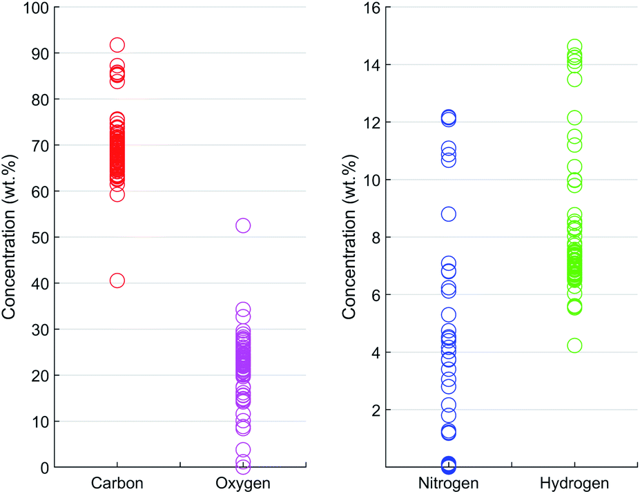Fig. 3 Concentrations of CHNO in the 84 prepared calibration samples (CHN by elemental analysis, O balanced to 100 wt%).

To obtain an optimal PLS model, CV was applied for the training set data. After CV, the final model was fitted with the optimal number of PLS components. The model predicted the CHNO concentration for training and testing data. The predictions were compared with reference values in terms of avg. RMSE and wavg. RMSE.

Cross-validation

The CV procedure was used to determine the optimal number of PLS components. In total, 56 folds were generated randomly. Corresponding average RMSE was calculated for training data and validation data (Fig. S2).† For the high spectral resolution, a distinct local minimum in RMSE (CV) was determined at 4 PLS components (Fig. 4). The RMSE (CV) curve leveled off at 5 PLS components for low and medium spectral resolutions. An increase in the PLS component number resulted in increased model complexity without improving the recovery of validation data (overfit). In contrast, a reduction of the PLS component number resulted in an RMSE too large for validation data (underfit). Thus, the optimal number of PLS components was 5 for low and medium spectra resolution and 4 for high spectral resolution. The RMSE for training data monotonically decreased with the number of PLS components. This decrease was due to the models' adaption to the training data and decreased generalization capabilities for new samples when the number of PLS components was too high.³⁷

Fig. 4 RMSE for CHNO prediction for cross-validation (CV) and training set in dependence of PLS component number for different spectral resolutions. This figure is used to estimate the optimal PLS component number that is given by minimum RMSE in CV.

The CV results (Fig. 4) show that for increasing spectral resolution, the RMSE for training data decreased for all numbers of PLS components, respectively. This supports the hypothesis that a better spectral separation of coherent and incoherent scattering signals may lead to improved performance in the prediction of CHNO concentrations. For the validation data, this tendency was not observed, but the inverted tendency. For reducing spectral resolution, the RMSE (CV) was decreasing. This implies that the generalization capability of the corresponding PLS model was improved for lower spectral resolutions. It should be noted that this was the result of CV. In CV, samples are used for training the PLS model as well as for validating the PLS model to optimize for the number of PLS components. Thus, information from validation samples was also used for training in other CV folds (Fig. S2).† An improved approach, which avoids this information reuse, was based on evaluating predicted CHNO concentrations from the hold-out testing data by the final PLS models (Table 3). The evaluation of CHNO predictions from testing data enabled an improved analysis because the model did not adapt to testing data.

Table 3 Assessment of the CHNO quantification procedures using cross-validated PLS regression models for training and testing data using RMSE metrics

Spectral resolution	Element	Training set (wt%)			Testing set (wt%)
		RMSE	avg. RMSE	wavg. RMSE	RMSE	avg. RMSE	wavg. RMSE
Low	C	1.8	1.5	1.6	1.8	1.5	1.6
	H	0.22			0.3
	N	2.4			2.4
	O	1.7			1.3
Medium	C	1.2	1.0	1.1	2.0	1.7	1.9
	H	0.17			0.4
	N	1.4			2.5
	O	1.2			2.0
High	C	1.3	1.7	1.4	2.0	1.8	1.9
	H	0.25			0.54
	N	3.2			2.6
	O	2.2			2.0

---

Cross-validated PLS model

Once the optimal numbers of PLS components for each spectral resolution were found by CV, the PLS models were built by fitting the model to the entire training data set. The trained PLS models were used to predict the CHNO concentration of the training set and for the testing set (Table S2†). In a recovery plot, the predicted CHNO concentrations are plotted against the measured CHNO concentrations for all spectral resolutions (Fig. 6). Plots of CHNO predictions in a low concentration range (below 10 wt%) are given in ESI (Fig. S3).† It was observed that for all spectral resolutions, the predicted C, H and O concentrations were in good agreement with the measured concentrations from elemental analysis. In the case of N, the results were less accurate. One of the reasons could be the low sample fraction of about 35% containing N (29 out of 84 samples). Furthermore, the N concentrations in these polymers vary in a rather narrow range (0–12.1 wt%). In contrast, H covered a comparable concentration range (4–15 wt%), but was present in all of the 84 investigated samples.

The regression coefficients of the trained model enabled the interpretation of energy regions that are significant for extracting the respective CHNO concentration (Fig. 5, spectra in grey). Energies associated with high absolute values of regression coefficients substantially influence the particular target element concentration. The algebraic sign of regression coefficients indicates the direction of influence, i.e. positive coefficients are positively related with target concentrations and vice versa. It was shown that the quantification of C concentration was mainly influenced by the inflection points of the incoherent Rh-Kα signal, i.e. higher number of recorded counts affected an increase in C concentration. In contrast, the energy region around the incoherent scattering peak maximum 18.75–19.5 keV showed the inverted effect; thus, a higher number of recorded counts affected a decrease in C concentration. The magnitude of the decreasing effect was smaller due to lower absolute regression coefficients. In contrast to the quantification of C concentration, other energy regions influenced the quantification of N. The PLS predictions of N concentrations were positively correlated with the incoherent Rh-Kα scattering peak and coherent Rh-Kα scattering peak. This was given by high regression coefficients in these energy regions. On the other hand, the incoherent Rh-Kβ peak and coherent Rh-Kβ peak were negatively correlated with the PLS predictions of N concentrations.

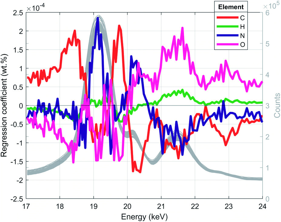Fig. 5 PLS regression coefficients and XRF spectra for low spectral resolution (grey lines, right axis). This figure reveals energy regions that are used to extract corresponding CHNO concentration.

Fig. 6 Recovery plot for CHNO quantification by PLS models, results for training and testing data are shown, diagonals plotted to guide the reader's eye (see Table 2 for spectral resolutions).

The dependence of CHNO quantifications on spectral resolution was investigated. The avg. RMSE and wavg. RMSE of predicted CHNO concentrations and elemental analysis were calculated for training and testing data to assess the PLS models' prediction capabilities (Table 3). It was found that avg. RMSE and wavg. RMSE for training data was less than for testing data concerning high spectral resolution and medium spectral resolution. For low spectral resolution avg. RMSE and wavg. RMSE were about the same. It can be concluded that for high and medium spectral resolution the RMSE for training data is overly optimistic because the RMSE for training data was lower compared to those of testing data. For low spectral resolution, there was no difference in the evaluation of training or testing data.

The higher spectral resolution, i.e. improved separation of coherent scattering signals and incoherent scattering signals, did not improve CHNO predictions. Besides the spectral resolution, other essential factors describe the quality of spectra for CHNO predictions, e.g. the total counts recorded. The counting statistics are more precise when more counts are recorded.³⁰ The emission and detection of X-ray photons can be described by a Poisson distribution.^30,42 Therefore, the standard deviation of detected photons due to statistical fluctuation in spectra can be estimated by the square root of the number of detected photons, respectively. To compare the 3 spectral resolutions in terms of counting statistics, total signal intensity was calculated by summation over the energies and all samples for each spectral resolution. At low spectral resolution, the total signal intensity of scattering spectra for all investigated samples was 2.08 × 10⁹ counts. For medium spectral resolution, the total signal intensity was 1.64 × 10⁹ counts and for high spectral resolution signal intensity was 0.48 × 10⁹ counts. To compare the counting statistics for spectral resolutions, the square roots and ratios thereof were formed. The ratio of roots was 2.1 to 1.8 to 1 in the order of low, medium and high spectral resolution. Additionally, the ratio of wavg. RMSE for CHNO concentration predictions and elemental analysis of the testing set was 0.83 to 0.97 to 1, also in the order of low, medium and high spectral resolution. As a result, the lowest spectral resolution was best suited for predictions of testing data due to the increased precision in counting statistics and reduced wavg. RMSE for testing set data. Thus, the lowest spectral resolution could generalize the data best and had the best performance in the prediction of CHNO concentrations from WDXRF scattering spectra.

Various combinations of CHNO concentrations may result in similar mass absorption coefficients μ_m. However, the presented PLS regression model can resolve the varying concentrations. The arithmetic mean μ_m in the Rh-Kα scattering region (17–24 keV) for all samples were calculated based on only the CHNO compositions to illustrate this. The total cross sections (Compton and Rayleigh cross-sections from Elam et al.⁴³ and photoionization cross sections from Kissel⁴⁴) were calculated using xraylib⁴⁵ 4.0.0. The mean μ_m, reference CHNO concentrations and predicted CHNO concentrations for the low spectral resolution were plotted. An interactive plot is given in the ESI.†

Conclusions

In this study, a new approach for the quantification of typically non-measurable matrix elements in polymers (CHNO) by the use of the WDXRF was developed. Calibrations for CHNO concentrations of polymers were generated by PLS regression, employing scattering spectra of the X-ray tube. By this procedure, WDXRF was able to determine the CHNO concentrations of polymers, and no further measurements of CHNO concentrations, e.g. by elemental analysis, are necessary. The quantified CHO concentrations using the PLS model were in good agreement with the measured concentrations from elemental analysis. Remarkably, H could be reliably determined by WDXRF, although H does not show any X-ray fluorescence. The quantification of H could be realized indirectly via scattering. In contrast to the good agreement of CHO with elemental analysis data, the predicted N concentrations were less accurate. This is explained by the low number of samples containing N.

In this study, only undoped polymers were investigated. Elements with atomic numbers greater than 8 have a considerable influence on the scattering spectra. In plastics, these elements are commonly applied, e.g. as components in additives to manufacture certain material properties. To incorporate this influence on the scattering spectra, a further study was carried out.³⁶ In this further study, additional polymers containing varying amounts of elements in a broad range of atomic numbers are considered for PLS regression modeling. The CHNO quantification is also possible in doped plastics when the doped plastics are also considered in the training data. Besides the CHNO quantification based on WDXRF spectra, the proposed procedure is also applicable for EDXRF spectra (including a micro XRF device and a handheld XRF device).³⁶

In FP-based quantification procedures, the quantification of CHNO could be employed to analyze low Z material, e.g. plastics or biomass. The matrix composition could directly be used for semi-quantitative determination of higher Z elements, e.g. Ti, Fe, Zn, Br, Pb or Cd, from the same scan measurement.

Author contributions

Conceptualization: G. W., S. H., M. K., M. O.; data curation: M. B., G. W.; formal analysis: M. B., G. W.; funding acquisition: G. W., S. H., M. K.; investigation: G. W.; methodology: M. B., G. W., S. H., M. K.; project administration: G. W.; resources: S. H., M. K., M. O.; software: M. B., G. W.; supervision: M. K., M. O.; validation: M. B., G. W.; visualization: M. B., G. W.; writing – original draft: M. B., G. W.; writing – review & editing: M. B., G. W., S. H., M. K., M. O.

Conflicts of interest

There are no conflicts to declare.

Acknowledgements

The authors thank Bundesministerium für Bildung und Forschung, Germany for funding (grant number 1756X08). The authors thank Sierra Pitman for proofreading this manuscript.

References

1. S. Piorek, Proc. Int. Conf. Asian Green Electron., 2005, 7–13.
2. D. L. Anderson, J. AOAC Int., 2010, 93, 683–693.
3. N. Miskolczi, C. Varga and L. Bartha, Muanyag Gumi, 2009, 46, 235–239.
4. M. Haschke, Laboratory Micro-X-Ray Fluorescence Spectroscopy, Springer International Publishing, 2014.
5. V. Panchuk, I. Yaroshenko, A. Legin, V. Semenov and D. Kirsanov, Anal. Chim. Acta, 2018, 1040, 19–32.
6. V. Panchuk, V. Semenov, A. Legin and D. Kirsanov, Anal. Chem., 2018, 90, 5959–5964.
7. F. R. dos Santos, J. F. de Oliveira, E. Bona, G. M. C. Barbosa and F. L. Melquiades, Spectrochim. Acta, Part B, 2021, 175, 106016.
8. J.-M. Roger and J.-C. Boulet, J. Chemom., 2018, 32, e3045.
9. F. Puype, J. Samsonek, V. Vilímková, Š. Kopečková, A. Ratiborská, J. Knoop, M. Egelkraut-Holtus, M. Ortlieb and U. Oppermann, Food Addit. Contam., Part A, 2017, 34, 1767–1783.
10. A. Turner, Mar. Pollut. Bull., 2017, 124, 286–291.
11. A. Turner, Chemosphere, 2021, 263, 128087.
12. K. R. Beebe, R. J. Pell and M. B. Seasholtz, Chemometrics: A Practical Guide, Wiley, New York, 1998.
13. R. M. Rousseau, Open Spectrosc. J., 2009, 3, 31–42.
14. A. Lamberty, W. Van Borm and P. Quevauviller, Fresenius' J. Anal. Chem., 2001, 370, 811–818.
15. K. Nakano, T. Nakamura, I. Nakai, A. Kawase, M. Imai, M. Hasegawa, Y. Ishibashi, I. Inamoto, K. Sudou, M. Kozaki, A. Tsuruta, A. Ono, K. Kakita and M. Sakata, Anal. Sci., 2006, 22, 1265–1268.
16. K. Nakano, K. Tsuji, M. Kozaki, K. Kakita, A. Ono and T. Nakamura, Adv. X-Ray Anal., 2006, 49, 280–286.
17. K. J. Lee, Y. J. Lee, Y. R. Choi, J. S. Kim, Y. S. Kim and S. B. Heo, Anal. Chim. Acta, 2013, 758, 19–27.
18. M. Ohata and A. Hioki, Anal. Sci., 2013, 29, 239–246.
19. M. Ostermann, A. Berger, C. Mans, C. Simons, S. Hanning, A. Janssen and M. Kreyenschmidt, Accredit. Qual. Assur., 2011, 16, 515–522.
20. C. Simons, C. Mans, S. Hanning, A. Janssen, M. Radtke, U. Reinholz, M. Ostermann, M. Michaelis, J. Wienold, D. Alber and M. Kreyenschmidt, J. Anal. At. Spectrom., 2010, 25, 40–43.
21. J. Sherman, Spectrochim. Acta, 1955, 7, 283–306.
22. J. Sherman, Adv. X-Ray Anal., 1958, 1, 231–252.
23. H. K. Bothe, Fresenius' J. Anal. Chem., 1986, 324, 27–32.
24. C. W. Dwiggins Jr, Anal. Chem., 1961, 33, 67–70.
25. C. M. Johnson and P. R. Stout, Anal. Chem., 1958, 30, 1921–1923.
26. G. V. Pavlinsky, A. Y. Dukhanin, E. O. Baranov and A. Y. Portnoy, J. Anal. Chem., 2006, 61, 654–661.
27. R. Sitko, J. Anal. At. Spectrom., 2006, 21, 1062–1067.
28. S. Aidene, V. Semenov, D. Kirsanov, D. Kirsanov and V. Panchuk, Spectrochim. Acta, Part B, 2020, 165, 105771.
29. S. Aidene, V. Semenov, D. Kirsanov, D. Kirsanov and V. Panchuk, Measurement, 2021, 172, 108888.
30. R. E. v. Grieken and A. A. Markowicz, Handbook of X-Ray Spectrometry, Marcel Dekker, Inc., New York, 2002.
31. G. R. Lachance and F. Claisse, Quantitative X-ray Fluorescence Analysis: Theory and Application, Wiley, Chichester, New York, 1995.
32. A. H. Compton and A. W. Simon, Phys. Rev., 1925, 26, 290–299.
33. A. H. Compton, Phys. Rev., 1923, 22, 409–413.
34. A. H. Compton, Philos. Mag., 1923, 46, 897–911.
35. A. H. Compton, Proc. Natl. Acad. Sci. U. S. A., 1925, 11, 303–306.
36. G. Wacker, PhD thesis, TU Bergakademie Freiberg, 2015.
37. T. Hastie, R. Tibshirani and J. Friedman, The Elements of Statistical Learning: Data Mining, Inference, and Prediction, SpringerNew York, 2nd edn, 2017.
38. M. Otto, Chemometrics, Wiley-VCH, 3rd edn, 2017.
39. P. Filzmoser, S. Serneels, R. Maronna and P. J. Van Espen, Comprehensive Chemometrics, Elsevier, pp. 681–722,  DOI:10.1016/B978-044452701-1.00113-7.
40. S. Wold, M. Sjostrom and L. Eriksson, Chemom. Intell. Lab. Syst., 2001, 58, 109–130.
41. R. G. Brereton, Chemometrics: Data Driven Extraction For Science, John Wiley & Sons, 2nd edn, 2018.
42. B. Beckhoff, B. Kanngießer, N. Langhoff, R. Wedell and H. Wolff, Handbook of Practical X-Ray Fluorescence Analysis, Springer Berlin Heidelberg, 2007.
43. W. T. Elam, B. D. Ravel and J. R. Sieber, Radiat. Phys. Chem., 2002, 63, 121–128.
44. L. Kissel, Radiat. Phys. Chem., 2000, 59, 185–200.
45. T. Schoonjans, A. Brunetti, B. Golosio, M. Sanchez del Rio, V. A. Solé, C. Ferrero and L. Vincze, Spectrochim. Acta, Part B, 2011, 66, 776–784.

---

Footnote

† Electronic supplementary information (ESI) available. See DOI: 10.1039/d1ja00412c

---