Techno-economic and greenhouse gas emission assessment of carbon negative pyrolysis technology

Abstract

Carbon-negative energy removes carbon dioxide from the atmosphere while providing energy to society. The pyrolysis-biochar platform achieves carbon-negative energy by producing bio-oil as an energy product and biochar as a carbon sequestration agent. This study evaluates the economic and environmental performance of conventional fast pyrolysis (FP) and autothermal pyrolysis (ATP) systems with and without pretreatment of three kinds of biomass to produce sugars, phenolic oil, and biochar as valuable products while achieving carbon negative emissions. Techno-economic (TEA) and life cycle analysis (LCA) results show minimum sugar selling prices (MSSP) as low as zero while achieving significant carbon dioxide removal from the atmosphere. Comparison of these systems to direct air capture (DAC) shows that the pyrolytic systems are competitive both in terms of net carbon dioxide (CO₂) removal per unit of energy consumption and cost of removing CO₂ which ranges between $30 to −$139 per ton CO₂ removed.

---

1 Introduction

The 2018 report of the International Panel on Climate Change (IPCC) recommends that by 2030 carbon dioxide emissions be reduced to 49% of 2017 emissions and attain carbon neutrality by 2050 to limit global temperature rise to 1.5 °C.¹ The 2021 IPCC report suggests expedited reductions in GHG emissions with a goal of reaching net-zero CO₂ emissions.² Strategies for reducing greenhouse gas emissions, thus far, are not sufficient to reach this goal, leading to calls for removal of carbon dioxide from the atmosphere.³

Several carbon removal strategies have been proposed. In terms of economic incentives for implementing them, some are limited to income from sequestering carbon. Examples include afforestation and direct air capture (DAC). Afforestation is the reestablishment of forests for the purpose of carbon removal. Some companies already use afforestation to off-set their carbon emissions.⁴ It is relatively inexpensive, but there are limits to the amount of land that can be dedicated to this practice. Direct air capture uses large fans to flow air across sorbents that remove carbon dioxide and recover it as pure gas streams destined for geological storage.⁵ One of the main roadblocks for DAC is the cost of CO₂ removal. The process is very energy-intensive, requiring around 4.5–17 kW h of energy for capturing 1 kg of CO₂ from the atmosphere.^6,7

Other approaches to carbon removal also generate electric power or fuels, providing additional economic incentives for adoption.⁸ Prominent examples of so-called carbon negative energy include bioenergy with carbon capture and sequestration (BECCS) and the pyrolysis-biochar platform. Originally developed to capture CO₂ emissions from coal gasification power plants, BECCS substitutes biomass for coal to achieve carbon negative energy. Because growing biomass fixes carbon from the atmosphere, that part of the biogenic carbon converted to carbon dioxide during gasification and sequestered represents net removal of carbon dioxide from the atmosphere.⁹ The syngas from biomass gasification can be used for either electric power generation or production of fuels. The pyrolysis-biochar platform produces bio-oil as an energy product and sequesters biogenic carbon in the form of a carbonaceous solid known as biochar.^10,11 Rather than sequestering it in geological deposits, this recalcitrant solid is applied to soils where it provides ecosystem services. Each of these approaches has advantages and challenges.⁸ Most prominently, gasification can sequester a larger portion of biogenic carbon than pyrolysis but is challenged by the economics and reliability of CO₂ storage.⁸ Pyrolysis is attractive for its ability to be deployed at small scales well matched to the distributed nature of biomass supply and has more attractive economics. This study explores the economics and environmental performance of a carbon negative energy system based on pyrolysis of biomass.

Fast pyrolysis is the thermochemical conversion of biomass with the potential production of a wide range of products, including biofuels, fermentable sugars, and biobased chemicals.^12–15 Although biofuels from fast pyrolysis appear to be economically attractive,^16–18 technical challenges have hindered its commercial adoption.^19,20 Among these challenges is difficulty in providing energy to the reactor as the process is scaled up.^21,22 Autothermal pyrolysis (ATP) was recently developed to overcome this challenge by admitting air into the pyrolysis reactor at equivalence ratios of around 0.06. Partial oxidation of some of the products of pyrolysis releases enough energy to sustain endothermic pyrolysis reactions.²¹ Autothermal pyrolysis simplifies reactor design and enables process intensification resulting in several-fold increase in reactor throughput. A novel application of ATP is the production of pyrolytic sugar, phenolic oil, and biochar to achieve carbon-negative energy.²³

The feasibility of producing cellulosic sugars from pyrolysis of lignocellulosic biomass has been demonstrated by removing or passivating naturally occurring alkali and alkaline earth metals (AAEM) in biomass, increasing the value of pyrolytic products.²⁴ Passivation is attractive as it avoids the difficulty of effectively removing AAEM from the biomass. The earliest passivation studies employed sulfuric acid as pretreatment to convert AAEM into thermally stable sulfate salts, preventing the metals from catalyzing pyranose and furanose ring fragmentation.²⁵ However, acid pretreatments can promote char agglomeration during pyrolysis, interfering with reactor operation.^26,27 A recent study by Rollag et al.²⁸ found that pretreatment with ferrous sulphate not only passivated AAEM but prevented char agglomeration, which was attributed to the ferrous ions serving as lignin depolymerization catalyst.

Pyrolytic sugars include pyranose and furanose monosaccharides but mostly the anhydrosugar levoglucosan from cellulose depolymerization.²⁷ Levoglucosan has a wide range of commercial applications such as fermentation to ethanol,²⁹ polymerization to bioplastics,³⁰ and upgrading to pharmaceuticals³¹ and green solvents.³² Techno-economic analysis (TEA) of an ATP-based biorefinery producing levoglucosan crystals estimated a minimum selling price of $1333 per MT, which is much less than its current market price of $50 per kg.³³ A TEA on solvent liquefaction as a pathway for production of fermentable sugars for fermentation to ethanol found the minimum fuel selling price (MFSP) ranged between $2.98 to $4.06 per gallon. A life cycle analysis (LCA) in the same study estimated GHG emissions from the resulting fuel were 25%–45% lower than for petroleum-derived gasoline.³⁴ In addition, an LCA of biobased levoglucosan estimated its global warming potential to be half that of petroleum-derived chemicals.³⁵ TEA and LCA of an integrated pyrolysis and anaerobic digestion system for production of ethanol and phenolic compounds estimated the MFSP to be $1.21 per gallon with net GHG emissions of −16.6 g CO_2e per MJ.¹³

Another major pyrolysis product is phenolic oil, consisting of a wide range of phenolic compounds derived from the thermal depolymerization of lignin in biomass.³⁶ Phenolic oil can be upgraded to fuels and other products.^16,37 Of particular interest in the present study is the use of phenolic oil in the production of an asphalt binder substitute known as bioasphalt.^38–40 Traditional asphalt, derived from petroleum, is a key building material around the world for roads and highways.⁴¹ Finding a biobased substitute for asphalt will be important as the use of fossil fuels is curtailed to mitigate climate change. Peralta et al.⁴⁰ described the use of biorenewable resources as bio-binders in the production of alternatives to asphalt. Raouf et al.³⁹ found that the rheological properties of bio-oil from switchgrass and bitumen binders made them feasible replacements for petroleum-based asphalt binders.

The environmental advantages of biobased binders have been previously investigated. Samieadel et al.⁴² reported GHG emissions of around 0.37 kg CO₂ eq. per kg for bioasphalt produced from hydrothermal liquefaction of pig manure slurry with the bioasphalt containing 10% bio-oil and 90% petroleum-based asphalt. Zhou et al.⁴³ reported LCA of a biochar modified bioasphalt with GHG emissions ranging between 0.16–0.19 kg CO₂ eq. per kg of product. Biobased binders appear to be economically attractive. Dang et al.³⁷ found that producing dextrose, calcium acetate, and bioasphalt from an integrated 2000 metric ton per day (MTPD) fast pyrolysis biorefinery processing woody feedstock has prospects for achieving an internal rate of return as high as 68%.

This study evaluates the techno-economic analysis (TEA) and life cycle analysis (LCA) of conventional fast pyrolysis (FP) and autothermal pyrolysis (ATP) biorefineries processing three different types of lignocellulosic biomass, namely corn stover (CS), red oak (RO) and yellow pine (YP). Both untreated biomass and biomass pretreated to enhance pyrolytic sugar production were evaluated. These carbon negative energy systems are compared to the economic and environmental performance of a direct air capture (DAC) plant.

2 Materials and methods

To support the TEA and LCA, process models of ATP and FP biorefineries were developed. Corn stover (CS), red oak (RO) and yellow pine (YP) were evaluated as potential feedstocks for these biorefineries. Four major product streams were modeled: levoglucosan-rich sugar; phenolic oil; biochar; and tail gas consisting of light oxygenated compounds and non-condensable gases, which are burned for process heat for the ATP scenario, while the light oxygenates are blended with phenolic compounds in case of the FP scenario. Outputs from this analysis included MSSP and extent and cost of carbon removal. Sensitivity and uncertainty analyses are employed to identify key cost and emission drivers and the probability of processes’ profitability. These pyrolysis-based carbon negative energy technologies are compared to direct air capture (DAC) of CO₂. This study is comprised of eight scenarios utilizing three kinds of lignocellulosic biomass in FP and ATP systems which are as follows:

i. Corn stover fed fast pyrolysis (CS FP) with no pretreatment

ii. Corn stover fed autothermal pyrolysis with no pretreatment (CS ATP, no PT)

iii. Corn stover fed autothermal pyrolysis with FeSO₄ pretreatment (CS ATP, PT)

iv. Red oak fed fast pyrolysis system (RO FP) with no pretreatment

v. Red oak fed autothermal pyrolysis with no pretreatment (RO ATP, no PT)

vi. Red oak fed autothermal pyrolysis with FeSO₄ pretreatment (RO ATP, PT)

vii. Yellow pine fed autothermal pyrolysis without any pretreatment (YP ATP, no PT)

viii. Yellow pine fed autothermal pyrolysis with FeSO₄ pretreatment (YP ATP, PT)

2.1 Autothermal pyrolysis (ATP) and conventional fast pyrolysis (FP) systems

This study was developed from experimental data generated at Iowa State University on conventional fast pyrolysis of untreated lignocellulosic biomass^28,44 and autothermal pyrolysis of biomass that was either untreatedor pretreated with ferrous sulfate for the purpose of enhancing sugar production.²⁸Table 1 shows the yields of sugar, phenolic oil, and biochar (kg kg⁻¹ input) from laboratory experiments for the different scenarios (other products not included in the table are non-condensable gases, light oxygenated compounds, and water). Conventional FP of yellow pine is not included in the analysis because no experimental data was available for this scenario.

Table 1 Yields of sugar, phenolic oil, and biochar and input of FeSO₄ for fast pyrolysis (FP) and autothermal pyrolysis (ATP) with and without biomass pretreatment and three kinds of biomass feedstock

Lignocellulosic biomass	Operating conditions	Sugar yield (wt% dry biomass)	Phenolic oil yield^a (wt% dry biomass)	Biochar yield (wt% dry biomass)	FeSO4 input (wt% dry biomass)	Source
a Includes phenolics recovered during cleaning of sugars.
Corn stover (CS)	FP	0.9	13.5	20.5	0.0	Elliot et al.^44 and Rollag et al.^28
	ATP, no PT	0.9	15.0	23.0	0.0
	ATP, PT	11.8	18.1	14.0	7.5
Red oak (RO)	FP	7.7	20.0	13.2	0.0	Dalluge et al.,^27 Elliot et al.^44 and Rollag et al.^28
	ATP, no PT	4.4	19.0	15.0	0.0
	ATP, PT	15.5	21.0	11.0	1.0
Yellow pine (YP)	ATP, no PT	5.4	18.0	14.0	0.0	Rollag et al.^28
	ATP, PT	19.0	19.4	17.0	1.0

---

Fig. 1 and 2 are flow diagrams of the FP and ATP processes to produce sugar, phenolic oil, and biochar. The two processes differ primarily in whether biomass is pretreated and how thermal energy is supplied to the process.

Fig. 1 Simplified flow diagram for conventional fast pyrolysis for the production of sugar, phenolic oil, and biochar production (adapted from Rover et al.³³).

Fig. 2 Simplified flow diagram of autothermal pyrolysis system for production of sugar, phenolic oil, and biochar production (adapted from Rover et al.³³).

2.1.1 Conventional fast pyrolysis (FP) scenario. As shown in Fig. 1, biomass is coarsely chopped, dried to 10% moisture content and further ground to 2–3 mm particle size. The biomass is fed to fluidized bed pyrolyzer to produce a product stream comprising of pyrolysis vapors, biochar and non-condensable gases (NCG). Gas cyclones separate biochar followed by condensers and electrostatic precipitators to recover heavy ends and light ends of bio-oil. The heavy ends consist of sugars and anhydrosugars (mostly levoglucosan) and phenolic compounds. The remaining non-condensable gases are reutilized along with natural gas (NG) to meet process heating requirements while the light oxygenates are further blended with phenolic oil. The heavy ends undergo a hot water wash to separate the water-soluble sugars and water-insoluble phenolic oligomers. The resulting sugar solution is contaminated with partially water-soluble phenolic monomers, which are removed in a resin adsorbent column. The separated phenolic monomers are combined with the phenolic oligomers recovered from the liquid–liquid extraction unit to produce a mixture called phenolic oil (PO). This product is sold as feedstock for production of bioasphalt.

2.1.2 Autothermal pyrolysis (ATP) scenario. As shown in Fig. 2, biomass is coarsely chopped and either dried to 10% moisture content and ground to 2–3 mm particle size (for the ATP, no PT cases in Table 1) or pretreated with ferrous sulfate solution before drying and further grinding (for the ATP, PT cases in Table 1). Pretreatment (FeSO₄) enhances sugar production, as described by Rollag et al.²⁸ The biomass is pyrolyzed in a fluidized bed in the presence of a small amount of air to achieve autothermal operation.²³ As with the FP scenario, a gas cyclone removes biochar from the product stream followed by a condenser and electrostatic precipitator to recover heavy ends of bio-oil. The light ends of bio-oil are not condensed but rather burned with the non-condensable gases in a furnace to provide process heat for drying biomass. As with the FP scenarios, the heavy ends are hot water washed to separate the sugar and phenolic oil. The raw sugar solution is passed through a resin column to remove phenolic monomers, which are combined with the phenolic oligomers. This product is sold as feedstock for production of bio-asphalt.

2.2 Process modelling

The pyrolysis systems were modeled with Aspen Plus™ assuming 250 MTPD of biomass processing capacity.⁴⁵ FP scenarios employ no further pretreatment of biomass (corn stover and red oak), while ATP scenarios have three instances (corn stover, red oak, and yellow pine) employing pretreatment and three without any pretreatment. All the ATP scenarios employ air at an equivalence ratio of 0.045 to support partial oxidation of pyrolysis products for the purpose of autothermally heating the pyrolysis reactor.

The major unit operations modeled include: (i) the pretreatment section where chopping, drying, and grinding of biomass occurs; (ii) the FP and ATP reactors; (iii) the cyclone separator to remove solid biochar from the pyrolysis vapors; (iv) the heavy ends recovery section where heavy ends are separated and condensed from NCG, light oxygenates, and water; (v) the sugar block that yields purified sugar solution from the heavy ends through liquid–liquid extraction and SMB unit; (vi) a steam generator block for the FP scenarios that burns non-condensable gases from the pyrolyzer along with natural gas to provide process heat to the system; and (vii) a furnace block for the ATP scenarios that burns NCG and light oxygenates to produce process heat for the drying section. Further details of the process model are available in Rover et al.³³

2.3 Techno-economic analysis (TEA)

TEA is a method for estimating a technology's economic feasibility and profitability using five fundamental components: process model design, equipment selection and sizing, economic analysis, process optimization, user interface.⁴⁶ In this study, TEA assumes a biorefinery facility employing FP and ATP of 250 MTPD of lignocellulosic biomass to produce primarily levoglucosan-rich sugar along with biochar and phenolic oil as byproducts. Most of the financial assumptions for the plant are based on data from Rover et al.³³ Installation factors for the project come from Peters et al.⁴⁷ Discounted cash flow rate of return (DCFROR) analysis was employed to evaluate the plant's economic viability. The plant life was assumed to be 10 years. The internal rate of return (IRR) was set at 10%. All the financial assumptions employed a 2015$ basis. Table 2 shows the key financial assumptions for quantifying the minimum fuel selling price (MSSP). The annual operating costs include labor, overhead, maintenance, and insurance.

Table 2 Key financial assumptions for a 250 ton per day biomass fast pyrolysis (FP) and autothermal (ATP) biorefinery producing sugar, phenolic oil, and biochar

Parameters	Assumptions
Equity	40%
Construction period	1 year
Plant life	10 years
Working capital	15% of fixed capital investment
Depreciation period	7 years, 200 double declining balance
Plant salvage value	0
Start-up time	0.5 years
Revenue and cost during startup	Revenue: 50% of mean annual revenues
	Revenues variable cost: 75% of mean annual variable costs
	Fixed costs: 100% of mean annual fixed costs
IRR	10%
Interest rate of financing	8% annually

---

The material, energy, and byproduct revenue costs are tabulated in Tables 3 and 4. According to the US Billion Ton report of 2016, the price of lignocellulosic woody biomass ranges between 36–73 per MT.⁴⁸ This study assumed an average price of $41 per MT for lignocellulosic biomass, as employed in previous studies.⁴⁹ Electricity for grinding biomass was assumed to be around 20 kW h per ton.⁵⁰ While the ATP system did not require external energy sources, the FP system required natural gas (NG) in the amount of 350 kW h per ton biomass processed⁵¹ at a cost of $0.005 per MJ ($5.68 per MMBTU) based on previous studies and market prices.⁵² The FeSO₄ used to pretreat biomass in some of the ATP scenarios is not recycled in the plant but incorporated into the biochar. The market price of FeSO₄ ranges between $520–650 per MT (per communication with Crown Technology, Inc. Aug. 29, 2019); we assumed $550 per MT. Biochar and phenolic oil revenue were assumed to be $80 per MT⁵³ and $500 per MT,^54,55 respectively. We assumed that 99% of the methanol used to regenerate the resin columns in sugar cleaning was recovered³⁴ with a replacement cost of $500 per MT.⁵⁶ The mass and energy balances for unit operations were obtained from the process model. The process model also provided operating conditions and performance parameters utilized for equipment selection and sizing purposes.

Table 3 Material and energy flows of a 250 ton per day fast pyrolysis (FP) and autothermal pyrolysis (ATP) biorefinery processing corn stover (CS), red oak (RO), or yellow pine (YP)

Materials & energy	Flowrate (MT per day)		Cost ($ per MT or kW h or MJ)
	FP	ATP
a Electricity price in $ per kW per h. b Natural gas price in $ per MJ.
Biomass (CS/RO/YP)	250	250	−41
Solids handling	50	50	−8
Methanol	95	95	−500
Electricity (kW h)	5000	5000	−0.067^a
Natural gas (NG)	8.5	—	−0.005^b
Process water	95	95	−0.2
FeSO4	Table 4	Table 4	−550
Phenolic oil credit	Table 4	Table 4	500
Biochar credit	Table 4	Table 4	80

---

Table 4 Sugar, phenolic oil, and biochar flow rates of 250 ton per day fast pyrolysis (FP) and autothermal pyrolysis (ATP) biorefineries with and without biomass pretreatment (PT)

Biomass	Operating conditions	Flowrate (MT per day)
		Sugars	Phenolic oil	Biochar	FeSO4 pretreatment
Corn stover (CS)	FP, no PT	2.25	33.75	51.25	—
	ATP, no PT	2.25	37.5	57.5	—
	ATP, PT	29.5	45.25	35	18.75
Red oak (RO)	FP, no PT	19.25	50	33	—
	ATP, no PT	11	47.5	37.5	—
	ATP, PT	38.75	52.5	27.5	2.5
Yellow pine (YP)	ATP, no PT	13.5	45	35	—
	ATP, PT	47.5	48.5	42.5	2.5

---

2.4 Life cycle analysis

Life cycle analysis (LCA) is a well-known methodology for evaluating the environmental impact of industrial products including extraction and processing of raw materials and manufacturing, distribution, usage, recycling, and disposal of the product. The quantification of GHG emission investigated in this study follows International Organization for Standards (ISO) 14040 and 14044.^57,58 In this study, we employed the greenhouse gases, regulated emissions, and energy use in transportation (GREET.net) developed by Argonne National Laboratory to quantify the GHG emissions for sugar production from corn stover ATP.^59,60Tables 5 and 6 are the GHG emission inventories for all the input and output resources used in the LCA. The system boundaries for the two pyrolysis plants are shown in Fig. ES1 and ES2.† The key material and energy input were lignocellulosic biomass, electricity, NG (for FP scenarios), and ferrous sulfate (for ATP, PT scenarios) as their key material and energy input. While, the key output were sugar, phenolic oil, and biochar. This study assumed that biomass was available within a 20-mile radius of the plant. The biomass emission factor used in this study was based on lignocellulosic biomass production in the US and included the allocated land-use emissions associated with harvesting of corn stover, red oak and yellow pine. Electricity was assumed to be provided by the US National Grid. For the FP scenario, natural gas was assumed to be shale gas from US production. FeSO₄ for pretreatment in the ATP scenarios (fed by CS, RO and YP) was considered since it cannot be recycled in the process, yet. The FeSO₄ emission factor considered include emissions related to purification, operational and transportation of the chemical product and finally waste management.⁶¹ Biochar was assumed to be land applied as soil amendment and carbon sequestration agent Changes to biochar carbon retention rate, carbon content and biochar transportation distance from plant location (assumed 40 miles)⁶² vary the biochar emission factor. For the LCA, we assumed that the biochar yield from autothermal pyrolysis, which consumes much of the biochar, was 6.5 wt% (kg kg⁻¹ of corn stover input), 10 wt% (kg kg⁻¹ of red oak input), and 16 wt% (kg kg⁻¹ of yellow pine input). Since the FeSO₄ used to pretreat biomass ends up in the biochar, we corrected all biochar yields to a Fe-free basis. We assumed that 70% of the carbon in the land-applied biochar was still sequestered after 100 years.⁶³ Although the phenolic oil could be used for the production of biofuel, this study assumed it was used for the production of bioasphalt, making it a carbon sequestration product along with the biochar. We assumed 100% carbon stability after 100 years for phenolic oil used in bio-asphalt. We assumed the asphalt product contained 50% recycled asphalt, and the ratio of bio-asphalt to petroleum asphalt was 0.44.⁴³ Changes to the asphalt carbon content, recycling rate, and processing could influence the bio-asphalt emission factor. The ESI† of this paper includes detailed calculations of carbon removal via bio-asphalt and biochar.

Table 5 Lifecycle analysis inventory table of greenhouse gas emissions factors

Parameters	GHG emission	Sources
Biomass (CS/RO/YP)	0.027 kg CO2 per kg	GREET
Electricity	0.48 kg CO2 per kW per h	GREET
Natural gas	0.58 kg CO2 per kg	GREET
FeSO4	0.33 kg CO2 per kg	Genovese et al.^61

---

Table 6 Lifecycle analysis inventory table of phenolic oil (PO) and biochar (BC) with and without pretreatment (PT) of corn stover, red oak and yellow pine

Biomass	Operating conditions	GHG emissions (kg CO2e per kg)		Sources
		Phenolic oil	Biochar
a Described in the ESI (Tables ES1–ES3†).
Corn stover (CS)	FP, no PT	−2.21	−1.59	CO2 removal^a
	ATP, no PT	−2.21	−1.59
	ATP, PT	−2.21	−0.74
Red oak (RO)	FP, no PT	−1.98	−1.1	CO2 removal^a
	ATP, no PT	−1.98	−1.1
	ATP, PT	−1.98	−0.99
Yellow pine (YP)	ATP, no PT	−1.98	−1.1	CO2 removal^a
	ATP, PT	−1.98	−1.02

---

The functional units chosen for the LCA are 1 kg of carbon in biomass (CS/RO/YP), 1 MJ of biomass, and 1 MJ of energy input for the comparison scenario with DAC. These functional units were chosen to allow comparison of carbon removal via pyrolysis to direct air capture, which does not typically generate an energy product. By comparing systems using energy usage, we hope to identify carbon negative emission technologies that are effective in removing carbon with minimal consumption of energy.

2.5 Sensitivity and uncertainty analysis

Sensitivity analysis was used to evaluate the effects of different process parameters on MSSP and GHG emissions. The effect of ±20% changes in the values of key process parameters like sugar, phenolic oil, biochar yield, corn stover price, operating hours, etc., on MSSP and GHG emissions were investigated.

Uncertainty analysis examines the impact of simultaneously varying key system parameters. This approach captures a wide range of potential outcomes. In this study, we employed Monte Carlo simulation to analyze the uncertainties associated with the processprofitability. For the simulation, the first step was to account for the historical prices of sugars, biomass (CS/RO/YP), electricity, asphalt and natural gas (NG). The sugar price was based on historical data from the US Department of Agriculture.⁶⁴ The biomass prices were based on delivered lignocellulosic biomass prices from 2016 Billion-Ton report,⁴⁸ which we assumed averaged $41 per MT of biomass. Electricity and natural gas (NG) prices were based on US average industrial prices.⁶⁵ Finally, the asphalt price was obtained from the Georgia Department of Transportation, which reports market prices for asphalt.⁵⁵ The complex nature of the energy market makes it difficult to assign energy prices. The large variability in energy prices was addressed by comparing root-mean square error for several best-fit distribution curves. The distributions considered were: normal, lognormal, exponential, chi-square, gamma, Cauchy, Laplace, Weibull minimum and maximum extreme value, and Sech squared. Due to the limited availability of sample data points for biochar and FeSO₄, a triangular distribution was assumed for both the parameters.⁶⁶ The simulation iterates with a unique set of values for the price parameters considered and generates a net present value (NPV) probability distribution.

3. Results and discussion

3.1 Techno-economic analysis

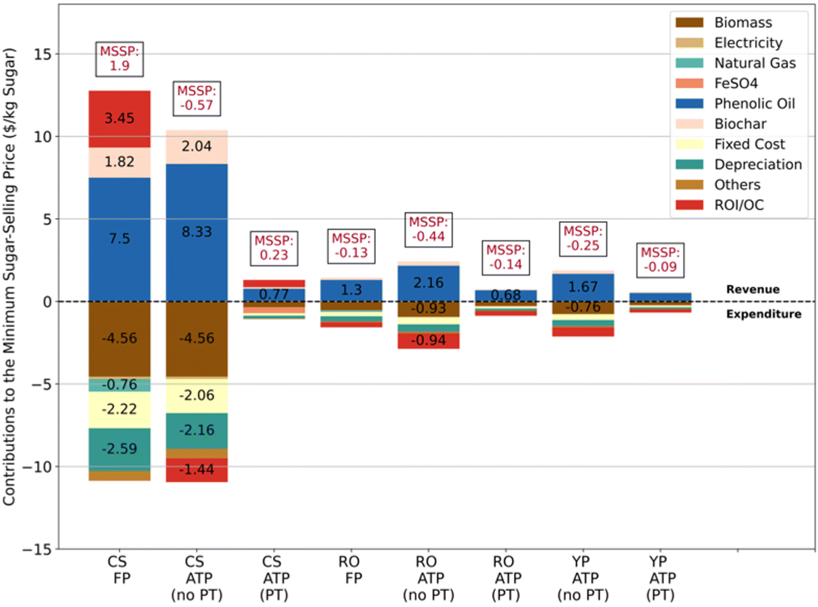
Fig. 3 shows the installed equipment costs associated with the proposed FT and ATP biorefinery systems. In each case, biomass pretreatment and sugar recover are among the most expensive unit operations, accounting for around 56% and 67% of the equipment costs for FP and ATP, respectively. The pyrolysis section of the plant is also a significant capital cost for the FP plant, representing 25% of equipment costs whereas the pyrolysis section is only 10% of equipment costs for the ATP system. The total installed equipment cost are $13 M and $11 M for the FP and ATP systems while the total fixed capital investment (TFCI) are $19 M and $16 M for the FP and ATP systems, respectively. Fig. 4 details the contributions of operating expenses and product revenues on MSSP for the various biorefinery scenarios. The MSSP for a corn stover-based 250 MTPD biorefinery was $1.9 per kg, −$0.57 per kg, and $0.23 per kg for the FP, ATP no PT and ATP PT scenarios, respectively. The MSSP for a red oak-based 250 MTPD was −$0.13 per kg, −$0.44 per kg, and −$0.14 per kg for the FP, ATP no PT and ATP PT scenarios, respectively. The MSSP for a yellow pine-based 250 MTPD was −$0.25 per kg and $0.09 per kg for the ATP no PT and ATP PT scenarios, respectively. With the exception of the FP and ATP PT scenarios for corn stover, MSSP were negative for all other scenarios. A negative MSSP in this study signifies that the plant can attain a positive NPV from revenues generated by selling phenolic oil for production of bio-asphalt and biochar as soil amendment (no carbon removal credits). Thus, the negative ROIs are referred to as opportunity cost (OC) which signifies an excess investment that is not required for the pyrolysis facilities because of high product revenues in Fig. 4. The by-product revenues are more than the expenditures for proper functioning of the plant along with the expected 10% rate of return. ESI Fig. ES3† shows the contributions of different parameters (in $M) towards annual operating costs and revenues, sugar being sold at an average market price over the past 16 years. This gave the understanding how annual sugar and byproduct revenues played a pivotal role in bringing down the MSSPs of the seven (out of eight) plants considered in this study, specifically the ones with FeSO₄ pretreatment, resulting into profitable enterprises, while the corn stover-fed FP plant with no pretreatment resulted in a negative or unprofitable enterprise. Fig. 5 is a sensitivity analysis for the corn stover-based biorefinery scenarios. The three most significant process parameters for the FP (Fig. 5(a)) and ATP no PT (Fig. 5(b)) scenarios were operating hours, phenolic oil price, and biomass price. On the other hand, the same for the ATP PT (Fig. 5(c)) scenario the most significant process parameters were phenolic oil price, operating hours, and FeSO₄ cost.

Fig. 3 Installed equipment costs comparison for a 250-metric ton per day fast pyrolysis (FP) and autothermal pyrolysis (ATP) biorefineries for sugar, phenolic oil, and biochar production.

Fig. 4 Contributions to the minimum sugar selling price for a 250 ton per day fast pyrolysis (FP) and autothermal pyrolysis (ATP) biorefineries producing sugar, phenolic oil, and biochar.

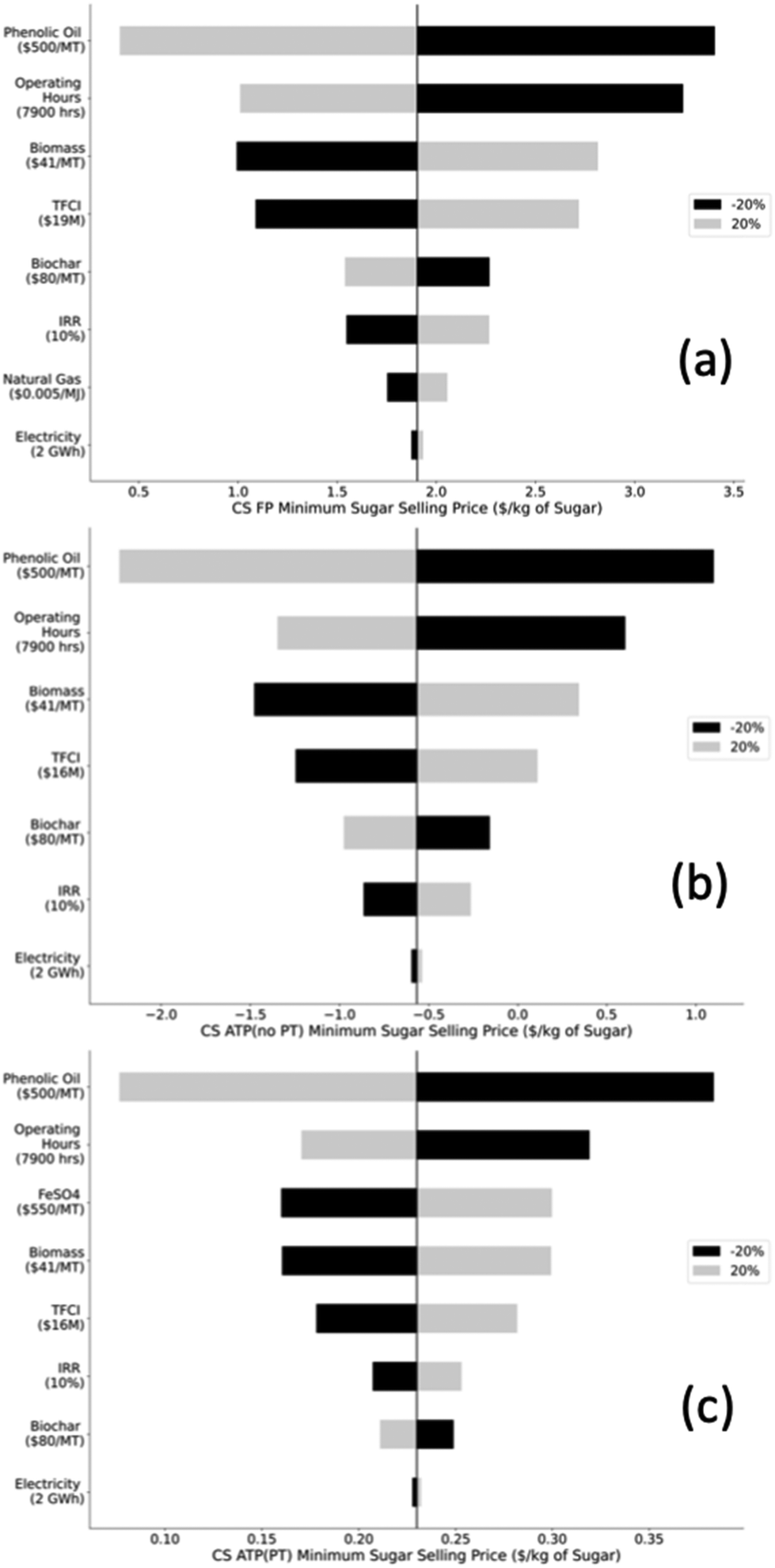Fig. 5 Sensitivity analysis of minimum sugar selling price (MSSP) for corn stover-based biorefineries (a) fast pyrolysis (FP), (b) autothermal pyrolysis (ATP) without pretreatment, and (c) ATP with FeSO₄ pretreatment sugar production with phenolic oil and biochar byproducts. Labels include the baseline values of each parameter.

Fig. ES4–ES6 in the ESI† show the results of TEA sensitivity analysis for red oak feedstock. The three most significant parameters affecting red oak fed FP and ATP (with and without pretreatment) were phenolic oil price, plant operation hours and biomass price. Similar sensitive parameters with same significance were found for yellow pine fed ATP (with and without pretreatment) plants as shown in Fig. ES7 and ES8 in the ESI.† RO ATP(PT) and YP ATP (PT) scenarios showed much lesser sensitivity towards FeSO₄ price because of much reduced pretreatment requirements for red oak and yellow pine compared to corn stover. On the whole, the TEA sensitivity results suggest that process robustness and phenolic oil yield are the key factors for the processes. The TFCI for all scenarios had a lower impact on process profitability than in similar studies. This could be attributed to the low capital intensity and the high product output of the FP and ATP process.

3.2 Life cycle analysis

Fig. 6 illustrates the various contributions to carbon removal/carbon emitted (kg C per kg C in biomass) for different scenarios of 250 MTPD biorefineries investigated in this study. Corn stover-based biorefineries achieved net carbon removal of −0.33, −0.38 and −0.22 kg of C per kg of C in corn stover for the FP, ATP no PT, and ATP PT scenarios, respectively. The red oak-based biorefinery achieved net carbon removal of −0.27, −0.28 and −0.27 kg of C per kg of C in red oak for the FP, ATP no PT and ATP PT scenarios, respectively. The yellow pine-based biorefinery achieved net carbon removal of −0.25 and −0.27 kg of C per kg of C in yellow pine for ATP no PT and ATP PT, respectively.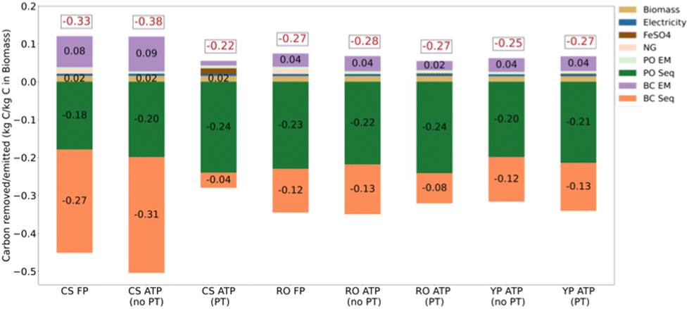

Fig. 6 Carbon removed (negative)/emitted (positive) by the key material and energy resources of a 250 ton per day fast pyrolysis (FP) and autothermal pyrolysis (ATP) biorefinery that produces sugar, phenolic oil, and biochar (EM-emission, PO-phenolic oil, and BC-biochar).

Bioasphalt and biochar both were major contributors towards achieving net carbon removal. Corn stover cultivation, collection, and delivery to the biorefineries contributed around 0.02 kg of C per kg of C in biomass towards positive emissions with similar positive contributions from electricity consumption at the FP and ATP biorefineries. The FP biorefineries had additional carbon emission of around 0.01 kg of C per kg of C in biomass from the use of natural gas (NG), while ATP with FeSO₄ pretreatment accounted for carbon emission of around 0.01 kg of C per kg of C in biomass for corn stover scenario and even lesser for red oak and yellow pine scenarios.

Assuming average biomass production of 5 tons per acre, these results indicate net removal of CO₂ from the atmosphere of around 4.9 tons per acre per year for most of the scenarios evaluated. These CO₂ removal rates are at least 4.5 times greater than can be achieved by other agricultural practices such as no-till agriculture.⁶⁷

Fig. 7 shows the sensitivity analysis of net GHG emissions (kg C per kg C biomass and kg CO_2e per MJ biomass) to changes in key process parameters for corn stover-based biorefineries. Net GHG emissions were about −0.033, 0.038, and −0.022 kg CO_2e per MJ of corn stover processed (upper x-axis values of charts) or −0.33, −0.38, and −0.22 kg C per kg C in corn stover (lower x-axis values of charts) for FP, ATP no PT and ATP PT scenarios, respectively. The two most impactful process variables affecting GHG emissions were the emission factors (EF) of phenolic oil and biochar. In the case of corn stover-based biorefineries, the most significant parameter was biochar EF for both the FP and ATP no PT scenarios followed by EF for phenolic oil. For biorefinery scenarios based on red oak and yellow pine, the most significant parameter was EF for phenolic oil followed by EF for biochar. It should be noted that the EF for phenolic oil is strongly dependent on the energy required to convert it into bio-asphalt, the ratio of phenolic oil-to-petroleum-based asphalt, and the carbon content of the phenolic oil. Similarly, the EF for biochar is affected by the recalcitrance of field-applied biochar, the energy input required to transport and land apply biochar, and the carbon content of biochar, among other factors. The sensitivity analyses for GHG emissions for red oak and yellow pine feedstocks are found in Fig. ES9–ES13 in the ESI.† The scaling factors and their corresponding calculations for converting from kg CO_2e per MJ biomass to kg C per kg C in biomass are also found in the ESI.†

Fig. 7 Sensitivity analysis of GHG emissions and carbon removal for 250 ton per day corn stover-based biorefineries: (a) fast pyrolysis (FP), (b) autothermal pyrolysis (ATP) without pretreatment and (c) ATP with FeSO₄ pretreatment systems for sugar, phenolic oil, and biochar production. Upper x-axis represents GHG emissions in kg CO_2e per MJ of corn stover, and the lower x-axis represents carbon removed in kg C per kg C in corn stover. Labels include the baseline values of each parameter.

3.3 Uncertainty analysis

Uncertainty analysis was performed on historical prices of sugar, biomass, electricity, asphalt, and natural gas found in Fig. 8. The best-fit distributions obtained for sugar, biomass, electricity, asphalt, and natural gas prices were Laplace, Weibull minimum extreme value, Weibull maximum extreme value, normal, and gamma distribution, respectively. Due to insufficient historical data, we assumed the biochar price to have a triangular distribution with a mean price of $80 per MT and a range of $5 to $160 per MT. Similar approach was taken for FeSO₄ price, and we took a price range in between $520 per MT and $650 per MT (as per communication with Crown Technology, Inc. Aug. 29, 2019) with a mean value of $585 MT.

Fig. 8 Historical prices for biomass, sugar, electricity (U.S.), asphalt (U.S.), and natural gas (U.S.).

Fig. 9 shows the best-fit distributions achieved in this analysis. Sugar price has averaged $280 per MT from 1993–2015 while varying between $100 and $700 per MT. The sugar price distribution showed a low probability of negative sugar prices, which was an artifact of the distribution analysis. The probability of biomass prices being between $35 and $55 per MT was very high, with low probability of being as high as $100 per MT. Industrial electricity and natural prices ranged between 4.0 and 7.5 cents per kW per h and $3 and $13 per mcf. It is important to note that electricity and natural gas prices are heavily regulated in the US, so the distributions might not capture the true volatility of price. A limitation of this approach is that market prices are likely to follow trends from the last five years than the previous 10.

Fig. 9 Best-fit probability density distributions for historical biomass, sugar, electricity, asphalt, and natural gas prices.

The probability density functions of the net present values of the sugar FP and ATP biorefineries are shown in Fig. 10. The best scenarios to achieve positive NPV are biorefineries based on pretreated red oak and pretreated yellow pine. On the other hand, corn stover-based biorefineries, although achieving net carbon removal, only attained very low and even negative NPV; thus, the corn stover-based biorefineries are not economically attractive unless a credit is assigned for carbon removal, as subsequently explored for corn stover fed ATP (with and without pretreatment) scenarios. Drops in the market price of asphalt of more than 60% between 2013 and 2017, as shown in Fig. 8, were a key factor contributing to the risk of negative NPV. Low sugar prices and high corn stover costs could similarly contribute to commercialization risk. Moreover, the higher requirement of FeSO₄ for pretreatment of corn stover contributed to comparatively higher costs compared to biorefineries using woody feedstocks (red oak and yellow pine). The lower probabilities were attained primarily in scenarios with much lower yield of sugar and phenolic oil, such as untreated corn stover.

Fig. 10 Probability distributions of the fast pyrolysis (FP) and autothermal pyrolysis (ATP) biorefineries net present values over a period of around 27 years (1994–2021) for production of pyrolytic sugars from corn stover (CS), red oak (RO), yellow pine (YP) with and without biomass pretreatment (PT).

3.4 Comparison with direct air capture system

Table 7 compares negative GHG emissions per energy consumed for 250 MTPD corn stover-biorefineries and a direct air capture (DAC) system⁶⁸ as a function of the source of energy to run the facilities, which includes mixes of renewable energy⁶⁸ and fossil energy sources.⁶⁹ It should be noted that DAC systems, unlike the carbon negative biorefineries proposed here, do not produce energy or chemical products. For comparison purposes, the functional unit for the three systems was converted to 1 MJ of energy input (Table ES4 in the ESI† shows detailed calculations for each system considered). While there are some DAC systems that can rely solely on renewable energy, most emerging systems employ fossil fuels for generation thermal energy to regenerate sorbents and, even to generate some of the power used in the process.⁷⁰ Thus, for this study, we converted the corresponding electricity input of the DAC system to thermal energy and assume world power grid mixtures (see ESI Table ES4†). Red oak and yellow pine scenarios compared to DAC plants with different electrical resources are shown in the ESI (Tables ES6 and ES7†).

Table 7 Comparison of GHG emissions for corn stover (CS) fed fast pyrolysis (FP), autothermal pyrolysis (ATP) (with and without pretreatment) biorefineries and direct air capture (DAC) using different electricity supplies

Electricity supply	CS FP	CS ATP (no PT)	CS ATP (PT)	DAC	References
	(kg CO2e per MJ energy)
Global grid 2030	—	—	—	−0.037	Deutz et al.^68
Global grid 2050	—	—	—	−0.12
Germany grid	—	—	—	0.00016
Renewable grid 1	−3.4	−3.91	−2.31	—
Renewable grid 2	−3.36	−3.9	−2.3	—
Fossil fuel grid 1	−3.25	−3.7	−2.19	—	GREET^69
Fossil fuel grid 2	−3.2	−3.8	−2.21	—
This study	−3.3	−3.85	−2.25	—	Calculated

---

The 250 MTPD corn stover-based FP and ATP no PT biorefineries achieved negative GHG emissions ranging between −3.2 to −3.4 kg CO_2e per MJ and −3.7 to −3.9 kg CO₂ per MJ of energy usage, respectively. An ATP PT biorefinery based on corn stover, while producing more sugar than the biorefineries without biomass pretreatment, did not reach as high of carbon removal ranging only between −2.1 to −2.3 kg CO₂ per MJ of energy usage. This is primarily because this scenario produced a lower yield of biochar with lower carbon content (see Table ES3 in ESI† for calculation details for all three biomass feedstocks).

Considering a world power grid mixture of 2030 and 2050, the DAC plant achieves negative GHG emissions of only −0.04 and −0.12 kg CO_2e per MJ energy, respectively. In fact, DAC plants operating on the German grid would have positive GHG emissions. On an energy basis, the proposed carbon negative biorefineries achieve over an order of magnitude greater carbon removal on an energy consumption basis than DAC plants.

The cost of CO₂ removal is a key metric for assessing the performance of carbon removal technologies. For the ATP and FP biorefineries, this was calculated as the difference between biorefinery operating costs and revenues for phenolic oil, sugars, and biochar (as soil amendment) divided by the net CO₂ removed. Because market prices for commodity products like sugars are high variable over time, the cost of CO₂ removal for a biorefinery are also expected to vary considerably. Fig. 8 plots sugar prices (left axis) and CO₂ removal costs (right axis) over time, from 1994–2022, for corn stover-based biorefineries (FP, ATP no PT, and ATP PT). Over the past decade, FP systems would have had a positive cost for CO₂ removal ranging between $18–$30 per ton of CO₂ removed. However, the ATP scenarios all achieved negative costs for CO₂ removal; that is, the value of pyrolysis products not used as carbon sequestration agents exceeded the operating costs of the biorefinery. A negative cost of CO₂ removal indicates that carbon credits would increase the profitability of a commercially viable process. Corn stover-based biorefineries based on ATP no PT had CO₂ removal costs of −$9 per ton CO₂ to −$17 per ton CO₂ while the ATP PT scenario had CO₂ removal costs of −$9 to −$139 per ton CO₂ over the last decade. In comparison, projected DAC systems have CO₂ removal costs ranging between $100 to $1000 per ton of CO₂ removed.^3,71

The cost of CO₂ removed for 250 MTPD biorefineries based on red oak and yellow pine are shown in ESI Fig. ES14 and ES15.† For the red oak and yellow pine scenarios, since MSSPs were negative in the last decade, the cost of CO₂ removal was also negative, indicating a highly profitable process for carbon removal.

Red oak and yellow pine-fed ATP facilities with pretreatment would generate additional profits from carbon credits at plant capacities smaller than 250 MTPD. ESI Fig. ES16–ES18† investigate the cost of CO₂ removal for corn stover, red oak, and yellow pine fed 50 MTPD FP and ATP plants. It is observed that for corn stover, red oak and yellow pine the cost of CO₂ removal remains positive for FP and ATP without pretreatment scenarios (plant capacity being 50 MTPD). For corn stover FP and ATP no PT scenarios (Fig. ES16†) the costs vary between around $144–$151 per ton CO₂ removed and $81–$87 per ton CO₂ removed in the past decade respectively. The same for red oak (Fig. ES17†) vary between around $11–$78 per ton CO₂ removed and $28.5–$68 per ton CO₂ removed in the past decade respectively. Considering, yellow pine fed ATP (no pretreatment) 50 MTPD plant (Fig. ES18†) the cost of CO₂ removal varies between around $28–$77 per ton CO₂ removed in the past decade. Henceforth, from sustainability point of view, all the five aforesaid scenarios remain highly competitive to a DAC plant (Fig. 11).

Fig. 11 Costs of CO₂ removal and minimum sugar selling prices (MSSP) for corn stover (with and without pretreatment) fed fast pyrolysis (FP) and autothermal pyrolysis (ATP) biorefineries as a function of the historical US sugar price.

On the other hand, all the FeSO₄ pretreated ATP scenarios showed mostly very minimal cost of CO₂ removal, being as low as $19 per ton of CO₂ removed for corn stover scenario (Fig. ES16†), and mostly negative cost of CO₂ removal specially for woody biomass, varying between around −$137 to $9 per ton CO₂ removed for red oak (Fig. ES17†) and −$172 to $2 per ton CO₂ removed for yellow pine (Fig. ES18†) in the past decade. Thus, from both economic (considering present market price of sugar) and environmental point of view, the ATP plants with FeSO₄ pretreatment especially for woody biomass scenarios are both economically and environmentally lucrative at much smaller plant capacity, also while considering the fact that it can obtain additional revenues from carbon price (given a carbon market).

These findings suggest that the ATP system can be operated to maximize product revenues or carbon removal. Thus, public incentives could play an important role in the optimal ATP facility configuration. Furthermore, an ATP system could vary its product distribution in response to market prices and public incentive values.

4 Conclusions

This study investigated the prospects for carbon-negative pyrolysis biorefineries. Biorefineries based on conventional fast pyrolysis (FP) and autothermal pyrolysis (ATP) at a scale of 250 MTPD were compared. Three feedstocks (corn stover, red oak, and yellow pine) were converted into levoglucosan-rich sugar, phenolic oil, and biochar. In three ATP scenarios, the lignocellulosic feedstocks were treated with FeSO₄, which resulted in a higher yield of sugars and phenolic oil, while the feedstocks remain untreated for the FP and ATP (without pretreatment) scenarios leading to smaller yields of both of these products.

All the ATP scenarios achieved significantly lower capital costs compared to FP scenarios. This reflects the relative simplicity of the oxygen-blown pyrolyzer, which does not require equipment like heat exchangers and other ancillary equipment associated with a conventional fast pyrolysis plant. Both FP and ATP plants achieved negative MSSPs for woody (lignin-rich) feedstocks, reflecting the high economic value of phenolic oil for the production of bioasphalt. Corn stover achieved negative MSSP only for ATP without pretreatment of the feedstock. Although pretreatment significantly increased sugar yields, the high ash content of corn stover required large amounts of FeSO₄ for pretreatment, driving up the MSSP to positive values. The high sensitivity of MSSP to ±20% changes in phenolic oil price reflects its high base case value ($500 per ton) compared to other products (sugar and biochar).

Life cycle analyses indicates that all eight plants achieve carbon negative operation, reflecting the large amount of biogenic carbon in the form of bio-asphalt and biochar that are sequestered. This is reflected in the dominance of emission factors for phenolic oil and biochar in the sensitivity analyses for GHG emissions and carbon removal. All scenarios for biorefineries achieved one to two orders of magnitude more carbon removal per unit energy consumption than direct air capture (DAC). This reflects the fact that the pyrolysis biorefineries process energy-rich feedstocks while DAC must capture and concentrate CO₂ from the atmosphere, an extremely energy intensive process requiring large amounts of renewable energy input.

Economic analysis found that the cost of CO₂ removal was negative for 250 MTPD ATP plants with FeSO₄ pretreatment, representing a significant opportunity for generating additional revenue even for carbon markets in which the price is only a few tens of dollars per ton of CO₂ equivalent sequestered. In contrast, the high energy consumption and absence of salable products other than carbon sequestration agent for DAC currently requires carbon prices of hundreds of dollars for a viable business model.

Author contributions

Conceptualization of idea: R. C. B., M. M. W. and A. G., methodology: A. G., M. M. W., and R. C. B., investigation of analysis: A. G., M. M. W., writing the manuscript: A. G., reviewing and editing the manuscript: A. G., M. M. W., and R. C. B., supervision: R. C. B., and M. M. W.

Conflicts of interest

There are no conflicts to declare.

Acknowledgements

This research was funded in part by the American Institute of Chemical Engineers as part of the Department of Energy sponsored RAPID Institute [subcontract #138846]. The authors would like to thank Crown Technology Inc. for providing the FeSO₄ price range.

References

1. J. Tollefson, Nature, 2018, 562, 172–173.
2. IPCC, IPCC says limiting global warming to 1.5 °C will require drastic action, Cambridge University Press, 2021, p. 3949, accessed on 3 November 2021.
3. O. S. Board, E. National Academies of Sciences, Medicine, et al., Climate Change 2021: The Physical Science Basis, 2019.
4. R. Dezember, Preserving trees becomes big business, driven by emissions rules, Wall St. J., 2020, 1–11.
5. D. W. Keith, G. Holmes, D. S. Angelo and K. Heidel, Joule, 2018, 2, 1573–1594.
6. V. Stampi-Bombelli, M. van der Spek and M. Mazzotti, Adsorption, 2020, 26, 1183–1197.
7. S. Fujikawa, R. Selyanchyn and T. Kunitake, Polym. J., 2021, 53, 111–119.
8. R. C. Brown, Processes, 2021, 9, 17.
9. D. L. Sanchez and D. M. Kammen, Nat. Energy, 2016, 1, 1–4.
10. D. A. Laird, R. C. Brown, J. E. Amonette and J. Lehmann, Biofuels, Bioprod. Biorefin., 2009, 3, 547–562.
11. P. Smith, Global Change Biol., 2016, 22, 1315–1324.
12. G. W. Huber and R. C. Brown, Energy Technol., 2017, 5, 5–6.
13. A. Ganguly, I. M. Martin, R. C. Brown and M. M. Wright, ACS Sustainable Chem. Eng., 2020, 8, 16413–16421.
14. K. Wang and R. C. Brown, Fast Pyrolysis of Biomass: Advances in Science and Technology, The Royal Society of Chemistry, 2017.
15. N. S. Hassan, A. A. Jalil, C. N. Hitam, D. V. Vo and W. Nabgan, Environ. Chem. Lett., 2020, 18, 1625–1648.
16. W. Hu, Q. Dang, M. Rover, R. C. Brown and M. M. Wright, Biofuels, 2016, 7, 87–103.
17. M. M. Wright, D. E. Daugaard, J. A. Satrio and R. C. Brown, Fuel, 2010, 89, S2–S10.
18. T. R. Brown, R. Thilakaratne, R. C. Brown and G. Hu, Fuel, 2013, 106, 463–469.
19. T. Bridgwater, Johnson Matthey Technol. Rev., 2018, 62, 118–130.
20. T. Bridgwater, Johnson Matthey Technol. Rev., 2018, 62, 150–160.
21. J. P. Polin, C. A. Peterson, L. E. Whitmer, R. G. Smith and R. C. Brown, Appl. Energy, 2019, 249, 276–285.
22. R. C. Brown, Joule, 2020, 4, 2268–2289.
23. J. P. Polin, H. D. Carr, L. E. Whitmer, R. G. Smith and R. C. Brown, J. Anal. Appl. Pyrolysis, 2019, 143, 104679.
24. R. C. Brown, Energy Fuels, 2020, 35, 987–1010.
25. J. K. Lindstrom, J. Proano-Aviles, P. A. Johnston, C. A. Peterson, J. S. Stansell and R. C. Brown, Green Chem., 2019, 21, 178–186.
26. S. Zhou, D. Mourant, C. Lievens, Y. Wang, C. Z. Li and M. Garcia-Perez, Fuel, 2013, 104, 536–546.
27. D. L. Dalluge, T. Daugaard, P. Johnston, N. Kuzhiyil, M. M. Wright and R. C. Brown, Green Chem., 2014, 16, 4144–4155.
28. S. A. Rollag, J. K. Lindstrom and R. C. Brown, Chem. Eng. J., 2020, 385, 123889.
29. L. Jiang, A. Zheng, Z. Zhao, F. He, H. Li and W. Liu, Bioresour. Technol., 2015, 182, 364–367.
30. D. Liu, X. Yan, M. Si, X. Deng, X. Min, Y. Shi and L. Chai, Environ. Sci. Pollut. Res., 2019, 26, 2761–2770.
31. C. J. Longley and D. P. C. Fung, Adv. Thermochem. Biomass Convers., 1993, 1484–1494.
32. I. Itabaiana Junior, M. Avelar Do Nascimento, R. O. M. A. De Souza, A. Dufour and R. Wojcieszak, Green Chem., 2020, 22, 5859–5880.
33. M. R. Rover, A. Aui, M. M. Wright, R. G. Smith and R. C. Brown, Green Chem., 2019, 21, 5980–5989.
34. W. Li, A. Ghosh, D. Bbosa, R. Brown and M. M. Wright, ACS Sustainable Chem. Eng., 2018, 6, 16515–16524.
35. J. Wang, S. You, Z. Lu, R. Chen and F. Xu, Bioresour. Technol., 2020, 307, 123179.
36. B. T. Brown and R. C. Brown, Biorenewable Resour., 2014, 195–236.
37. Q. Dang, W. Hu, M. Rover, R. C. Brown and M. M. Wright, Biofuels, Bioprod. Biorefin., 2016, 10, 790–803.
38. R. C. Williams, R. C. Brown and S. Tang, Asphalt materials containing bio-oil and methods for production thereof, US Patent 9523003, 2016.
39. M. A. Raouf and C. R. Williams, Road Mater. Pavement Des., 2010, 11, 325–353.
40. J. Peralta, H. M. R. D. Silva, R. C. Williams, M. Rover and A. V. A. Machado, Int. J. Pavement Res. Technol., 2013, 6, 1–10.
41. L. P. Thives and E. Ghisi, Renewable Sustainable Energy Rev., 2017, 72, 473–484.
42. A. Samieadel, K. Schimmel and E. H. Fini, Clean Technol. Environ. Policy, 2018, 20, 191–200.
43. X. Zhou, T. B. Moghaddam, M. Chen, S. Wu, S. Adhikari, S. Xu and C. Yang, ACS Sustainable Chem. Eng., 2020, 8, 14568–14575.
44. D. C. Elliott, H. Wang, M. Rover, L. Whitmer, R. Smith and R. Brown, ACS Sustainable Chem. Eng., 2015, 3, 892–902.
45. J. Haydary, Chemical process design and simulation: Aspen Plus and Aspen Hysys applications, John Wiley & Sons, 2019.
46. P. E. Chris Burk, Chem. Eng. Prog., 2018, 114, 266–269.
47. M. S. Peters and J. I. Peters, Plant design and economics for chemical engineers, McGraw-Hill, New York, (vol. 4). edn., 1959, vol. 5, pp. 27–30.
48. M. Langholtz, B. Stokes and L. Eaton, Ind. Biotechnol., 2016, 12, 282–289.
49. R. M. Campbell, N. M. Anderson, D. E. Daugaard and H. T. Naughton, Appl. Energy, 2018, 230, 330–343.
50. S. Mani, L. G. Tabil and S. Sokhansanj, Biomass Bioenergy, 2004, 27, 339–352.
51. J. J. Jacobson, M. S. Roni, K. G. Cafferty, K. Kenney, E. Searcy and J. Hansen, Feedstock Supply System Design and Analysis, The Feedstock Logistics Design Case for Multiple Conversion Pathways, Idaho National Laboratory, 2014, p. 194.
52. W. Li, Q. Dang, R. Smith, R. C. Brown and M. M. Wright, ACS Sustainable Chem. Eng., 2017, 5, 1528–1537.
53. S. P. Galinato, J. K. Yoder and D. Granatstein, Energy Policy, 2011, 39, 6344–6350.
54. M. Ilbeigi, B. Ashuri and A. Joukar, J. Manage. Eng., 2017, 33, 04016030.
55. Asphalt & Fuel Index, Georgia Department of Transportation, Accessed 2021, URL: https://www.dot.ga.gov/GDOT/pages/AsphaltCementFuelPriceIndex.aspx.
56. Methanol Institute, Methanol price and supply/demand, 2021, https://www.methanol.org/methanol-price-supply-demand/.
57. I. ISO, Environmental management—life cycle assessment—principles and framework, 2006, pp. 235–248.
58. I. O. for Standardization, Environmental management: life cycle assessment; requirements and guidelines, ISO, Geneva, Switzerland, 2006, vol. 14044.
59. ANL, Summary of Expansions and Updates in GREET TM 2 _ 2014 Models, 2014, 5–7.
60. M. Wang, A. Elgowainy, U. Lee, P. Benavides, A. Burnham, H. Cai, Q. Dai, T. Hawkins, J. Kelly, H. Kwon, X. Liu, Z. Lu, L. Ou, P. Sun, O. Winjobi and H. Xu, Summary of Expansions and Updates in GREET 2019, 2019, 24.
61. A. Genovese, A. A. Acquaye, A. Figueroa and S. L. Koh, Omega, 2017, 66, 344–357.
62. Z. Wang, J. B. Dunn, J. Han and M. Q. Wang, Biofuels, Bioprod. Biorefin., 2014, 8, 189–204.
63. A. Tisserant and F. Cherubini, Potentials, limitations, co-benefits, and trade-offs of biochar applications to soils for climate change mitigation, Land, 2019, 8, 179.
64. USDA ERS, Sugar and Sweeteners Yearbook Tables, accessed 2021, URL: https://www.ers.usda.gov/data-products/sugar-and-sweeteners-yearbook-tables/sugar-and-sweeteners-yearbook-tables.
65. R. January, Short-Term Energy Outlook, 1999, pp. 4–6.
66. B. Li, L. Ou, Q. Dang, P. Meyer, S. Jones, R. Brown and M. Wright, Bioresour. Technol., 2015, 196, 49–56.
67. K. Glasener and T. Wagester, Carbon Sequestration in Agricultural and Forest Soils, 2003.
68. S. Deutz and A. Bardow, Nat. Energy, 2021, 6, 203–213.
69. J. Cai, H. Wang, M. Elgowainy and A. Han, Updated greenhouse gas and criteria air pollutant emission factors and their probability distribution functions for electricity generating units, Argonne national lab.(anl), argonne, il (united states), technical report, 2012.
70. M. Fasihi, O. Efimova and C. Breyer, J. Cleaner Prod., 2019, 224, 957–980.
71. J. Meckling and E. Biber, Nat. Commun., 2021, 12, 1–6.

---

Footnote

† Electronic supplementary information (ESI) available. See DOI: https://doi.org/10.1039/d2gc03172h

---