 Open Access Article
 This Open Access Article is licensed under a Creative Commons Attribution-Non Commercial 3.0 Unported Licence
Maintaining the momentum in cryoEM for biological discovery†
Yehuda
Halfon
a,
Louie
Aspinall
a,
Joshua
White
a,
Isobel
Jackson Hirst
b,
Yiheng
Wang
b,
Michele C.
Darrow
cd,
Stephen P.
Muench
 b and
Rebecca F.
Thompson
*a
b and
Rebecca F.
Thompson
*a
aSchool of Molecular and Cellular Biology, Faculty of Biological Sciences & Astbury Centre for Structural and Molecular Biology, University of Leeds, Leeds, LS2 9JT, UK. E-mail: r.f.thompson@leeds.ac.uk
bSchool of Biomedical Sciences, Faculty of Biological Sciences & Astbury Centre for Structural and Molecular Biology, University of Leeds, Leeds, LS2 9JT, UK
cThe Rosalind Franklin Institute, Harwell Campus, Didcot, OX11 0QS, UK
dSPT Labtech Ltd, Melbourn Science Park, Melbourn, SG8 6HB, UK
First published on 15th July 2022
Abstract
Cryo-electron microscopy (cryoEM) has been transformed over the last decade, with continual new hardware and software tools coming online, pushing the boundaries of what is possible and the nature and complexity of projects that can be undertaken. Here we discuss some recent trends and new tools which are creating opportunities to make more effective use of the resources available within facilities (both staff and equipment). We present approaches for the stratification of projects based on risk and known information about the projects, and the impacts this might have on the allocation of microscope time. We show that allocating different resources (microscope time) based on this information can lead to a significant increase in ‘successful’ use of the microscope, and reduce lead time by enabling projects to ‘fail faster’. This model results in more efficient and sustainable cryoEM facility operation.
Introduction
Cryo-electron microscopy (cryoEM) and in particular single particle analysis has gained huge traction in the past decade as a tool for structure determination.1,2 This technique has transformed researchers' ability to gain insight into membrane proteins, heterogeneous complexes and other samples not amenable to other structural techniques such as X-ray crystallography. This surge in activity has been underpinned by wide-spread investment in electron microscopy infrastructure, from instruments based within individual laboratories or institutional research facilities, to large national and international electron microscopy centres.3,4 For the purposes of this manuscript, we will consider a ‘facility’ to be a location with a set of cryoEM hardware, dedicated staff and a remit to support the research of more than one research group. The investment in cryoEM facilities across the globe spans beyond the microscopes and associated hardware (e.g., direct electron detectors), into ancillary laboratory space including equipment for sample preparation, computing hardware to process and store the data, specialised rooms and buildings to house the equipment, and, of course, expert staff to manage, maintain and operate equipment. To support end-to-end structure determination and model/map interpretation, the full pipeline of infrastructure is required, although this does not necessarily need to be co-located in one facility or even country.There are a diverse set of cryoEM facilities globally, with differing microscope hardware, funding models, project mixes, user communities and core aims. All of these factors influence how a facility infrastructure should be resourced and structured to support its user communities. The operational model, data collection strategies employed and wider resources including staff and computing should be structured to match the aims of the projects within the facility.
The single particle structure determination pathway is often presented as a linear, stepwise process, although those with cryoEM experience will likely recognise the need for multiple retrograde steps in order to progress through the stages (Fig. 1). At the facility level, the efficiency of and support available for each step in the process should be considered and optimised to maximise the output from the most expensive (per day) of these steps: data acquisition.
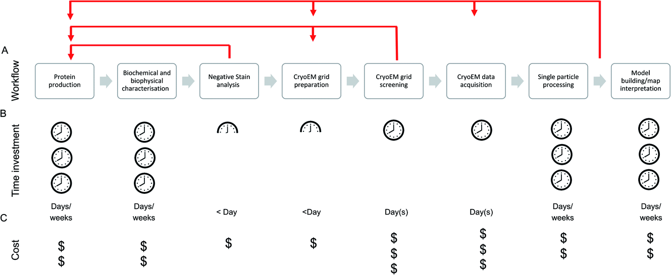 | ||
| Fig. 1 (A) Example of a single particle cryoEM pipeline showing a linear progression through the stages in blue arrows, with common retrograde steps shown in red. (B) Average researcher time investment needed at each stage of the process. (C) Direct costs associated with each stage (cost of machine time, consumables). Time and cost are both intertwined and the actual costs borne by a project also vary based on the financial model of a facility, for example some centres receive core funding so instrument access is free at point of access. | ||
Due to the cost per day, much emphasis is placed (including in this manuscript) on efficiency and throughput at the cryoEM data acquisition stage, conducted on the microscope. While this is of relevance (whether the cost is directly incurred by the user or taken on through core/centralised funding) when accessing high-end cryoEM instrumentation, time is now generally not the most common ‘bottleneck’ in our view – although efficient use of microscope resources is still vital given the overall demand for high-end cryoEM instrument access.
Sample preparation remains a major challenge for many cryoEM projects. For the majority of single particle cryoEM researchers, the main approach used for cryoEM specimen preparation is filter paper-based blotting followed by plunging into a cryogen such as liquid ethane, as first pioneered by Jaques Dubochet and colleagues.5 Whilst countless high-resolution structures have and still are being obtained from grids prepared using blotting-based techniques,6,7 for many samples the production and/or reproduction of good quality grids using this approach is challenging. Research into the causes of variation in grid quality indicates that issues such as protein aggregation, denaturation, preferred particle orientation, subunit dissociation and particle concentration are being caused or exacerbated by interactions between the sample and the air–water interface or the sample and the filter paper.8–11 This has led to the development of alternatives to blotting-based approaches that aim to minimise uncontrolled sample interactions and improve reproducibility.12–15 Most of these technologies do this by generating small droplets (using a variety of methods) which are deposited on the grid en route to the cryogen. By removing the blotting step, decreasing the time between sample deposition and vitrification, and automating more of the process (including sample deposition), some of the aforementioned issues can be reduced and even completely avoided for otherwise difficult samples.16–18 Although this new generation of technology increases the range of grid preparation tools available, we still have a poor understanding of many of the fundamental processes that occur during grid preparation which make some proteins more amenable than others to downstream structural studies. The process of making cryoEM grids is very quick in the context of the structure determination pipeline, however screening and working iteratively through the process to find a grid with suitable characteristics for data collection can be a major hurdle.
Grid screening to assess suitability for data acquisition typically involves a manual inspection of the particle distribution and ice thickness, and/or the acquisition and processing of a small test dataset. The process of screening can be time consuming and subjective, especially for those new to the field, but even highly experienced individuals are not always able to accurately predict the subsequent outcome of a data collection. Once a suitable grid is obtained, a single particle data acquisition session can be scheduled (or take place immediately). The microscope, detector, collection parameters (dose rate, total dose, magnification) and length of the collection can be chosen to try and match the needs of the project.
After data acquisition, single particle image processing approaches are used to reconstruct a three-dimensional (3D) EM density map of the specimen which can then be subject to model building and further interpretation. Leading software packages for single particle reconstruction such as RELION and cryoSPARC19,20 offer a pipelined approach to this workflow. Graphical user interfaces present users with a list of jobs ordered according to their respective position in the pipeline, with default parameters enabling non-expert users to complete the basic workflow and achieve informative results. However, most projects presently require an iterative approach in which sections of the pipeline, such as 3D classification, are revisited several times, with different parameters and intentions, to gain a better understanding of a dataset and its heterogeneity. Thus, processing of single particle datasets demands a significant amount of computational resources and hands-on computational time invested by the user, both of which are potential bottlenecks in progressing from sample to structure.
Notably, the steps at the beginning of this workflow – pre-processing of images including motion correction and CTF estimation – are routinely performed on-the-fly,21 enabling quality assessment of the data coming from the microscope in real-time. More recently, the application of machine learning software has facilitated the automation of steps that traditionally required extensive user input. Software packages such as crYOLO22 and TOPAZ23 permit accurate, unsupervised particle picking through the use of pre-trained, convolutional neural-network (CNN) models. As such, the identification of particles in micrographs can be incorporated into a fully automated processing pipeline. Extraction of these particles is then followed by 2D classification after which 2D class averages containing recognisable protein features must be identified and carried forwards, to select ‘good’ particles and discard those that are sub-optimal. This selection is traditionally subjective and carried out manually by the user. However, recent work has demonstrated the utility of a CNN model for unsupervised 2D class selection, overcoming subjectivity and expanding the section of the single particle workflow that is amenable to automation.24 For example, the Schemes framework within RELION 4.0 permits robust unsupervised processing up to, and including, the generation of a series of initial models, significantly reducing the time between image acquisition and 3D reconstruction.
In this article we will discuss past trends in single particle data acquisition and their impact on the present and future operations of cryoEM research facilities, with a focus on how these might influence the efficiency and throughput of structure determination by cryoEM. We will discuss the challenges and opportunities that these emerging technologies present and propose guiding principles for efficient facility operation going forward.
Results and discussion
CryoEM screening and data acquisition
It is well documented that there has been a substantial growth in the quantity of cryoEM structures being solved, and a trend of improving resolution over the past decade. Here we looked to interpret these trends in the context of microscope hardware and direct electron detectors used. The rapid growth in cryoEM structure determination has been driven by the use of Titan Krios microscopes; since 2016 the total number of structures deposited using Titan Krios microscopes manufactured by FEI (now Thermo Fisher Scientific (TFS)) has outnumbered every other microscope type (Fig. 2A). Historically the predominantly used direct electron detector was the K2, only surpassed now by use of the K3, both manufactured by Gatan (Fig. 2B and C). As EMDB submissions tend to coincide with the final stages of a project (usually upon publication), it is likely that these statistics lag 1–2 years behind data being collected today. We see long ‘tails’ as use of a particular detector drops off, as data sometimes collected several years ago is further analysed or reanalysed and published, the Falcon 2 being a good example of this.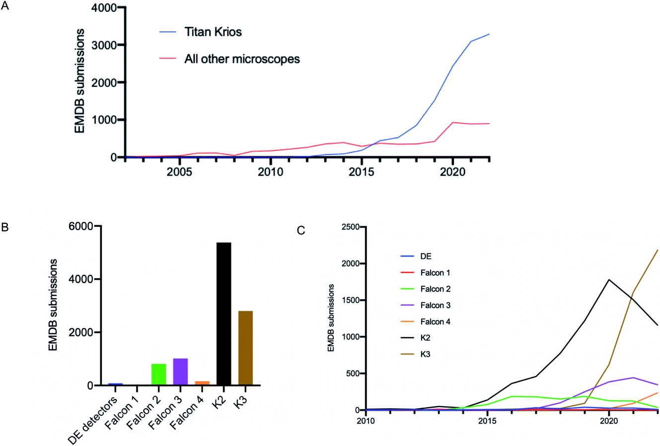 | ||
| Fig. 2 Analysis of single particle EMDB submissions to reveal trends in microscope and detector usage. 2022 data has been adjusted to predicted full year values on a pro rata basis projecting a year end total, to assist identification of trends. (A) Single particle EMDB submissions using specific microscope technology over time. (B) Total single particle EMDB submissions making use of specific direct electron detectors. (C) Use of direct electron detector models for single particle data acquisition over time. | ||
The first electron microscopy data bank (EMDB) deposition for a single particle cryoEM structure from a Titan Krios microscope with a direct electron detector was in 2013 (EMD-2238), where data was collected on a Falcon I. In the >9 years since, direct electron detector technology has evolved considerably. All three of the major direct electron detector manufacturers (Direct Electron, Gatan, and TFS) have released multiple iterations of detector in this time. Looking across all submissions to the EMDB, we see the average resolution reported for single particle structures improving as new iterations of detector technology are released (Fig. 3). This trend is particularly linear for the Thermo Fisher Scientific Falcon series of direct electron detectors (Fig. 3A). As new detector technology comes online, these typically come with an uplift in the throughput of image acquisition as well as an improvement in the quality of the images obtained (sometimes presented through DQE measurements) (ESI Table S1†).31–40 This improvement in detector quality has, alongside improvements in protein biochemistry, cryoEM sample preparation, and image processing methods, led to an average improvement in the resolution of cryoEM structures. However, we and others have noted that single particle data collected on the same sample and sometimes the same grid using different camera technology results in significant differences in resolution and so detectors are likely to be a key factor.
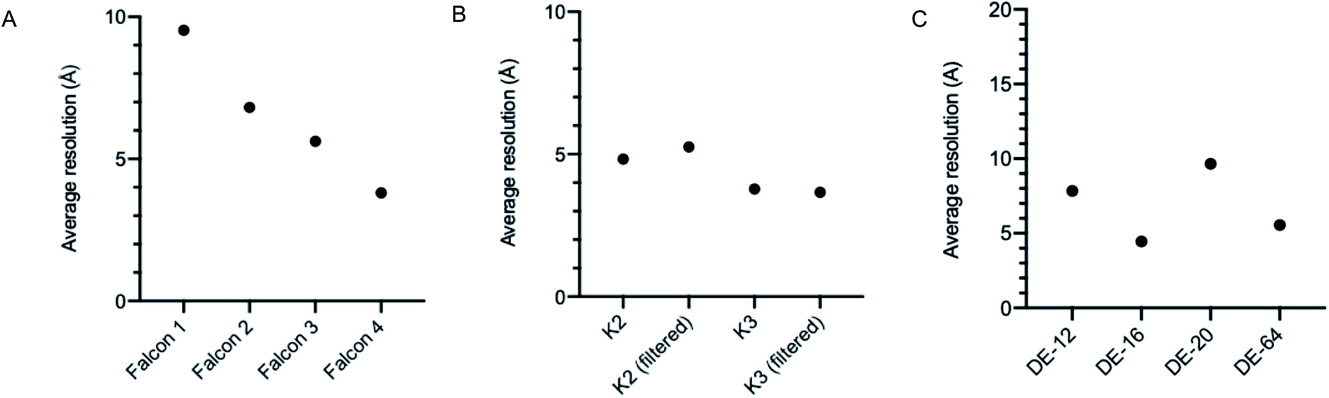 | ||
| Fig. 3 Average resolution for single particle EMDB submissions related to the direct electron detector used, taking no account of sample, microscope or other variables. (A) TFS cameras Falcon 1-4. (B) Gatan cameras K2, K3 filtered and unfilterd. (C) Direct electron cameras DE-12, DE-16, DE-20, DE-64. | ||
Alongside improvements in detector speed, fringe free illumination (FFI) and aberration free image shift collection (AFIS) have been introduced and implemented to further increase the speed of collection. AFIS enables the use of beam-image shift for collection of single particle data, whilst preventing consequential coma and astigmatism that would otherwise reduce data quality. This is achieved by compensatory adjustments to the deflection coils and objective stigmator when performing beam-image shift at different distances. Collecting with AFIS is typically performed within 6–12 μm (ref. 25) of the stage location and increases the throughput substantially by reducing the number of stage movements required. Each stage move takes time, alongside the associated stage settling wait time, and so reducing the number of stage movements increases the speed of a typical acquisition.
The diameter of illuminated area determines how many images can be collected per hole while ensuring each acquisition area is not double exposed. Typically, when the condenser 2 aperture is imaged out-of-focus (while the sample is in focus), wave interference at the edge of the condenser beam appears as Fresnel fringes. As a result a larger illuminated area must be used to exclude these fringes from the image. FFI involves an adjustment to the microscope to minimise the presence of Fresnel fringes in the recorded image at a specific magnification. With FFI implemented, both the C2 aperture and the sample will be in focus and no, or very few, Fresnel fringes will be visible in the recorded image. This allows for a reduction of the beam size and more images acquired from a single hole, againallowing more images to be acquired per stage move (Fig. 4).
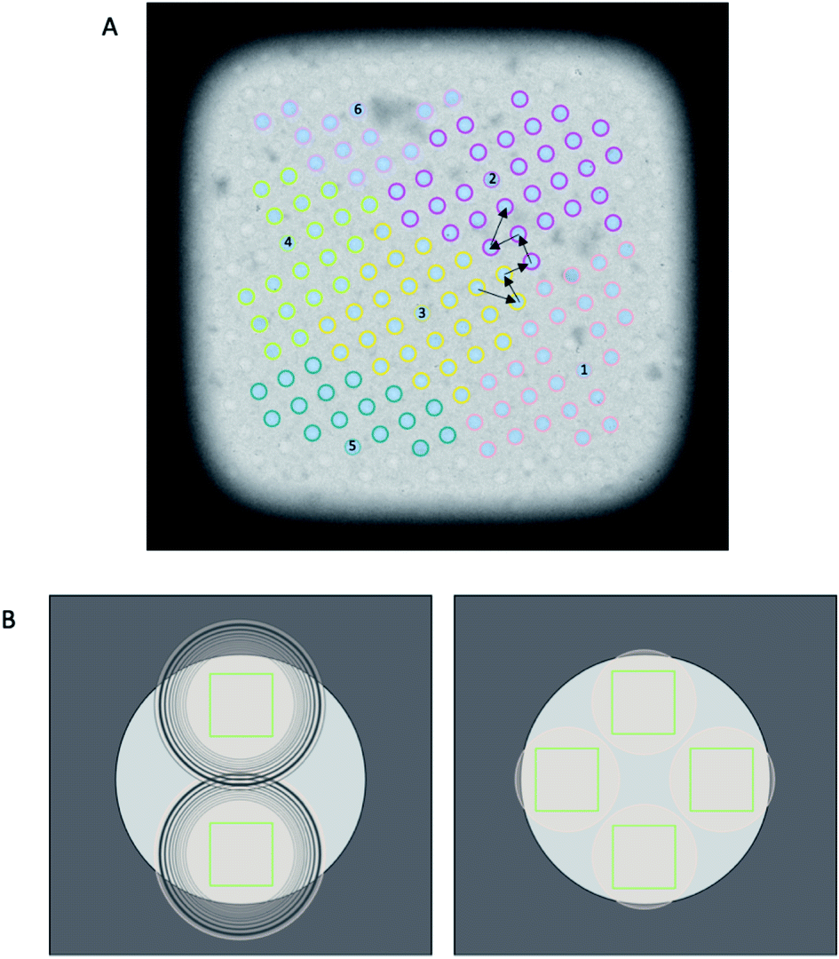 | ||
| Fig. 4 Impact of acquisition schemes of AFIS and FFI. (A) A typical collection scheme is shown with and without AFIS. Without AFIS, the stage moves to each hole individually. Black arrows are shown to indicate this stage movement. With AFIS, the stage centres on one hole, and beam-image shift is used to acquire images in adjacent holes without moving the stage. The different AFIS groups are coloured uniquely, with the central hole numbered. (B) A typical hole template is shown without (left) and with (right) fringe-free illumination. The absence of Fresnel fringes means that a greater number of acquisitions is possible within the same space. | ||
These advances mean that on average, the number of images collected per hour in a single particle data acquisition session is far higher than in previous years. However, disentangling trends in average dataset size is challenging because EMDB submissions can contain a mixture of micrographs and particle stacks, amongst other data and each EMDB entry can be associated with multiple EMPIAR entries and vice versa. These complications make it difficult to assess the relationship between the amount of data collected to yield each EMDB submission.
Implications for ‘standard’ single particle pipelines
To achieve a high level of confidence that a cryoEM grid is suitable for high-resolution imaging, the screening step is essential. Two main factors are assessed during screening: (1) sample biochemistry and suitability; (2) grid and ice quality. While a relatively well-defined process currently exists for assessing sample biochemistry and suitability (purification techniques, activity assays, negative stain EM), this aspect of grid screening is often not optimised. Sample homogeneity, stability during the freezing process, and interaction with the substrate or the air–water-interface can all create issues which are only found during cryoEM grid screening.Both the specimen preparation and microscope hardware can influence the time taken and success of the screening step. Newer specimen preparation technologies provide a view of the grid from the freezing process which can be used to judge the quality of the grid and ice without loading into a microscope.15,27–30 Screening for appropriate ice thickness, and particle concentration and distribution can be done manually. However this is dependent on microscope operator experience, and is always a subjective judgement. Additionally some issues, such as preferred orientation or partial denaturation, will only become obvious after processing at least a small dataset.
In the majority of facilities, the ‘working day’ (for the purposes of this paper we consider this an 8 h window) is ∼9am–5pm, where the majority of staff are on site. Automated data collection (which can run 24 h per day) is then used to collect data when staff are offsite. Due to these standard working patterns, the majority of facilities scheduling occurs in 24 hour time blocks. Historically this would have meant 24 h collection on a single project. However, recently developed tools in programs such as EPU and SerialEM have opened possibilities to collect multiple datasets on different grids while the microscope is unattended. This enables users to collect datasets more tailored to the needs of the project and based on their target resolution or aim of the project, whilst also utilising the imaging resources of the facility better, especially over weekends or public holidays.
Multi-grid imaging also enables a more efficient collection of small ‘proof-of-concept’ datasets, typically 0.25–4 hours, for the purpose of providing better understanding of the condition of the grid and indication of whether a longer data acquisition is required and/or warranted. This style of data collection is necessary because it is difficult to predict through manual assessment of the micrographs alone if the complete complex is present, if factors that may impact structure determination such as preferred orientation are present, and if the desired resolution will be obtainable from the grids. Once a suitable small-scale data collection has been completed and processed, the relationship between the resolution of a 3D reconstruction and the number of contributing particles can be assessed. By running a series of 3D refinements on random subsets of particles from the particle stack, where the subset size is doubled after each refinement, a B-factor plot (or Rosenthal–Henderson plot)26 can be generated.
With tools that remove the current confinement to 24 h ‘blocks’ and an increasing acknowledgement that manual screening is unlikely to confidently predict success at the data acquisition stage, there is an opportunity to change the standard pipelines for cryoEM data acquisition. A workflow based on manual assessment of micrographs (Fig. 5A) with a single ‘gate’ determining if the project should proceed to the next stage is likely to be replaced by a multi-step process (Fig. 5B) that makes use of short collections and more robust metrics of quality to more confidently predict success of data acquisition sessions.
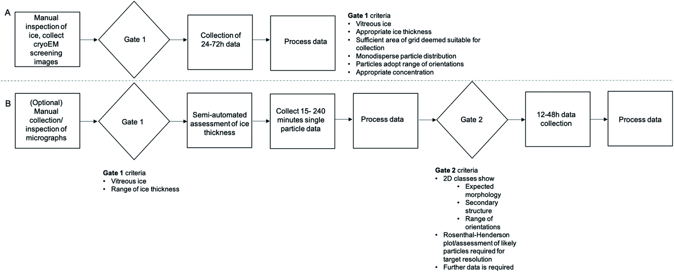 | ||
| Fig. 5 Manual vs. automated approaches to cryoEM screening and data analysis. (A) ‘Standard’ pipeline from cryoEM screening relying on manual inspection of micrographs and particle distributions. (B) Using automated or semi-automated tools to collect and process a small dataset before going on to a larger data collection session if warranted. The pathway in (B) identifies failure more quickly without incurring as many resource or opportunity costs. | ||
Allocation of microscope resources based on project risk profile
We have conducted an analysis to show the theoretical gains that can be made by allocating different projects varying microscope resources, based on the properties of the project. In this analysis we have compared a ‘fixed’ pipeline (Fig. 6A) against ‘probability based’ pipelines (Fig. 6B–E). For each pipeline, we have assigned a global chance of probability for each attempt at the pipeline, and for the variable pipelines a percentage of projects that fall into each category. These numbers are based on qualitative data from our cryoEM facility, but in reality the nature and mix of projects between facilities and even in each facility over time will always change. We see that the situations presented reflect a realistic mix of projects and an example framework which can be altered to suit different project and hardware mixes within other facilities.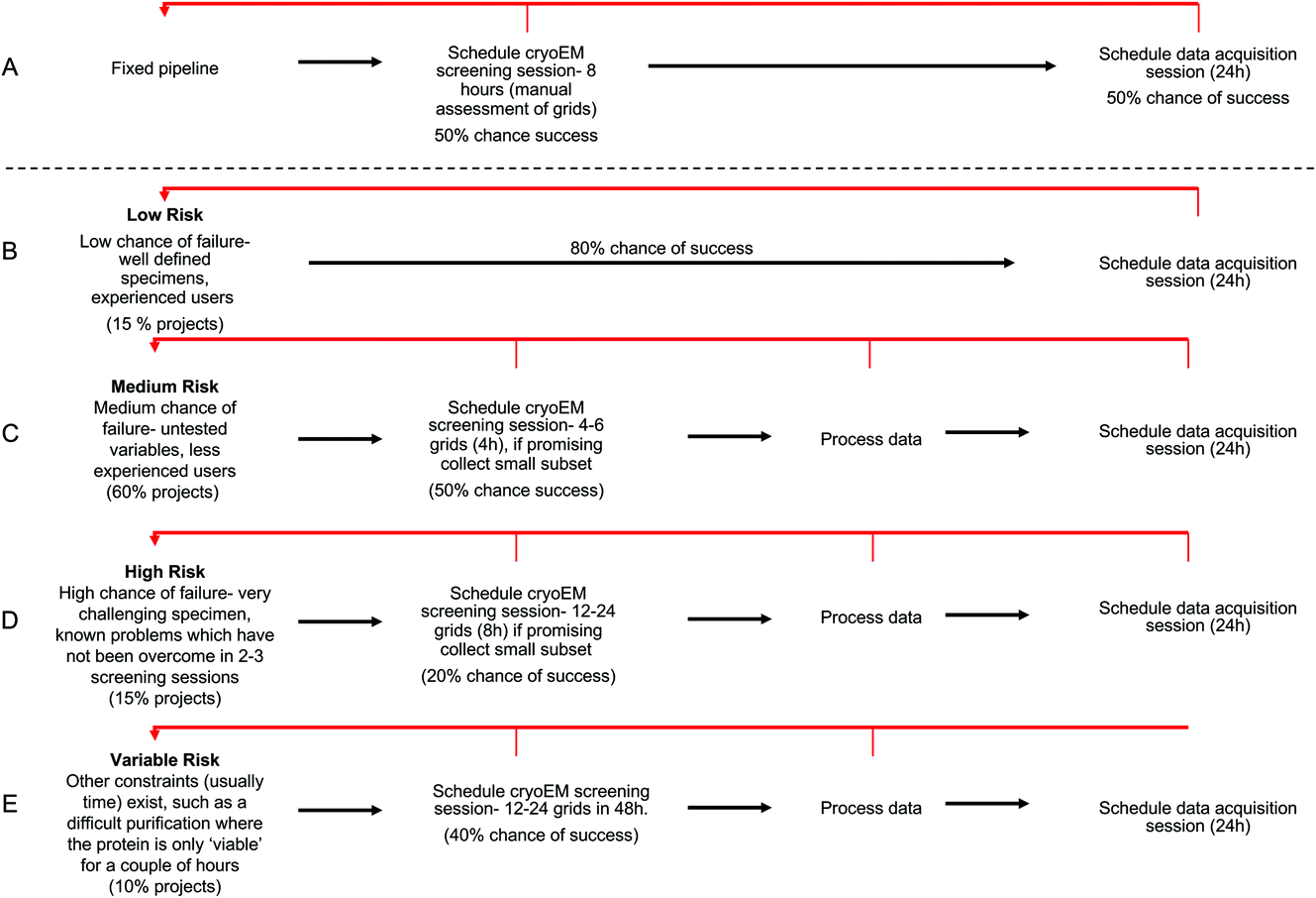 | ||
| Fig. 6 Examples of project categorisation and downstream suggested workflow with chance of success expressed as a % (data shown in ESI Table S2†). Retrograde steps are shown in red arrows. (A) Fixed pipeline, all projects receive 8 h of screening time followed by 24 h of data collection if manual inspection identifies a good grid. (B–E) Stratified approach to resources applied to each project. (B) Low chance of failure (e.g., well characterised icosohedral virus), project is immediately allocated 24 h collection. (C) Medium chance of failure, 4 h screening is allocated with a collection session scheduled if the small processed dataset confirms grid is suitable. (D) High chance of failure, 8 h screening is allocated with a collection session scheduled if the small processed dataset confirms grid is suitable. (E) Variable chance of failure or where there are other time restrictions applied, 24 h is allocated in the first instance with further collection scheduled where initial processing confirms suitability. | ||
The definition of ‘success’ varies largely on a project by project basis, but essentially a ‘successful’ progression through the pipeline means no requirement for a retrograde step (i.e. the quality of data obtained was sufficient to answer the question in hand). For example, for ‘successful’ screening; in the fixed pipeline, success might look like monodisperse particles at a good concentration with vitreous ice. For a ‘medium’ risk project, success would be defined as 2D classes from a pilot collection showing secondary structure detail, a complete complex and a range of views.
In the fixed pipeline, all projects are assigned the same microscope resources initially – an 8 h manual screening session. After this screening, if manual inspection of the micrographs looks promising (vitreous ice, good particle distribution as judged by eye) a 24 h collection is scheduled. For variable pipelines, we have provided examples of ‘low’, ‘medium’, ‘high’, and ‘variable’ risk projects. A ‘low’ risk project would involve a well defined, homogeneous, specimen in the hands of an experienced researcher. Examples might include icosohedral viruses. We assigned these projects an 80% chance of success and estimate that 15% of projects fall into this category. ‘Medium’ risk projects form the majority of projects seen in our facility, at 60% of projects. These are projects where there is a 50/50 chance the grids will be optimal during the screening session, either because the sample requires optimisation (biochemistry or cryoEM grid preparation) or because the user is developing their cryoEM skills, or both. Samples may include those not previously imaged by cryoEM but where preliminary data from negative stain looks promising. ‘High’ risk projects are those where there are obvious challenges with the sample (for example, a medium risk project that has had 3+ imaging sessions would move into the high-risk category).
During standard workflows, there is usually a time gap between when grids are made and then when they are imaged. For the majority of projects this is acceptable or workable, but there are specific cases where microscope time may need to be scheduled to allow immediate feedback about the grids to allow more grids to be made. An example might include a challenging protein purification where the protein cannot be frozen or stored. We have termed these ‘variable’ probability.
Here we have proposed that each categorised ‘risk’ of project is assigned different up-front microscope time based on the risk profile of the project. For example, low risk projects are directed immediately to a 24 h collection session, as the grids are likely to be suitable for collection. Medium risk projects are initially assigned 4 h screening, high risk projects 8 h of screening and variable risk projects 48 h microscope time. Within this initial session, users would be expected to collect a small subset of data (even 20 minutes can be highly informative) on their most promising grid(s) and then process this data to yield at least 2D class averages. Only if these show evidence of a promising structure (secondary structure detail, range of views, whole complex present) will a 24 h data collection session be allocated.
The full data calculations are shown in ESI Table S2,† and are based on the workflows and % chance of success shown in Fig. 6. This shows that if a fixed pipeline is used for 100 projects, 2000 hours of microscope time is required, of which 1200 h is within ‘working hours’ while 800 h is out of hours. If we compare this to the alternative approach of allocating resources based on project risk, for the mix of projects shown here, for 100 projects, 1656 h of microscope time is required, of which 570 hours are ‘working hours’ and 1086 are ‘out of hours’.
Overall, taking a risk based approach to projects means that for 100 projects with the same overall probability of success (0.5 for fixed pipeline, 0.51 for variable pipeline), less microscope time is used overall, reducing demand for microscope time and decreasing wait times between sessions. Significantly, the amount of ‘working hours’ required is also reduced in the risk-based approach. Given that scheduling of microscope time is typically based around when human operators are present to input into decision making, this also helps to reduce the wait time for microscopes. In the risk-based approach, more microscope hours lead to a ‘successful’ outcome and fewer microscope hours are wasted (or ‘failed’) compared with the fixed pipeline.
While the theoretical argument for the risk based approach is clearly compelling, there are barriers to its efficient implementation. The project mix and resources available, along with the culture of the workplace relating to out of hours and weekend working will all vary how the framework is stratified and the resulting potential benefits. Splitting projects into risk bins may be extremely challenging and require the active and willing participation and cooperation of the user community. For the system to work optimally, facility staff should have good working knowledge of projects coming through the facility and a user community who understand the population level benefits of engaging with the system (e.g. reduced time between requested microscope sessions) and providing information to enable the best possible characterisation of the projects. With this in place, project categorisation should always be considered dynamically. Even with these considerations in mind, we feel the majority of facilities will likely benefit from project and resource allocation based on risk, compared with a ‘one-size fits all’ approach.
Another barrier to implementation of this model is facility staff time. Shorter microscope sessions may require loading of the microscope more frequently, and a larger number of shorter collections increases the amount of staff support required. One mechanism of tackling this is increasing users’ independence on the microscope; a second is increasing staffing within the facility. The model and financial constraints of each facility will impact which routes are taken to deliver facility operations.
In our experience, long waits for microscope time (especially screening time) are one of the biggest concerns for a cryoEM researcher, as it can be difficult to make any progress on the project when the outcome from initial screening is not yet known. Generally, microscope time ‘little and often’ is considered to be more useful than longer sessions with large wait times in between. Focusing facility operations to keep the time users wait between sessions to a minimum allows us to meet this need of the cryoEM community. Another benefit of this system is it allows a larger amount of microscope time to be allocated up front to the projects that will really stand to benefit, maximising chances of successful structure determination for these more challenging systems.
For the purposes of this analysis we have allocated 24 h to each ‘data collection’ session. In reality, as discussed above 24 h may not be the optimal amount of time to collect data; for some projects it may be far too much and for some projects not enough. It is highly likely that the model presented here for a risk based approach to allocation of resources can and should be extended out to include a variable amount of data collection time based on the known properties of the macromolecule and the desired outcome for the project. This would likely further improve the efficiency of the framework.
Many institutions worldwide are looking to improve their environmental sustainability, and often have ‘net zero’ emission targets. Operating hardware such as electron microscopes has a carbon cost, but the data generated may have a significant and longer lasting carbon footprint. Data generated must be processed and then stored; many funders then stipulate that these data must be stored past the end of the grant, for up to 10 years. Collecting more data than required has not only a microscope time ‘cost’ associated with it but also a carbon cost, which scales according to the amount of data. Larger datasets are more computationally expensive to process, and store. A final benefit of the risk-based framework proposed here is that overall less ‘bad’ data will be produced, which will not require processing and storage.
Conclusion
To industrial researchers, the framework presented may sound familiar as there are well-studied systems in place to identify priorities and risks, and optimise business resources to meet these needs. When these systems are well-defined and well-used, they can create optimal workflows with clear ‘stages’ and ‘stage-gates’ to help both users and facility staff to understand what criteria to assess their project against, when to follow a certain workflow or when to stop collecting data. These systems, if thoughtfully applied to the cryoEM facility, could substantially shift the way we implement single particle cryoEM data collection beyond the standard 24 hour allocation block and to improve the overall efficiency of microscope time, maximising biological discovery.A vision for a future cryoEM facility would integrate data from across the pipeline, from biochemical and biophysical analysis, cryoEM specimen preparation and on-the-fly analysis of micrographs into 2D and 3D data, as data are collected. These data could then be used to make dynamic, on-the-fly decisions about progressing or halting data acquisition, automatically moving onto the next sample.
To work towards an idealised vision and maximum output for imaging biological specimens, much work is still outstanding both on the specimen preparation and image processing pipeline elements to support new approaches in microscope scheduling. Many variables impacting the success of specimen preparation are still not understood requiring cryoEM grids to be empirically tested which can take valuable time and resources. Work to better understand the factors influencing specimen preparation and next generation specimen preparation devices may transform this portion of the pipeline. During microscope data collection sessions, machine learning approaches may help users to identify optimal areas for data acquisition with minimal or no human intervention. On the image processing side, on-the-fly image processing, automation, and the implementation of deep learning mean that assessing the quality of a sample and its amenability to high-resolution structure determination has never been faster and will improve further in the future. Coupled with new automated, optimised acquisition capabilities across grids, this offers new opportunities to the user, such as investigating the effect of buffer conditions on the compositional heterogeneity of a sample, or assessing the influence of additives (such as surfactants and detergents) in improving particle behaviours (e.g. preferred orientation) all within a single session.
Only when information is integrated across the cryoEM pipeline, supported by fast and accurate image processing, will we be able to most efficiently distribute time on high-end cryoEM infrastructure. While this future is not quite here, recent exciting advances have and will continue to challenge facility managers to consider how best to organise the distribution of resources within their facility to maximise biological discovery.
Experimental
EMDB analysis
Data was downloaded from the EMDB and EMPIAR on 22nd May 2022. Only single particle data filtered according to the field structure_determination_method = single particle was collected. The field microscope_name was altered to ensure all Titan Krios microscopes were included (both FEI and TFS manufacturer titles). In film_detector_model again similar categories were collated. Any entries that used multiple detectors associated with 1 EMDB entry were excluded.Author contributions
RT, SPM and MD conceptualised and supervised the project. YH, LA, JW, IH and YW curated and analysed data. All authors contributed to writing and editing the manuscript.Conflicts of interest
MCD is employed by SPT Labtech and works on the chameleon specimen preparation system.Acknowledgements
We thank Neil Fonseca and Andrii Ludin from the EMDB for their support with EMDB and EMPIAR data acquisition.References
- W. Kühlbrandt, The Resolution Revolution, Science, 2014, 343(6178), 1443–1444 CrossRef.
- M. A. Cianfrocco and E. H. Kellogg, What Could Go Wrong? A Practical Guide to Single-Particle Cryo-EM: From Biochemistry to Atomic Models, J. Chem. Inf. Model., 2020, 60(5), 2458–2469 CrossRef CAS.
- B. Alewijnse, et al., Best practices for managing large CryoEM facilities, J. Struct. Biol., 2017, 199(3), 225–236 CrossRef.
- K. Sader, et al., Industrial cryo-EM facility setup and management, Acta Crystallogr., Sect. D: Struct. Biol., 2020, 76(4), 313–325 CrossRef CAS PubMed.
- J. Dubochet, et al., Cryo-electron microscopy of vitrified specimens, Q. Rev. Biophys., 1988, 21(2), 129–228 CrossRef CAS PubMed.
- Y. Cheng, Single-Particle Cryo-EM at Crystallographic Resolution, Cell, 2015, 161(3), 450–457 CrossRef CAS.
- T. Nakane, et al., Single-particle cryo-EM at atomic resolution, Nature, 2020, 587(7832), 152–156 CrossRef CAS PubMed.
- A. J. Noble, et al., Routine single particle CryoEM sample and grid characterization by tomography, Elife, 2018, 7, e34257 CrossRef PubMed.
- D. Lyumkis, Challenges and opportunities in cryo-EM single-particle analysis, J. Biol. Chem., 2019, 294(13), 5181–5197 CrossRef CAS PubMed.
- R. M. Glaeser and B.-G. Han, Opinion: hazards faced by macromolecules when confined to thin aqueous films, Biophys. Rep., 2017, 3(1–3), 1–7 CAS.
- E. D'Imprima, et al., Protein denaturation at the air–water interface and how to prevent it, eLife, 2019, 8, e42747 CrossRef.
- Y. Z. Tan and J. L. Rubinstein, Through-grid wicking enables high-speed cryoEM specimen preparation, Acta Crystallogr., Sect. D: Struct. Biol., 2020, 76(11), 1092–1103 CrossRef CAS PubMed.
- D. Kontziampasis, et al., A cryo-EM grid preparation device for time-resolved structural studies, IUCrJ, 2019, 6(6), 1024–1031 CrossRef CAS PubMed.
- H. D. White, et al., A second generation apparatus for time-resolved electron cryo-microscopy using stepper motors and electrospray, J. Struct. Biol., 2003, 144(1–2), 246–252 CrossRef CAS PubMed.
- M. C. Darrow, et al., Chameleon: Next Generation Sample Preparation for CryoEM based on Spotiton, Microsc. Microanal., 2019, 25(S2), 994–995 CrossRef.
- T. S. Levitz, et al., Effects of chameleon dispense-to-plunge speed on particle concentration, complex formation, and final resolution: A case study using the Neisseria gonorrhoeae ribonucleotide reductase inactive complex, J. Struct. Biol., 2022, 214(1), 107825 CrossRef CAS PubMed.
- A. J. Noble, et al., Reducing effects of particle adsorption to the air–water interface in cryo-EM, Nat. Methods, 2018, 15(10), 793–795 CrossRef CAS PubMed.
- G. Weissenberger, R. J. M. Henderikx and P. J. Peters, Understanding the invisible hands of sample preparation for cryo-EM, Nat. Methods, 2021, 18(5), 463–471 CrossRef CAS PubMed.
- J. Zivanov, et al., New tools for automated high-resolution cryo-EM structure determination in RELION-3, eLife, 2018, 7, e42166 CrossRef PubMed.
- A. Punjani, et al., cryoSPARC: algorithms for rapid unsupervised cryo-EM structure determination, Nat. Methods, 2017, 14(3), 290–296 CrossRef CAS PubMed.
- R. F. Thompson, et al., Collection, pre-processing and on-the-fly analysis of data for high-resolution, single-particle cryo-electron microscopy, Nat. Protoc., 2019, 14(1), 100–118 CrossRef CAS PubMed.
- T. Wagner, et al., SPHIRE-crYOLO is a fast and accurate fully automated particle picker for cryo-EM, Commun. Biol., 2019, 2(1), 218 CrossRef.
- T. Bepler, et al., Positive-unlabeled convolutional neural networks for particle picking in cryo-electron micrographs, Nat. Methods, 2019, 16(11), 1153–1160 CrossRef CAS.
- D. Kimanius, et al., New tools for automated cryo-EM single-particle analysis in RELION-4.0, Biochem. J., 2021, 478(24), 4169–4185 CrossRef CAS PubMed.
- S. Konings, M. Kuijper, J. Keizer, F. Grollios, T. Spanjer and P. Tiemeijer, Advances in Single Particle Analysis Data Acquisition, Microsc. Microanal., 2019, 25, 1012–1013 CrossRef.
- P. B. Rosenthal and R. Henderson, Optimal determination of particle orientation, absolute hand, and contrast loss in single-particle electron cryomicroscopy, J. Mol. Biol., 2003, 333(4), 721–745 CrossRef CAS PubMed.
- T. Jain, et al., Spotiton: a prototype for an integrated inkjet dispense and vitrification system for cryo-TEM, J. Struct. Biol., 2012, 179(1), 68–75 CrossRef PubMed.
- V. P. Dandey, et al., Spotiton: New features and applications, J. Struct. Biol., 2018, 202(2), 161–169 CrossRef CAS PubMed.
- R. B. G. Ravelli, et al., Cryo-EM structures from sub-nl volumes using pin-printing and jet vitrification, Nat. Commun., 2020, 11(1), 2563 CrossRef CAS PubMed.
- R. I. Koning, et al., Automated vitrification of cryo-EM samples with controllable sample thickness using suction and real-time optical inspection, Nat. Commun., 2022, 13(1), 2985 CrossRef CAS PubMed.
- FEI, Falcon II 16 Megapixel TEM Direct Electron Detector with Back-Thinned Sensor Technology, 2012 Search PubMed.
- Scientific, T.F., Falcon 3EC Direct Electron Detector, 2018 Search PubMed.
- Scientific, T.F., Imaging Beam-Sensitive and Low-Contrast Soft Materials, 2021 Search PubMed.
- Scientific, T.F., Falcon 4i Direct Electron Detector, 2022 Search PubMed.
- Gatan, K2 Direct Detection Camera, 2015 Search PubMed.
- Gatan, K3 Direct Detection Cameras, 2020 Search PubMed.
- Electron, D., DE-12 Camera, 2014 Search PubMed.
- Electron, D., DE-16 Camera System, 2019 Search PubMed.
- Electron, D., DE-20 Camera System, 2017 Search PubMed.
- Electron, D., DE-64 Camera System, 2019 Search PubMed.
Footnote |
| † Electronic supplementary information (ESI) available. See DOI: https://doi.org/10.1039/d2fd00129b |
| This journal is © The Royal Society of Chemistry 2022 |