 Open Access Article
 This Open Access Article is licensed under a
 Creative Commons Attribution 3.0 Unported Licence
Photoluminescence assessment of materials for solar cell absorbers
Susanne
Siebentritt
 *a,
Uwe
Rau
b,
Sevan
Gharabeiki
a,
Thomas P.
Weiss
a,
Aubin
Prot
a,
Taowen
Wang
a,
Damilola
Adeleye
a,
Marwan
Drahem
a and
Ajay
Singh
a
*a,
Uwe
Rau
b,
Sevan
Gharabeiki
a,
Thomas P.
Weiss
a,
Aubin
Prot
a,
Taowen
Wang
a,
Damilola
Adeleye
a,
Marwan
Drahem
a and
Ajay
Singh
a
aDepartment of Physics and Materials Science, University of Luxembourg, 4422 Belvaux, Luxembourg. E-mail: susanne.siebentritt@uni.lu
bIEK5-Photovoltaik, Forschungszentrum Jülich, 52425 Jülich, Germany
First published on 9th June 2022
Abstract
Absolute photoluminescence measurements present a tool to predict the quality of photovoltaic absorber materials before finishing the solar cells. Quasi Fermi level splitting predicts the maximal open circuit voltage. However, various methods to extract quasi Fermi level splitting are plagued by systematic errors in the range of 10–20 meV. It is important to differentiate between the radiative loss and the shift of the emission maximum. They are not the same and when using the emission maximum as the “radiative” band gap to extract the quasi Fermi level splitting from the radiative efficiency, the quasi Fermi level splitting is 10 to 40 meV too low for a typical broadening of the emission spectrum. However, radiative efficiency presents an ideal tool to compare different materials without determining the quasi Fermi level splitting. For comparison with the open circuit voltage, a fit of the high energy slope to generalised Planck’s law gives more reliable results if the fitted temperature, i.e. the slope of the high energy part, is close to the actual measurement temperature. Generalised Planck’s law also allows the extraction of a non-absolute absorptance spectrum, which enables a comparison between the emission maximum energy and the absorption edge. We discuss the errors and the indications when they are negligible and when not.
Quasi Fermi level splitting, loss mechanisms and emerging materials for photovoltaics
A material has to fulfil a range of properties to be a suitable absorber in a solar cell.1 When developing new materials, it is essential to know as early as possible in the process how well the material is suited. The straightforward way, of course, would be to make the material into a solar cell and measure the efficiency. However, a good absorber material can perform badly when using unsuitable materials for contacts.2 In general, thin film solar cells are complex structures that consist of many layers – all materials and all interfaces must have the expected properties to result in good efficiency. In case the efficiency is low, it is impossible to know if the problem is a low quality absorber or an unsuitable contact material. Therefore, it is essential to access the absorber quality separately. One way to do so is by using photoluminescence (PL).3,4 To give an example from our laboratory:5 a Cu-rich CuInS2 solar cell started out with an open circuit voltage (VOC) of 367 mV. If this had been our only information, we would have discarded this absorber. But the quasi Fermi level splitting, obtained from PL, indicated a much higher potential of the absorber to deliver a voltage above 700 mV. In fact, by optimising the contact layers, the open circuit voltage could be improved to 600 mV.Let us first consider an ideal Shockley–Queisser type solar cell.6,7 At VOC, the solar cell is in a steady state derived from detailed balance: each absorbed photon generates an electron–hole pair, which recombines radiatively and emits a (PL) photon in the process. In this situation, the lifetime of the excess carriers is the radiative lifetime. In fact, the radiative lifetime is determined by the detailed balance process and can therefore be inferred from the absorption coefficient.8,9 In this case, the external radiative efficiency ERE = 1, which is given by the ratio of the flux of emitted photons to the flux of exciting photons. This steady state situation leads to a non-equilibrium concentration of electrons and holes, which is expressed by the quasi Fermi level splitting (qFls). The qFls is not a voltage, it marks the chemical potential energy contained in the electron–hole system. In contrast, a voltage is the difference in the electrochemical potential between two different points in space. The voltage measured at the contacts of the ideal solar cell is given by qFls, since the electrochemical potential at the electron contact is given by the electron quasi Fermi level and the one at the hole contact is given by the hole quasi Fermi level. In an ideal solar cell at VOC, no current flows anywhere inside the solar cell, i.e. no gradients in the quasi Fermi levels exist. For this reason, the qFls is sometimes labelled the “internal voltage”,10,11 although it is a local measure and not the potential difference between two different spatial points.
When adding a finite load to the solar cell, a current will flow, which removes electrons and holes from the solar cell and, thus, reduces the qFls and the voltage. When the load is further reduced, the current increases and the voltage decreases, until finally at short circuit conditions, all generated electron–hole pairs contribute to the current, which is, in the ideal case, given by the exciting photon flux multiplied by the unit charge. In this ideal case, the qFls at short circuit is zero,† because the carriers leave the solar cell and contribute to the short circuit current as soon as they are generated.
Next, we consider the various potential losses, with a focus on those that can be quantified by PL. An important loss in a real solar cell is non-radiative recombination through Shockley–Read–Hall recombination, reducing the ERE. This loss reduces the lifetime of the photogenerated carriers and thus their density in the steady state. Therefore, qFls and VOC are reduced by kT![[thin space (1/6-em)]](https://www.rsc.org/images/entities/char_2009.gif) lnERE.4,6 This loss is directly measurable by absolute PL; the luminescence intensity and, thus, the radiative efficiency is reduced because not all carriers recombine radiatively.
lnERE.4,6 This loss is directly measurable by absolute PL; the luminescence intensity and, thus, the radiative efficiency is reduced because not all carriers recombine radiatively.
In real solar cells, the ERE is actually rather small: a few 10% in the very best case, as and low as 10−5 in reasonably efficient solar cells.4,12 This non-radiative loss also has an influence on the short circuit current; the reduced lifetime of the photogenerated carriers leads to a shorter diffusion length and, thus, lower external quantum efficiency (EQE) in the long wavelength region, reducing the short circuit current. Thus, absolute PL can give information on the maximum VOC and can indicate short circuit current losses. Even the maximum fill factor of which the absorber is capable can be determined by PL.4,13,14
Another unavoidable loss is the fact that the absorption edge of a real material is not a step function, as assumed in the Shockley–Queisser model. As discussed in detail below, the gradual increase in absorptance in a real semiconductor causes difficulties in determining the band gap of the material.15,16 and leads to a down shift of the emission maximum with respect to the average band gap value, causing a radiative loss in qFls and therefore VOC, even in the hypothetical case without non-radiative recombination.
So far, we have assumed that the Fermi levels go straight through the contacts and related interfaces, so that qVOC = qFls. However, non-ideal contacts will lead to additional non-radiative recombination at these interfaces, causing a gradient in the quasi Fermi levels towards the interface, thereby reducing the VOC. Thus, the difference between qFls and VOC describes the interface VOC loss.11
After optimising the contact layers, this loss can be minimised. For optimised contacts, we have observed in some cases a VOC that seems higher than the qFls. This is not possible: if VOC were larger than qFls, either the electron quasi Fermi level in the contact would be higher than in the absorber bulk or the hole quasi Fermi level would be lower in the contact than in the bulk or both. This situation provides a driving force for the carriers to move from the contact to the absorber bulk, thereby increasing the qFls until qVOC = qFls. VOC is generally measured using a simulated AM1.5 spectrum. Although even AAA solar simulators have a quite large deviation from the real AM1.5 spectrum, these differences, when integrated over the whole absorbed spectrum, account for a few percent difference in the generation flux Fgen. VOC increases with kTlnFgen, which would result in a few mV (less than 5) error in VOC. Additional errors in the voltage measurement can be estimated by repeating the measurements or measuring several neighbouring cells (if the processes are homogeneous and are no more than a few mV, as well). It is therefore necessary to think about systematic errors in determining qFls and what they mean for the development of new absorber materials.
Systematic errors in quasi Fermi level splitting measurements
The basis for the evaluation of the photoluminescence emission of semiconductor materials is given by the generalisation of Planck’s law by Würfel7,17 according to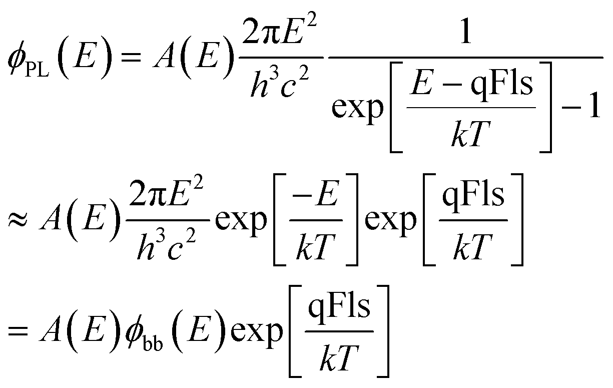 | (1) |
For a Shockley–Queisser approach, the absorptance spectrum is replaced by a step function at the band gap, which allows the determination of the Shockley–Queisser qFls (completely analogous to the Shockley–Queisser VOC):
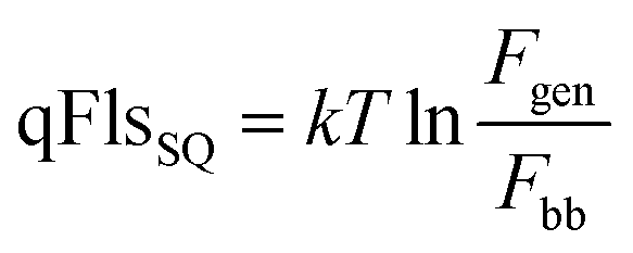 | (2) |
 | (3) |
The absolute measurement of ϕPL(E) allows the determination of the external radiative efficiency
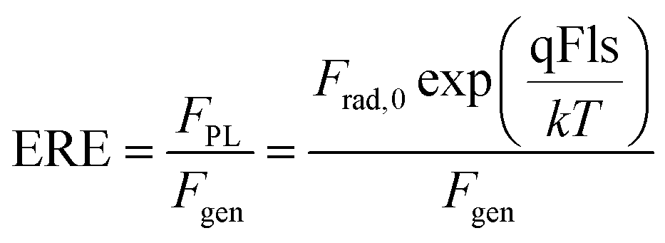 | (4) |
Reorganizing eqn (4) allows the determination of the qFls loss ΔqFlsnonrad resulting from non-radiative loss processes according to6,18,19
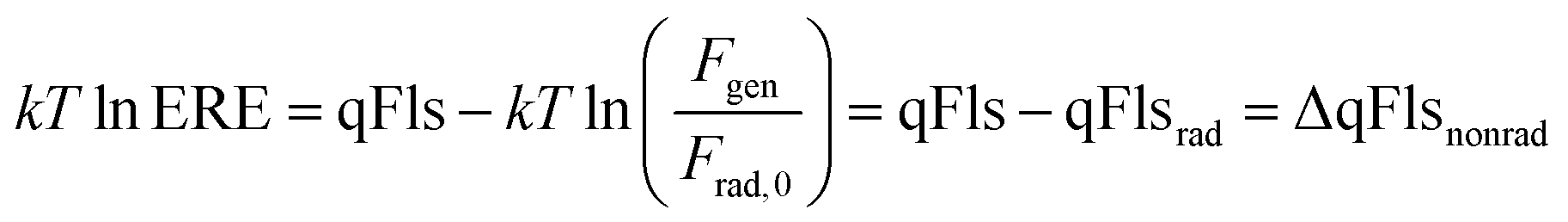 | (5) |
Thus, we are able to interpret the ERE as a relative loss term, i.e. a difference between the actual qFls and the qFlsrad that would be possible if only radiative recombination would take place in the material that has the actual absorptance A(E). The use of the ERE has been proven to be a powerful tool for the quantitative comparison of different photovoltaic materials and devices.12,15
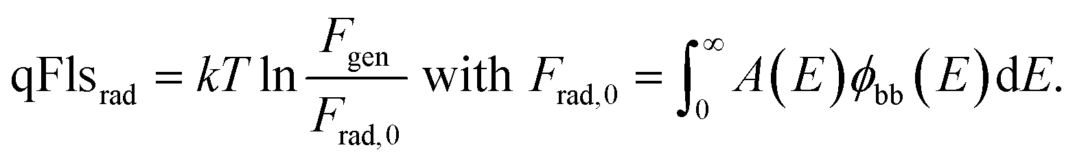
However, the determination of absolute values for qFls and qFlsrad requires measuring the absolute PL and, additionally, information or assumptions on the absorptance. Absolute PL has been described in many previous publications.3,4,20–22 Errors can occur in measuring the size of the laser spot and the laser power at the sample position, as well as in measuring the spectral power of the luminescence. These errors can be estimated by repeated calibrations and measurements and are in the range of a few meV. However, to simplify the analysis of the PL measurements, usually various assumptions are made. These simplifications introduce systematic errors that reduce the extracted qFls value compared to the real value, in general not by much, but a few 10 meV might play an important role when comparing different absorbers.
There are two fundamental ways to extract qFls from the calibrated PL measurements.4 The first one is based on eqn (5) and requires the knowledge of qFlsrad. The second one is based on a fit of the high energy slope of the PL peak to generalised Planck’s law, assuming that the absorptance is = 1 in this energy range. The problems and assumptions become obvious already. We discuss them in detail, together with ways to deal with them, for both methods.
Systematic errors in qFls from ERE
The method based on ERE and eqn (5) makes very few assumptions but requires the knowledge of qFlsrad. A proxy could be to use the qFlsSQ determined from the band gap. But determining the band gap of thin film materials can be difficult,23 in particular for emerging materials, which are not yet fully developed and can suffer from low quality. Various disorder effects can lead to tail states, which make it difficult to even define the band gap energy.24 Ideally, the band gap is determined from a measurement of the absorption coefficient, either by transmission–reflection measurements or by ellipsometry. Ellipsometry is often difficult in polycrystalline films because the surface roughness introduces significant uncertainty into the analysis. Although methods exist to correct for surface roughness in ellipsometry25,26 they are not designed to deal with a roughness of 100 nm or more, as is often observed in polycrystalline films. Therefore, it is very rare that optical data of polycrystalline films is determined by ellipsometry. Transmittance measurements, on the other hand, require transparent samples. Thin films for solar cells are often grown on a metallic back contact, rendering transmission measurements impossible. Either the films are removed mechanically from the back contact or films are grown in the same process onto a transparent substrate. The band gap determination is further hampered by band gap gradients along the depth of the sample, which are often intentional to reduce interface recombination.27–31 Similar to tail states, these gradients broaden the absorption onset. If the absorptance spectrum is known, the radiative qFlsrad can be determined, using eqn (3). In general, gradual onsets of the absorptance or the EQE spectrum make it difficult to determine the band gap.Recently, it has been proposed to use the derivative of the EQE onset to determine the PV band gap.16 A similar analysis is possible, using the absorptance spectrum instead of the EQE spectrum, as in eqn (2)–(5) above. Below, we discuss the possibility of extracting the absorptance spectrum from the PL spectrum. In general, for the reasons discussed above, separate absorptance measurements are not readily available, and usually the maximum of the PL emission is used as a proxy for the band gap, the “radiative” band gap.4,23 The argument for this approach is that radiative recombination is the only recombination in the ideal solar cell, so we should use the energy of the radiative recombination as the starting point for the detailed balance considerations. Using the energy of the PL maximum takes the radiative qFls loss already into account. However, in the case of a gradual slope at the absorption edge, this assumption is a simplification that leads to errors in the range of a few tens of meV, as shown below. The absorptance onset is gradual in materials that show a high density of tail states, that have a band gap gradient along the depth of the absorber or that are indirect semiconductors.16Table 1 compares the radiative loss and the shift of the luminescence spectrum for some of the solar cells in ref. 16 with respect to the PV gap EPVG, as defined in ref. 16. It can be seen that for those solar cells, where the luminescence is shifted with respect to the effective band gap (c-Si and CIGS), the actual radiative loss is in fact smaller by 15 to 20 mV than the implied radiative loss from the shift in the emission spectrum. Thus, using the PL maximum to determine qFlsrad in eqn (5) would underestimate the actual qFls by 15 to 20 meV.
| ΔVradOC | E PVG − Emaxluminescence | ΔVOC from shift | |
|---|---|---|---|
| c-Si | 66 | 90 | 84 |
| CIGS | 36 | 55 | 51 |
| CdTe | 30 | −2 | −1.5 |
| MAPIC | 6 | 0 | 0 |
This error is systematic, as becomes obvious from simulations using a Gaussian distribution P(EG) of the band gaps.32 It has already been shown in ref. 32 that with increasing the standard deviation σ of the distribution of band gaps, the emission peak shifts towards lower energies. An example is shown in the inset in Fig. 1. The maximum of the band gap distribution is at 1.2 eV and the emission maximum is shifted down to 1.16 eV with a width of σ = 40 meV, see the spectrum ϕG. By setting this energy as the band gap energy to subtract the non-radiative loss from, we assume that the effective Shockley–Queisser emission is given by the spectrum ϕpSQ (pseudo-Shockley–Queisser). Because the emission spectrum is based on the black body spectrum (eqn (1)), this emission would be stronger than the actual emission at a Shockley–Queisser type band gap of 1.2 eV (ϕSQ), implying a shorter radiative lifetime and lower qFls. The simulation allows the comparison of the two different losses of qFls. The green curve in Fig. 1 depicts the shift of the radiative qFlsrad due to the broadening of the band gap distribution from eqn (3). If using the PL maximum as the “radiative” band gap was correct, this loss would agree with the red curve, which represents the shift in the qFls due to the shift of the PL maximum, when assuming a Shockley–Queisser like band gap at the energy of the PL maximum. For small standard deviations, this loss is actually positive, i.e. the qFls is slightly larger than with a sharp band gap because the PL emission maximum increases in energy, mostly due to the E2 term in the generalised Planck’s law (see eqn (1)). But as the standard deviation approaches kT, the PL maximum shifts downwards and with it the corresponding pseudo-Shockley–Queisser qFls. With an increasing width of the band gap distribution, the PL maximum shifts more and more to lower energies,32 increasing the qFls loss. Beyond a width of 34 meV, the loss due to the shift of the “radiative” band gap becomes larger than the actual radiative loss. The difference quickly becomes larger than 10 mV. This difference is the error when replacing the radiative qFlsrad by the Shockley–Queisser qFls of a band gap of the PL maximum. When we then use qFlsSQ (with the PL maximum as the band gap) as a proxy for qFlsrad in eqn (5) to determine qFls, we make exactly this error in the range of 10 to 40 meV for realistic widths of the band gap distribution.
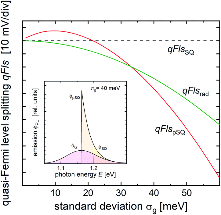 | ||
| Fig. 1 Different quasi Fermi level splittings qFls calculated for a model assuming a Gaussian distribution of band gap energies as a function of the standard deviation σg. The reference value qFlsSQ (dashed line) accounts for a step function like absorptance edge at the average band gap energy Eg,avg of the distribution, qFlsrad (green solid line) is the exact radiative value according to eqn (3), and qFlspSQ is the approximation to qFlsrad by assuming that the emission is Shockley–Queisser-type but at a band gap shifted to the maximum of the observed emission. Inset: simulated PL spectrum for a band gap distribution with σg = 40 meV (ϕG), together with the simulated Shockley–Queisser type emission spectrum for a band gap at the PL maximum (ϕpSQ) and at the real band gap (ϕSQ). | ||
Another source of error is the temperature in eqn (3) and (5). Very often, 25 meV is used for kT. But this is only 290 K, and usually the laboratory will be warmer. Another standard is assuming 25 °C or 300 K, corresponding to 25.7 meV and 25.8 meV, respectively. With a low radiative efficiency, the error in the obtained qFls is also on the order of 10 meV. It is therefore important to record and use the actual measurement temperature.
Systematic errors in qFls from fitting to generalised Planck’s law
The method based on the fitting to generalised Planck’s law does not require any assumptions about the band gap value, but introduces other errors. The main assumption is that the absorptance for energies in the high energy slope is A = 1.20–22 Then, according to eqn (1), qFls can determined from a linear fit to the log of the PL spectrum | (6) |
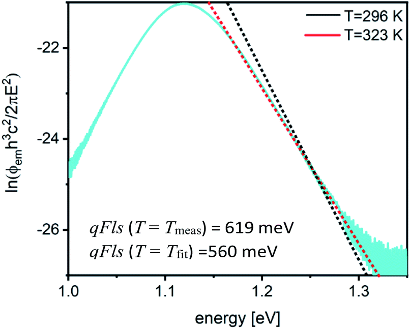 | ||
| Fig. 2 Replotted PL flux to extract qFls from the fit to generalised Planck’s law. The red line shows the fit with the temperature as a fit parameter, the black line shows the fit where the temperature has been fixed to the measurement temperature (296 K). The sample is a Cu(In,Ga)Se2 film. | ||
Using the correct temperature can balance the fact that the absorptance is not constant in the fitting range. The fact that A = 1 is not yet reached in this energy region, i.e. A < 1, is not balanced by this procedure. The smaller absorptance reduces the extracted qFls by −kTlnA. It is very unlikely that the absorptance in solar cell absorbers is very small at energies more than 100 meV above the band gap. If the absorptance was as low as 70% in the fitting range, the extracted qFls would underestimate the real one by about 10 meV, but in general the absorptance in the fitting range will be higher and the error smaller.
It is possible to extract a non-absolute absorptance spectrum from the PL spectrum: solving eqn (1) for the absorptance yields
 | (7) |
Thus, from the measured PL spectra, we are able to deduce the shape of the absorptance curve directly, albeit the qFls remains an unknown proportionality constant. Resolving eqn (1) for the qFls yields
 | (8) |
Note that the right hand side of eqn (8) contains the spectral quantities ϕPL(E), A(E) and ϕbb(E), whereas the left hand side is a fixed quantity. Thus, eqn (8) allows the checking of the consistency of the evaluation as the result should be the same for each photon energy E. Likewise, it is demonstrated that we need at least one reliable value for the absorptance A. One should further note that A stands for the absorptance of the PL active material, i.e. the material that is subject to the same qFls. Thus, any parasitic absorptance, e.g. provided by passivation layers or contacts, is not and must not be included. However, the absorptance of the absorber film itself can be influenced by the reflectivity of the back contact.
If the assumed qFls was too low, the extracted absorptance spectrum will be larger than the real one and can even take on unphysical values larger than 1. The best way to determine an exact qFls from the fit to generalised Planck’s law is to determine the absorptance spectrum separately. This can be done by ellipsometry, if the film is not too rough, or by photospectrometry, if the absorber film is grown on a transparent substrate or if it is possible to mechanically remove the film from a non-transparent substrate.
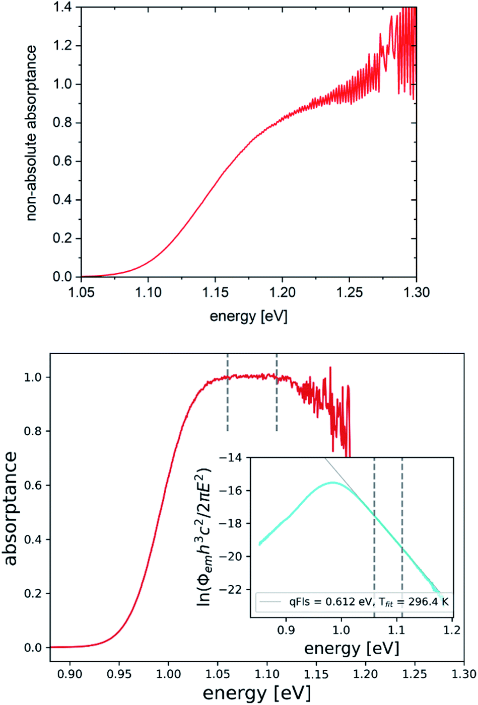
An example for a measurements on a methylammonium Sn iodide film is given in Fig. 3. The apparent temperature from the fit is 380 K (red fit line in Fig. 3 bottom). This is more than 100 K higher than the measurement temperature, which will lead to a greatly underestimated qFls. Unlike in Fig. 2, here it is not possible to force a fit with the correct measurement temperature. The qFls extracted from ERE and using the PL maximum for the “radiative” band gap is 870 meV. Using this qFls as a starting point, we can extract the non-absolute absorptance according to eqn (7). This extracted absorptance (Fig. 3, top) is strongly increasing within the fitting range and is above 1, which is unphysical. This sample was grown on glass and the true absorptance spectrum could be measured separately by photospectrometry. This film was rather thin and therefore the absorptance is far from reaching 1 within the possible fitting ranges for the PL spectrum. We can use the measured absorptance spectrum to correct the PL spectrum for a fit to Planck’s generalised law (light blue data Fig. 3, bottom, only the range with reliable A data is shown)
 | (9) |
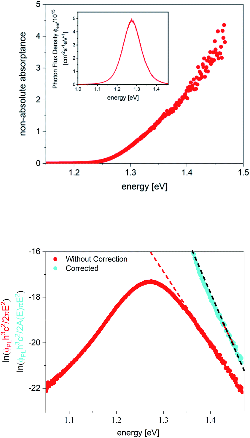 | ||
| Fig. 3 (Top) Non-absolute absorptance extracted from the PL spectrum in the inset. (Bottom) Replotted PL spectra for the fit to generalised Planck’s law, original (red) and divided by the separately measured absorptance spectrum (light blue). The fitting range is in both cases from 1.42 eV to 1.47 eV. The sample is a methylammonium Sn iodide film. | ||
The extracted qFls is now 940 meV (black fit line in Fig. 3, bottom). The fitted temperature is 290 K, only slightly lower than the measurement temperature. It should be noted that the fitted temperature depends on the fitting range and is even lower when using fitting ranges at lower energies. Thus, the high fitted temperature using eqn (6) is due to the fact that the absorptance spectrum is not flat in the fitting region, which can be corrected by eqn (9) using the separately measured absorptance spectrum. These considerations also show that the qFls determined from ERE is by 70 meV too low in this case.
Comparison of experimental results
The discussion in the last paragraph points out two major obstacles in obtaining the exact qFls of a solar cell absorber from PL measurements: the determination from ERE results is a systematic underestimation of the qFls, whereas the determination from the fit to generalised Planck’s law may not be possible or is also underestimated if the absorptance is not equal to 1 within the high energy slope of the PL peak.Fig. 4 shows the comparison between the qFls determined from ERE and those determined from the fit to Planck’s law, as well as the comparison with the VOC of the solar cells made from these absorbers. The comparison is made for various chalcopyrite solar cells, measured recently in our lab.
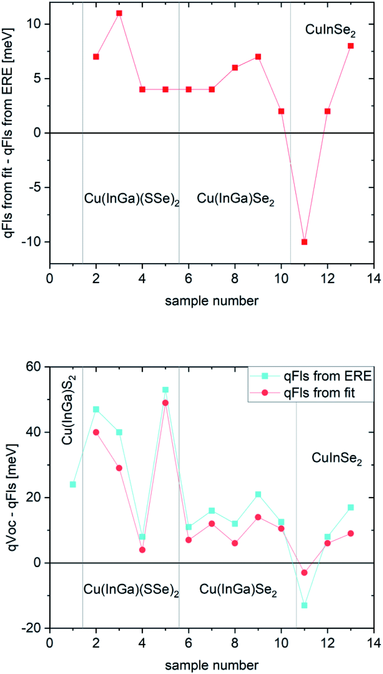 | ||
| Fig. 4 Comparison for various chalcopyrite solar cells. (Top) difference between qFls determined by the two different methods. (Bottom) Comparison between VOC and qFls. | ||
The first thing to notice is that, aside from sample #11, the qFls from ERE are lower than those from the fit. #11 is the highest quality sample: it shows the lowest FWHM of the PL spectrum, a fit temperature identical within error to the measurement temperature and a very high ERE of 1.5%. This sample is a CuInSe2 absorber with a Ga back gradient; the preparation and structure is explained in detail in ref. 35. All other samples have EREs below 10−3, some as low as 3 × 10⁻⁶ (sample 1 is not included in this plot since in this case the qFls determination from the fit is not possible; the fitted temperature is 463 K). This difference in the extracted qFls corroborates the systematic error of the ERE method to extract qFls. To understand the negative difference for sample #11, we can look at Fig. 1 (bottom): a slight broadening of the band gap distribution leads to an overestimation of qFls by the ERE method. The width of the PL spectrum can be taken as an indication of the width of the distribution. Sample #11 has the smallest FWHM of all samples considered here. This could indicate that it also has the smallest width of the band gap distribution, which could be in the range where the ERE method overestimates qFls, thereby explaining why the qFls from the fit to generalised Planck’s law is lower. The other samples show a tendency to have a larger mismatch between the two determined qFls values when the FWHM is larger (see Fig. 5). We would like to point out that there is nothing wrong with determining the non-radiative loss from ERE. Eqn (5) is correct. But using the energy of the PL maximum as a proxy for the band gap introduces an underestimation of the qFlsrad. Based on the discussion above, it appears that the fit to generalised Planck’s law is the more reliable way to determine qFls, when it is possible. The second graph in Fig. 5 compares VOC with qFls. Only the very good sample #11 behaves as expected: the VOC is lower than the detected qFls. #11 is also the only sample where the fitted temperature is less than 5 K different from the actual measurement temperature. This observation indicates that qFls from the fit is also underestimated if the assumption of A = 1 is not met, as discussed above. When we only consider the comparison with the “better” qFls value obtained from the fit (Fig. 4 bottom), the discrepancy between qVOC and qFls is lower than 15 meV, besides the three Cu(In,Ga)(S,Se)2 samples, which show metastable effects and will be discussed later. The discrepancy between the fitted temperature and the measurement temperature can be used as an indication of how much the real situation is removed from the assumption of A = 1. The difference between VOC and qFls shows a tendency to increase with this temperature difference (Fig. 5).
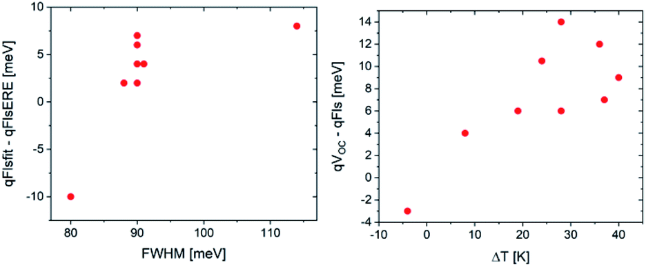 | ||
| Fig. 5 Trends of the errors: discrepancy between the two methods to determine qFls as a function of the FWHM of the PL peak and the discrepancy between VOC and qFls from the fit to generalised Planck’s law as a function of the discrepancy between the fitted temperature and the measurement temperature. | ||
It is possible to directly check if the assumption of A = 1 holds using eqn (7). The non-absolute absorptance spectrum extracted from the PL spectrum of Fig. 2 is shown in Fig. 6 (top). Although the absorption edge is clearly visible and the absorptance begins to level off after the step, it continues to increase and increases beyond A = 1. This is a Cu(In,Ga)Se2 sample with an intentional Ga double gradient, which explains why the absorptance does not level off right after the absorption edge, which is determined by the minimum band gap in the notch of the gradient.36 Unfortunately, the PL spectrum becomes very noisy at high energies. If it was possible to reliably measure PL towards higher energies, it might be possible to observe the levelling off of the absorptance spectrum. The qFls determined using the assumption A = 1 is smaller than the real qFls, thus the absorptance spectrum will level off at a value >1, as indicated in Fig. 6 (top). The apparent value of A(E → ∞) is given by exp(qFlsreal/kT)/exp(qFlsmeas/kT), where qFlsreal is the real qFls and qFlsmeas is the measured qFls, allowing the rescaling of the absorptance spectrum and determination of a more reliable qFls. A more reliable absorptance spectrum is shown in Fig. 6 (bottom). It shows the PL spectrum of sample #11 in the inset, together with a new fit with the temperature as fit parameter. It results in the same value as the measurement temperature. The extracted absorptance in this case levels off beyond the absorption edge and reaches a value of 1, without any further adjustments. We believe that the apparent decrease of the absorptance at higher energies is an artefact due to the noise in the PL spectrum. Both the levelling off of the A spectrum and the correct fit temperature indicate that in this case, the qFls is reliable. In this case, the assumption A = 1 in the fit range is correct, making the extracted absorptance spectrum an absolute one. Sample #11 has the lowest FWHM of the PL, which is due to a steeper absorption edge, and the highest ERE, which allows a reliable determination of the absorptance at high enough energies, where A levels off. For this sample, in fact, the VOC is lower than the qFls, as expected.
 | ||
| Fig. 6 Non-absolute absorptance spectra extracted from PL spectra using eqn (7). Top: from PL spectrum in Fig. 2, bottom: from sample #11 (replotted PL spectrum shown in the inset). Vertical lines indicate the fit range. | ||
Other sources of error
For most samples discussed so far, the discrepancy between qFls and qVOC is smaller than 15 meV. But the three Cu(In,Ga)(S,Se)2 samples show much larger differences, between 30 and 50 meV. All Cu(In,Ga)(S,Se)2 samples show the distinct feature that both the VOC and qFls depend significantly on the wavelength of the excitation, as demonstrated in Fig. 7. In most cases, the qFls is higher when the sample is illuminated by the blue laser than when it is illuminated by the red laser. This is not a phenomenon that we generally observe in other samples. With the exception of sample 2 under red illumination, the VOC is lower than qFls under the same illumination, as expected. And for most samples, VOC is considerably larger under simulated AM1.5 illumination than under red or blue illumination. It is important to note that in all cases, the illumination was controlled to ensure that the number of photons is identical to the number of photons above the band gap in an AM1.5 spectrum. Thus, the large discrepancy between the qFls and VOC is due to the dependence of VOC (and qFls) on the wavelength of the excitation. The cause of this behaviour is not understood yet. It is likely that metastable defects play a role here.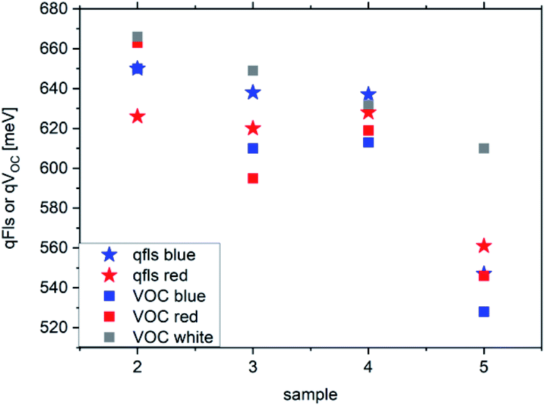 | ||
| Fig. 7 qFls and VOC for the Cu(In,Ga)(S,Se)2 samples illuminated with a red laser (660 nm), a blue laser (405 nm) or a simulated AM1.5 spectrum (white). | ||
Another effect that we observed in some samples is an upward shift in the PL spectrum by about 10 meV after finishing the solar cell. This behaviour is also not understood yet, but certainly contributes to the discrepancy between qFls and VOC.
Distribution of SQ-band gaps
In an analogy to a recent description of the electroluminescence16 of solar cells, we use here an arbitrary distribution P(Eg) of Shockley–Queisser type band gap energies to describe the PL emission by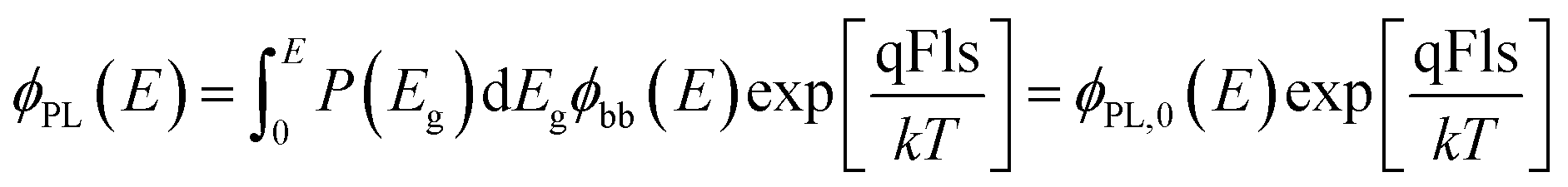 | (10) |
With the above assumptions, the absorptance is given by the integral over step-function-like contributions (as in the SQ-model) weighted by the distribution P(Eg) according to
 | (11) |
Eqn (11) allows us to determine the distribution P(Eg) from the derivative
 | (12) |
Note that from eqn (11), we have
 | (13) |
Fig. 8a shows the measured PL emission (red solid line) that is used to calculate a non-scaled absorptance A with the help of eqn (7). In a second step, a non-scaled probability distribution P(Eg) is determined using eqn (12). For the scaling of P(Eg), we use the assumption that the integral  (from Eg = 1 eV to 1.23 eV) equals 0.8 (see Fig. 8b). This assumption, in turn, implies that we fix the absorptance at a value A(1.23 eV) = 0.8, as shown in Fig. 8c, where the red line depicts the scaled data from the measurement and the symbols the reconstructed data, which unsurprisingly fit the original data because they just result from the differentiation and reintegration of the original data. From the scaled absorptance spectrum, we are able to calculate the saturation spectrum ϕPL,0(E) [eqn (10)], shown by the blue curve in Fig. 8a. Note that the factor exp(qFls/kT) that is used to shift the spectrum ϕPL,0(E) to the originally measured one in Fig. 8a is the same that is used to scale the band gap distribution P(Eg) in Fig. 8b and to scale the absorptance spectrum A(E) in Fig. 8c. With a generation current density Fgen = 2.7 × 1017 cm−2, we arrive at a qFls = 623 mV and at qFlsrad = 890 mV. The ERE = 2.8 × 10⁻⁵ is then obtained by eqn (4).
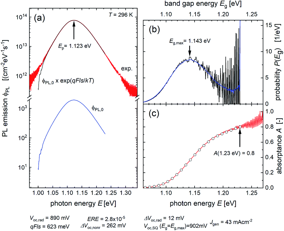 | ||
Fig. 8 (a) Measured PL emission ϕPL (red line) and reconstructed saturation emission ϕPL,0 (blue). The thin black line corresponds to ϕPL,0 × exp(qFls/kT) and fits the original data. (b) Distribution P(Eg) of band gap energies normalized to 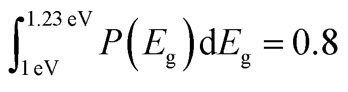 (black: original data, blue: smoothed). (c) Extracted (red line) and reconstructed (symbols) absorptance A. Both spectra are normalized to A(1.23 eV) = 0.8. (black: original data, blue: smoothed). (c) Extracted (red line) and reconstructed (symbols) absorptance A. Both spectra are normalized to A(1.23 eV) = 0.8. | ||
Obviously, the critical step during this procedure is the need for fixing the scale of the band gap distribution P(Eg). As can be seen in Fig. 8b, the high energy end of P(Eg) is poorly defined due to the noise in the original data, the high energy end of the PL spectrum with very low intensity. Therefore, the distribution method faces the same difficulties as the other two methods when aiming for the determination of the absolute values for the qFls and the radiative qFlsrad, namely the lack of knowledge of absolute values of the absorptance A. Thus, we have to live with regard to this restriction with an uncertainty of up to 10 meV in the determined qFls. However, the method provides us with some additional information, like the width and the maximum (1.143 eV, Fig. 8c) of the band gap distribution.
Conclusions
We have discussed the different methods to determine the qFls from absolute photoluminescence and their systematic errors that lead to an underestimation of the qFls. The main reason for the systematic errors is the fact that the absorptance spectrum is generally not known.When using the PL maximum as the “radiative” band gap energy to determine the qFls from ERE, using eqn (5), the qFls is underestimated because the PL shift in general overestimates the radiative loss. This error increases the broader the PL peak is. Using a fit to Planck’s generalised law gives only an exact value for qFls if the absorptance in the fitting range is constant and = 1. If this assumption is not met, the fitted temperature will be larger than the measurement temperature. The larger the discrepancy in the temperature, the more underestimated the qFls will be. Yet, if the fitted temperature is less than 30 K different from the measurement temperature, the qFls determined from the fit with the temperature fixed to the measurement temperature is more reliable than the one determined from ERE.
It should be pointed out that for well-behaved PL spectra, the errors discussed here are typically smaller than 20 meV.
For not too broad PL spectra, reliable, but non-absolute absorptance spectra can be extracted. Based on these, a separate analysis of the distribution of band gaps is possible, in an analogy to the detailed balance analysis of EQE.16
When the goal is to compare the quality of different samples, it is more reliable to directly compare the ERE values,15 in combination with the width of the PL spectra. The better samples have higher ERE and a narrower PL peak. When the goal is to predict the VOC or to compare with actual VOC values, the fit to generalised Planck’s law should be used. If the fit temperature is higher than the measurement temperature, a separately measured absorptance spectrum is needed to the fit to obtain the exact qFls. If the discrepancy in the temperature is smaller than 30 K, a fit with the temperature fixed to the measurement temperature is possible.
In spite of the errors discussed in this paper, PL is an extremely useful tool to determine the quality of absorbers for solar cells, before finishing the solar cells.
Author contributions
SuS initiated and supervised the study and wrote the first version of the manuscript. UR provided the model for and initiated and provided the simulations. SG, TPW, TW, DA, AS prepared the samples analysed. SG, TPW, AP, TW, DA, MD performed the PL measurements and the various data analyses. Everybody contributed to the discussion and revision of the manuscript.Conflicts of interest
There are no conflicts to declare.Note added after first publication
This article replaces the version published on 5th August 2022, which contained an error in eqn (1).Acknowledgements
Financial support from the Luxembourgish Fonds National de la Recherche (FNR) in the framework of the projects TAILS, PACE, MASSENA and SUNSPOT is gratefully acknowledged. The company Avancis, Germany, is thankfully acknowledged for providing the Cu(In,Ga)(S,Se)2 samples. We thank Prof. Alex Redinger and his team at the University of Luxembourg for providing the Sn perovskite sample. Prof. Ayodhya Tiwari and his team at EMPA, Switzerland provided sample #11, which is gratefullyacknowledged.Notes and references
- T. Kirchartz and U. Rau, Adv. Energy Mater., 2018, 8, 1703385 CrossRef.
- R. Scheer and H. W. Schock, Chalcogenide Photovoltaics: Physics, Technologies, and Thin Film Devices, Wiley-VCH, 2011 Search PubMed.
- T. Kirchartz, J. A. Márquez, M. Stolterfoht and T. Unold, Adv. Energy Mater., 2020, 10, 1904134 CrossRef CAS.
- S. Siebentritt, T. P. Weiss, M. Sood, M. H. Wolter, A. Lomuscio and O. Ramirez, J. Phys.: Mater., 2021, 4, 042010 CAS.
- A. Lomuscio, T. Rödel, T. Schwarz, M. Melchiorre, D. Raabe and S. Siebentritt, Phys. Rev. Appl., 2019, 11, 054052 CrossRef CAS.
- W. Shockley and H. J. Queisser, J. Appl. Phys., 1961, 32, 510–519 CrossRef CAS.
- P. Würfel, Physics of Solar Cells, Wiley-VCH, Weinheim, 2005 Search PubMed.
- W. van Roosbroeck and W. Shockley, Phys. Rev., 1954, 94, 1558–1560 CrossRef CAS.
- J. I. Pankove, Optical Processes in Semiconductors, Dover Publications, New York, 1975 Search PubMed.
- U. Rau, V. Huhn and B. E. Pieters, Phys. Rev. Appl., 2020, 14, 014046 CrossRef CAS.
- M. Sood, A. Urbaniak, C. K. Boumenou, H. Elanzeery, F. Babbe, F. Werner, M. Melchiorre, A. Redinger and S. Siebentritt, Progr. Photovolt.: Res. Appl., 2022, 30, 263, DOI:10.1002/pip.3483.
- M. A. Green, Prog. Photovolt.: Res. Appl., 2012, 20, 472–476 CrossRef CAS.
- T. P. Weiss, F. Ehre, V. Serrano-Escalante, T. Wang and S. Siebentritt, Sol. RRL, 2021, 5, 2100063 CrossRef CAS.
- T. Trupke, R. A. Bardos, M. D. Abbott and J. E. Cotter, Appl. Phys. Lett., 2005, 87, 093503 CrossRef.
- L. Krückemeier, U. Rau, M. Stolterfoht and T. Kirchartz, Adv. Energy Mater., 2020, 10, 1902573 CrossRef.
- U. Rau, B. Blank, T. C. M. Müller and T. Kirchartz, Phys. Rev. Appl., 2017, 7, 044016 CrossRef.
- P. Würfel, J. Phys. C: Solid State Phys., 1982, 15, 3967–3985 CrossRef.
- U. Rau, Phys. Rev. B: Condens. Matter Mater. Phys., 2007, 76, 085303 CrossRef.
- R. T. Ross, J. Chem. Phys., 1967, 46, 4590–4593 CrossRef CAS.
- L. Gütay, R. Pomraenke, C. Lienau and G. H. Bauer, Phys. Status Solidi A, 2009, 206, 1005–1009 CrossRef.
- T. Unold and L. Gütay, in Advanced Characterization Techniques for Thin Film Solar Cells, ed. D. Abou-Ras, T. Kirchartz and U. Rau, Wiley, 2011, pp. 151–176 Search PubMed.
- F. Babbe, L. Choubrac and S. Siebentritt, Appl. Phys. Lett., 2016, 109, 082105 CrossRef.
- S. Siebentritt, G. Rey, A. Finger, J. Sendler, T. P. Weiss, D. Regesch and T. Bertram, Sol. Energy Mater. Sol. Cells, 2016, 158, 126–129 CrossRef CAS.
- G. Rey, G. Larramona, S. Bourdais, C. Choné, B. Delatouche, A. Jacob, G. Dennler and S. Siebentritt, Sol. Energy Mater. Sol. Cells, 2018, 179, 142–151 CrossRef CAS.
- G. Badano, P. Ballet, J.-P. Zanatta, X. Baudry, A. Million and J. W. Garland, J. Opt. Soc. Am. B, 2006, 23, 2089–2096 CrossRef CAS.
- D. Lehmann, F. Seidel and D. R. T. Zahn, SpringerPlus, 2014, 3, 82 CrossRef PubMed.
- A. M. Gabor, J. R. Tuttle, M. H. Bode, A. Franz, A. L. Tennant, M. A. Contreras, R. Noufi, D. G. Jensen and A. M. Hermann, Sol. Energy Mater. Sol. Cells, 1996, 41–42, 247–260 CrossRef.
- T. Feurer, B. Bissig, T. P. Weiss, R. Carron, E. Avancini, J. Löckinger, S. Buecheler and A. N. Tiwari, Sci. Technol. Adv. Mater., 2018, 19, 263–270 CrossRef CAS PubMed.
- T. P. Weiss, B. Bissig, T. Feurer, R. Carron, S. Buecheler and A. N. Tiwari, Sci. Rep., 2019, 9, 5385 CrossRef PubMed.
- T. Wang, T. P. Weiss, F. Ehre, B. Veith-Wolf, J. Schmidt, V. Titova, N. Valle, M. Melchiorre and S. Siebentritt, Adv. Energy Mater., 2021 Search PubMed.
- X. Zheng, D. Kuciauskas, J. Moseley, E. Colegrove, D. S. Albin, H. Moutinho, J. N. Duenow, T. Ablekim, S. P. Harvey, A. Ferguson and W. K. Metzger, APL Mater., 2019, 7, 071112 CrossRef.
- U. Rau and J. Werner, Appl. Phys. Lett., 2004, 84, 3735 CrossRef CAS.
- R. Carron, E. Avancini, T. Feurer, B. Bissig, P. A. Losio, R. Figi, C. Schreiner, M. Burki, E. Bourgeois, Z. Remes, M. Nesladek, S. Buecheler and A. N. Tiwari, Sci. Technol. Adv. Mater., 2018, 19, 396–410 CrossRef CAS PubMed.
- G. Rey, C. Spindler, S. Siebentritt, M. Nuys, R. Carius, S. Li and C. Platzer-Björkman, Phys. Rev. Appl., 2018, 9, 064008 CrossRef CAS.
- T. Feurer, R. Carron, G. T. Sevilla, F. Fu, S. Pisoni, Y. E. Romanyuk, S. Buecheler and A. N. Tiwari, Adv. Energy Mater., 2019, 9, 1901428 CrossRef.
- M. H. Wolter, B. Bissig, E. Avancini, R. Carron, S. Buecheler, P. Jackson and S. Siebentritt, IEEE J. Photovoltaics, 2018, 8, 1320–1325 Search PubMed.
Footnote |
| † In the ideal solar cell, current is not limited by a finite mobility and thus will proceed without a Fermi level gradient. |
| This journal is © The Royal Society of Chemistry 2022 |