 Open Access Article
 This Open Access Article is licensed under a
 Creative Commons Attribution 3.0 Unported Licence
Electron-induced dissociation dynamics studied using covariance-map imaging†
David
Heathcote
 *,
Patrick A.
Robertson
,
Alexander A.
Butler
,
Cian
Ridley
,
James
Lomas
,
Madeline M.
Buffett
,
Megan
Bell
and
Claire
Vallance
*
*,
Patrick A.
Robertson
,
Alexander A.
Butler
,
Cian
Ridley
,
James
Lomas
,
Madeline M.
Buffett
,
Megan
Bell
and
Claire
Vallance
*
Department of Chemistry, University of Oxford, Chemistry Research Laboratory, 12 Mansfield Road, Oxford, OX1 3TA, UK. E-mail: david.heathcote@chem.ox.ac.uk; claire.vallance@chem.ox.ac.uk
First published on 18th April 2022
Abstract
Recently, covariance analysis has found significant use in the field of chemical reaction dynamics. When coupled with data from product time-of-flight mass spectrometry and/or multi-mass velocity-map imaging, it allows us to uncover correlations between two or more ions formed from the same parent molecule. While the approach has parallels with coincidence measurements, covariance analysis allows experiments to be performed at much higher count rates than traditional coincidence methods. We report results from electron-molecule crossed-beam experiments, in which covariance analysis is used to elucidate the dissociation dynamics of multiply-charged ions formed by electron ionisation over the energy range from 50 to 300 eV. The approach is able to isolate signal contributions from multiply charged ions even against a very large ‘background’ of signal arising from dissociation of singly-charged parent ions. Covariance between the product time-of-flight spectra identifies pairs of fragments arising from the same parent ions, while covariances between the velocity-map images (‘recoil-frame covariances’) reveal the relative velocity distributions of the ion pairs. We show that recoil-frame covariance analysis can be used to distinguish between multiple plausible dissociation mechanisms, including multi-step processes, and that the approach becomes particularly powerful when investigating the fragmentation dynamics of larger molecules with a higher number of possible fragmentation pathways.
1 Introduction
Unimolecular reactions involve an evolution of the reactant A into products P, i.e. reaction follows the equation A → P, and include processes such as dissociation and isomerisation. As shown though Lindemann’s pioneering insight,1 unimolecular reactions in general do not occur in a single step, but instead involve an (often bimolecular) excitation step followed by the unimolecular reaction of interest, i.e.| A + M ⇌ A* + M | (1) |
| A* → P | (2) |
The Lindemann mechanism above involves collisional activation of the reactant A by another atom or molecule M, which in practice is often another A molecule. However, excitation can occur via a number of methods, including collisional excitation, photoexcitation and electron ionisation.2–5 The present manuscript focuses on processes in which excitation occurs via electron ionisation.
Significant work has been undertaken during the past century to further our understanding of unimolecular reactions. One of the fundamental theories describing statistical unimolecular reactions is the Rice–Ramsperger–Kassel (RRK) theory,6,7 which was later developed into Rice–Ramsperger–Kassel–Marcus (RRKM) theory,8 in parallel with the development of quasiequilibrium theory.9,10 RRKM theory has found many uses; for example, it has been used to predict molecular breakdown diagrams for a variety of molecules;5,9,11–16 if the rate of formation of each set of products is known as a function of energy, then the branching ratio for each fragment can be found as a function of energy. This enables prediction of experimental observables such as mass spectra. Mass spectra have also been predicted using both non-dynamical quantum methods17–22 and dynamical quantum methods, typically utilising Born–Oppenheimer molecular dynamics (BOMD) and related techniques.23,24
Statistical models such as RRKM theory rely on the molecule having sufficient time for the internal energy to equilibrate amongst the energetically accessible states prior to dissociation. The models can also be used to predict the unimolecular decay of molecular ions; following ionisation there is often a rapid cascade of radiationless transitions due to numerous curve crossings between electronic states, which usually results in the formation of ions with a broad “statistical” distribution of internal energies, almost irrespective of the lifetime of the ion.12 Even if the ion is initially formed with a high degree of electronic excitation, this rapid relaxation cascade has the result that dissociation generally occurs from one of a few low-lying electronic states. Sometimes, rapid dissociation from a strongly repulsive state competes with energy redistribution to the extent that the resulting product velocity and internal energy distributions are distinctly non-statistical.25,26
In our previous work studying the electron-induced dissociation dynamics of singly-charged ions, we have observed both statistical and non-statistical dissociation processes. For example, in our work on the unimolecular dissociation of CF3I+,27 we found that the most likely fragmentation pathways, involving the breaking of either a C–F or the C–I bond, display markedly different dynamics following cleavage of the two types of bond. Following C–F bond cleavage, the charge resides exclusively on the CF2I+ ion. CF2I+ is formed with a kinetic energy distribution peaking away from zero, implying an impulsive dissociation mechanism. In contrast, C–I bond cleavage yields both CF3+ and I+ products. These are formed with a kinetic energy distribution peaking at or close to zero, consistent with a slower “statistical” dissociation process. The kinetic energy distribution for I+ in fact peaked slightly away from zero, implying the presence of a weakly repulsive exit channel for formation of I+, while the kinetic energy distribution of the CF3+ products could be fitted well by the statistical ‘model free’ approach developed by Klots.28 Comparison of the measured fragment kinetic energy distributions with data from photoelectron ionisation experiments, in which individual electronic states are accessed, enabled us to assign the most likely electronic states from which dissociation occurs in each case.
We have drawn a number of conclusions on the process of dissociative electron ionisation from our previous work. The kinetic energies of the detected ions are very small relative to the energy of the incident electron, implying that the majority of the available energy is carried away by the two departing electrons. This is perhaps unsurprising given that the timescale of the ionisation process (10−17 to 10−16 s) is much too fast for significant energy to be coupled into nuclear motion. In addition, the kinetic energy distributions for fragments formed from singly charged parent ions show essentially no dependence on incident electron energy. This is a result of the rapid relaxation processes alluded to above: the product ion kinetic energy distributions are determined by the topography of the potential energy surface corresponding to the dissociating electronic state, not the initially accessed state. Similar dynamics have been observed for the products of singly-charged ion dissociation in almost all of the non-diatomic molecules we have studied to date.27,29,30 The remainder of the manuscript will therefore focus on the unimolecular dissociation of multiply-charged parent ions.
As the charge on the ion increases, the dynamics become dominated by Coulomb repulsion between the charges. Dissociation generally becomes increasingly rapid, with Coulomb explosions occurring on the timescale of a few tens of femtoseconds.31–34 However, despite the Coulomb repulsion, even multiply-charged ions can sometimes exist in metastable states that survive for significant periods of time. The existence of such ions is often revealed in time-of-flight (ToF) measurements by long “tails” on the corresponding ion ToF peaks, caused by the ions dissociating as they traverse the field-free flight tube after clearing the extraction region of the mass spectrometer.35–37
A number of techniques have been used to study the unimolecular decay of multiply-charged ions, including tandem mass spectrometry,38–42 photoelectron–photoion–photoion coincidence (PEPIPICO)43–47 and covariance-map imaging.31,36,48–51 Covariance analysis of multimass velocity-map imaging datasets is a powerful technique which allows correlations between ions formed from the same individual molecule or cluster to be observed. First introduced by Frasinski et al. as a method to allow correlations to be uncovered under experimental conditions where coincidence experiments are unattainable,31 it has since found widespread use under such conditions, for example in experiments carried out at free electron laser facilities.50,52–55
In this work, we highlight the use of covariance mapping to determine the dissociation mechanisms of multiply-charged ions for a selection of molecules formed via electron ionisation. Using a combination of ToF–ToF covariance and recoil-frame covariance, insight into the unimolecular dissociation of multiply-charged ions can be obtained.
2 Experimental
The electron-molecule crossed beam experiment has been discussed in detail previously,27,56 but will be briefly summarised here.A pulsed molecular beam was generated via expansion of the sample gas through a pulsed solenoid valve (Hannifin-Parker Series 9 general valve), operating at a frequency of 25 Hz. In this work, we consider three molecules of interest: trifluoroiodomethane (CF3I), sulfur dioxide (SO2), and furan. CF3I and SO2 are gases at room temperature and, with the exception of the CF3I experiments performed at an electron energy of 100 eV for which a neat beam of CF3I was used, the samples were prepared by forming a gas mix with helium at 12.5% for CF3I and approximately 15% for SO2. The backing pressure was typically set to approximately 3.5 bar. Furan is a liquid at room temperature, and was prepared by bubbling helium at a pressure of 1.5 bar through the liquid.
The molecular beam was crossed with a pulsed electron beam from one of two sources. At electron energies of 100 eV and below, a PSP Vacuum Technology ELS 100 electron gun was used, with pulsing achieved by applying a negative potential 40 V in excess of the electron energy to the final electronic lens element within the gun, which was switched to ground to allow electron pulses to enter the interaction region. At electron energies in excess of 100 eV, an Ionoptika IOE10 electron source was used, pulsed by applying a switching potential of −400 V to the “blanking” lens within the source’s electrostatic lens assembly. The molecular and electron beams intersect between the grounded extractor and repeller electrodes of a velocity-map imaging (VMI) ion lens.57
After the electron beam has cleared the interaction region, the extractor and repeller electrodes were rapidly switched to their operating potentials using a pair of fast transistor switches (Behlke model HTS-101). Any ions generated were accelerated along the flight tube towards a position-sensitive detector consisting of a pair of chevron-mounted microchannel plates (MCPs), coupled to a P47 phosphor. Each ion arriving at the MCPs generates a spot of light on the phosphor, which is recorded using a Pixel Imaging Mass Spectrometry (PImMS) sensor. For every detected ion, the x, y and t coordinate is recorded. The arrival time t is proportional to the mass-to-charge ratio of the ion, while the (x, y) coordinates are proportional to its x, y velocity components in the centre of mass frame. The (x, y, t) data set can be integrated over the x and y coordinates to obtain a mass spectrum. Alternatively, the data can be integrated over a range of t corresponding to the arrival time of a given ion of interest to obtain the corresponding scattering distribution. The ion optics used in our experiments cause all ions of the same m/z to arrive at the detector at the same time, so the recorded scattering distributions are two-dimensional projections of the full three-dimensional distributions. The three-dimensional scattering distributions can be obtained from the 2D images using an inverse Abel transform method such as BASEX.58 The scattering distribution is usually considered in terms of the angular and kinetic energy distributions for each ion of interest.
2.1 Covariance analysis
Provided that two or more ions are formed and detected from the same parent molecule, we can use covariance analysis to reveal the correlations between either the arrival times of the ions, known as ToF–ToF covariance, or to show correlations between their velocity vectors, known as recoil-frame covariance.Covariance analysis in the context of velocity-map imaging experiments has been discussed in detail in recent reviews.50,51,59 Mathematically, covariance is a simple statistical measure of correlation between two variables, obtained using the following equation
| cov(X,Y) = 〈(X − 〈X〉)(Y − 〈Y〉)〉 = 〈XY〉 − 〈X〉〈Y〉 | (3) |
We have previously found that we need to account for variation in experimental parameters over time, such as the molecular beam density and electron current. To rationalise the need to account for such variation, consider the case in which one of these parameters varies. The overall signal will clearly increase or decrease as a function of the varying parameter. Since all ion signals increase or decrease as a function of the varying parameter, a positive covariance is observed between all ions, and this experimental artefact can mask the ‘true’ covariance arising from the dissociation dynamics. Covariance arising from experimental drift can be corrected by utilising either partial or contingent covariance.50,59–63 For all covariance maps presented here, we use partial covariance, given by the following equation
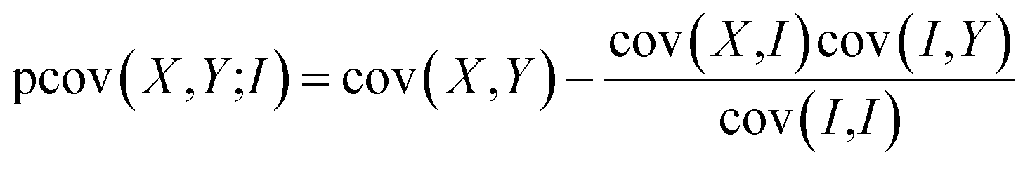 | (4) |
![[thin space (1/6-em)]](https://www.rsc.org/images/entities/char_2009.gif) 000 s or greater.
000 s or greater.
As noted above, ToF–ToF covariance maps reveal the correlation between the arrival times of the various fragment ions, and are plotted as a 2D array where each pixel represents the covariance between two arrival times, ti and tj. A diagonal self-covariance feature is observed, i.e. where i = j, which corresponds to the variance of the ToF spectrum. Any off-diagonal features then show correlations between the formation of two ions from the same parent ion. The gradients of these features are related to the relative momenta of the two ions along the time-of-flight axis of the experiment.43,51,64 This grants us an insight into the mechanism of the associated unimolecular decay. For example, for the two-body dissociation of ABC2+ to form A+ + BC+, the two ion fragments would have equal and opposite momenta, and thus a feature with a gradient of minus one would be observed. For the case of a three-body decay, the dissociation can occur via any of the following mechanisms:
| ABC2+ → A+ + B+ + C | (5) |
| ABC2+ → A+ + BC+ → A+ + B+ + C | (6) |
| ABC2+ → AB2+ + C → A+ + B+ + C | (7) |
Mechanism (5) is a concerted dissociation, where the molecule dissociates in a single step. The gradient of the ToF–ToF covariance map in this case depends on the nature of the dissociation process, but it can often be assumed that the neutral C fragment carries only a small proportion of the momentum, in which case ions A and B will have approximately equal and opposite momenta, resulting in a gradient very close to −1.51 Mechanism (6) is an “initial charge separation” process, in which the two charges separate in an initial step, followed by the loss of a neutral fragment. The gradient can be found to be 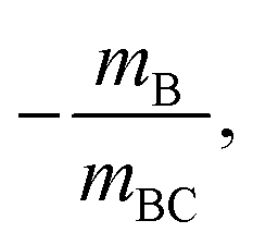 assuming there is sufficient time between the two steps for the molecular orientation prior to the second dissociation to be unrelated to that of the first.43,64 Mechanism (7) is a “deferred charge separation” process, in which a neutral is lost first, followed by the charge separation step. The gradient for this process can be found to be −1, again assuming the two dissociation steps can be treated independently.43,64
We also see false covariance signals in our data, which typically appears as cross features with positive covariance on the positive gradient, and negative covariance on the negative gradient. False covariance signals can arise due to the presence of a varying parameter, as discussed above, or due to statistical noise not perfectly cancelling out.
Recoil-frame covariance maps show the correlation between the velocity vectors of two ions. One of the ions is chosen as the ‘reference’ ion, and a second is chosen to be the ‘signal’ ion. For each acquisition cycle, the velocity vectors of both signal and reference ions are rotated such that the reference ion velocities lie along a selected reference direction, indicated by an arrow in the corresponding figures. The resulting covariance map shows the velocity distribution of the signal ion relative to the reference ion. For a more complete description of the recoil-frame covariance technique, see our recent review in ref. 51.
3 Results and discussion
3.1 Furan
To demonstrate the power and versatility of covariance analysis, we have chosen three chemical systems with varying degrees of chemical complexity, from which we can gain clear mechanistic insight. Firstly, we examine the dissociation of furan2+, following double electron ionisation of neutral furan at 100 eV. Furan is an unsaturated heterocyclic molecule that is often used as a model for the deoxyribose moiety of the DNA backbone. Single ionisation of furan has been shown to induce dissociation via two major pathways, in which C–O bond cleavage is accompanied by either C![[double bond, length as m-dash]](https://www.rsc.org/images/entities/char_e001.gif) C or C–C cleavage.65 Here, we will focus purely on the unimolecular dissociation of multiply-ionised furan.
C or C–C cleavage.65 Here, we will focus purely on the unimolecular dissociation of multiply-ionised furan.
From the various cross-peaks observable in the ToF–ToF covariance map shown in Fig. 1, it is apparent that there are a number of dissociation channels available to the furan dication. Here we will only focus on the primary two-body dissociation pathways. It is clear that there are two dominant fragmentations of the molecular backbone, resulting in the formation of either C3H3+ + CHO+ or C2H2+ + C2H2O+. Of the two pathways, there is a strong preference for the dissociation to form C3H3+ + CHO+.
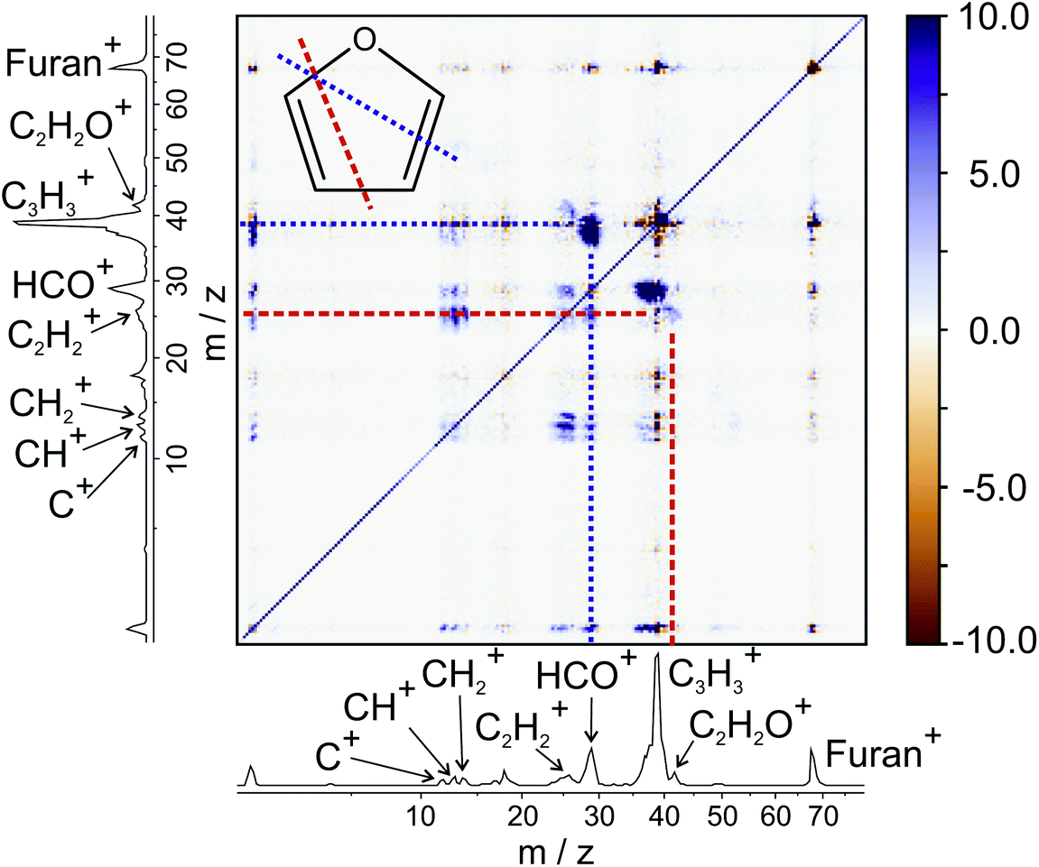 | ||
| Fig. 1 ToF–ToF covariance maps of furan obtained at 100 eV. The fragments referred to in the text have been labelled. Note that the diagonal is an axis of symmetry. The molecular structure of furan is inset, with the bonds which are required to break to form C3H3+ and HCO+, and C2H2+ and C2H2O+ indicated by a purple dotted line and an orange dashed line, respectively. The corresponding features are highlighted on the ToF–ToF covariance map. | ||
Fig. 2 shows the recoil-frame covariance maps obtained for these two two-body dissociation pathways, along with the momentum distributions of the ions. The reference ion is constrained to lie along the reference direction indicated and, due to conservation of linear momentum, the velocity vector of the corresponding signal ion lies in the opposite direction. As with the scattering distributions typically obtained from a velocity-map imaging experiment, the radius of the image is proportional to the velocity of the ion. The ‘tail’ extending to the centre of the image is an artefact arising from the fact that we carry out covariance analysis between velocity-map images, which are 2D projections of the full scattering distribution. We are currently developing an inversion procedure which will allow us to correct for this, as well as exploring the use of 3D covariance-map imaging,66 which avoids the problem entirely. From the kinetic energy distributions, we are able to obtain a kinetic energy release of approximately 5.0 eV for the C3H3+/CHO+ channel, and of approximately 5.5 eV for the C2H2+/C2H2O+ channel. Kinetic energy releases for these processes do not appear to have been reported previously.
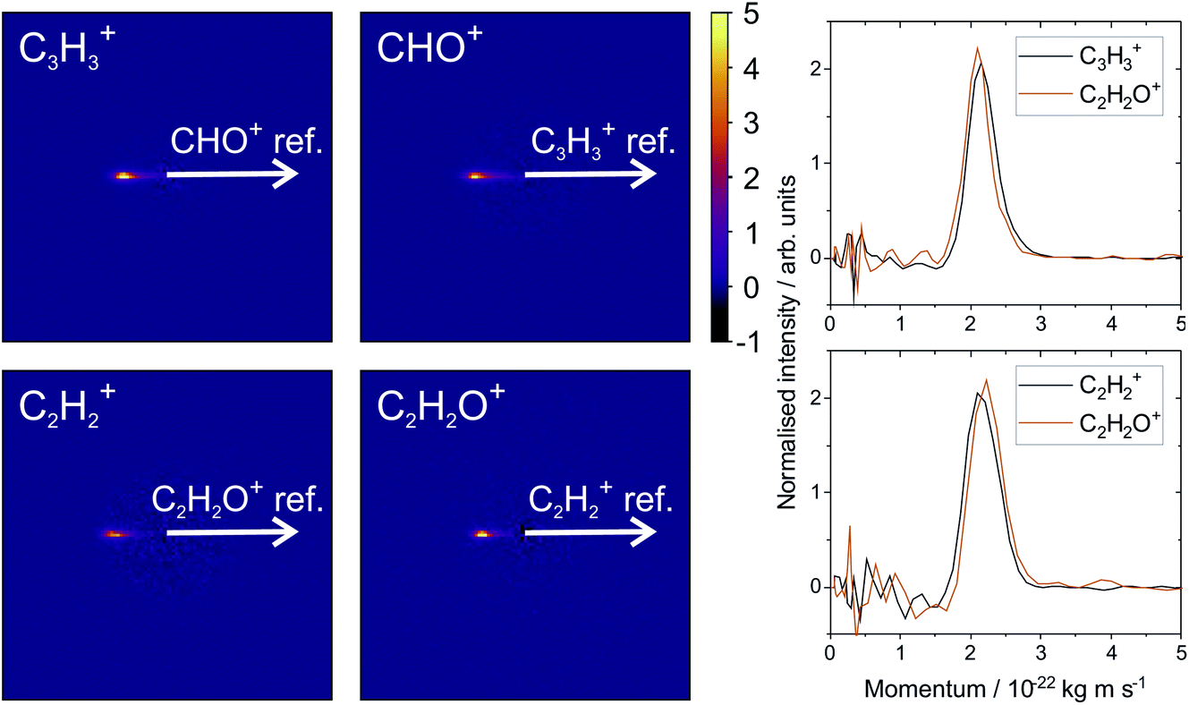 | ||
| Fig. 2 Recoil-frame covariance images obtained following electron ionisation of furan at an electron energy of 100 eV, between C3H3+ and HCO+, and C2H2+ and C2H2O+. All covariance maps show the characteristic form of a two-body dissociation. The corresponding momentum distributions given on the right show that momentum is conserved as expected. | ||
3.2 Trifluoroiodomethane
In our second example, we report the dissociation dynamics of CF3I2+ formed by electron ionisation of CF3I at electron energies in the range 100 eV to 300 eV. The data recorded at 100 eV has been published previously,27,56, but the data recorded at 200 eV and 300 eV is previously unpublished. Singly-charged CF3I is widely used as a model compound for dissociative dynamics experiments.56,67–70 Here, we show how recoil-frame covariance analysis allows us to disentangle mechanistic information from a vast array of competing dissociation channels for higher charge states of CF3I.Following our work on the dissociation of the CF3I+ monocation discussed previously, we recently studied the unimolecular dissociation of multiply-charged CF3I ions in the energy range 100 to 300 eV. Using covariance analysis, we can isolate the signal arising from these ions, while excluding the much larger signal contribution from the dissociation of CF3I+. The doubly and triply-charged parent ions typically fragment to form a CFn+ ion, an I+ ion, and 3 − n neutral fluorine atoms. If we consider the three-body decay involving loss of a single neutral fluorine atom then, as discussed earlier, there are three possible dissociation mechanisms for the CF3I2+ dication
| Concerted: CF3I2+ → CF2+ + I+ + F | (8) |
| Initial-charge separation: CF3I2+ → CF3+ + I+ → CF2+ + I+ + F | (9) |
| Deferred-charge separation: CF3I2+ → CF2I2+ + F → CF2+ + I+ + F | (10) |
For the two-step processes (9) and (10) we were able to perform Monte-Carlo simulations to predict the relative velocity distributions obtained through covariance analysis of the two ionic fragments, assuming the two dissociation steps can be treated independently of one another. We found that at an electron energy of 100 eV the dissociation was best described by a combination of both initial and deferred charge separation processes, with a greater weighting for dissociation via the deferred charge separation mechanism. This was consistent with the work of Douglas,71 who found that at 50 eV, initial charge separation was the dominant dissociation mechanism, whilst at 200 eV the situation is reversed. We have recently repeated the measurements at both 200 eV and 300 eV (see Fig. 3 and S1†), and in contrast to the findings of Douglas, while we do perhaps observe a slight increase in the relative contribution of deferred charge separation, we do not see a drastic change in the relative velocity distributions, and therefore the dissociation mechanism, at these higher energies. Further investigation is warranted in order to determine the source of this discrepancy.
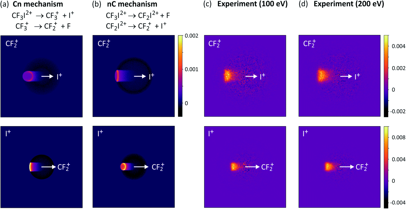 | ||
| Fig. 3 Simulated covariance-map images for the unimolecular dissociation of CF3I2+ for an (a) initial charge separation (mechanism (10), labelled Cn) and a (b) deferred charge separation (mechanism (10), labelled nC) process, compared with (c) and (d) experimentally measured covariance maps recorded at electron energies of 100 eV and 200 eV, respectively. For the top row of covariance maps, I+ is the reference ion and CF2+ is the signal ion, and vice versa for the bottom row. (a)–(c) are reprinted with permission from ref. 56. Copyright 2020 Taylor & Francis Ltd. | ||
For the dissociation channels observed at lower electron energies, we do not see any significant changes in the dissociation dynamics as the electron energy is increased. However, we do see new dissociation channels opening up at higher energies. Fig. 4 shows the mass spectrum of CF3I obtained at 100 eV, 200 eV, and 300 eV. In addition to the fragment ions we previously reported, we also observe CF2I2+, CI+, CF+, and CFI+ at 100 eV. By 200 eV, we see the appearance of a small number of new ions, namely C2+, F2+, and I3+, though with insufficient signal intensity to plot the corresponding scattering distributions.
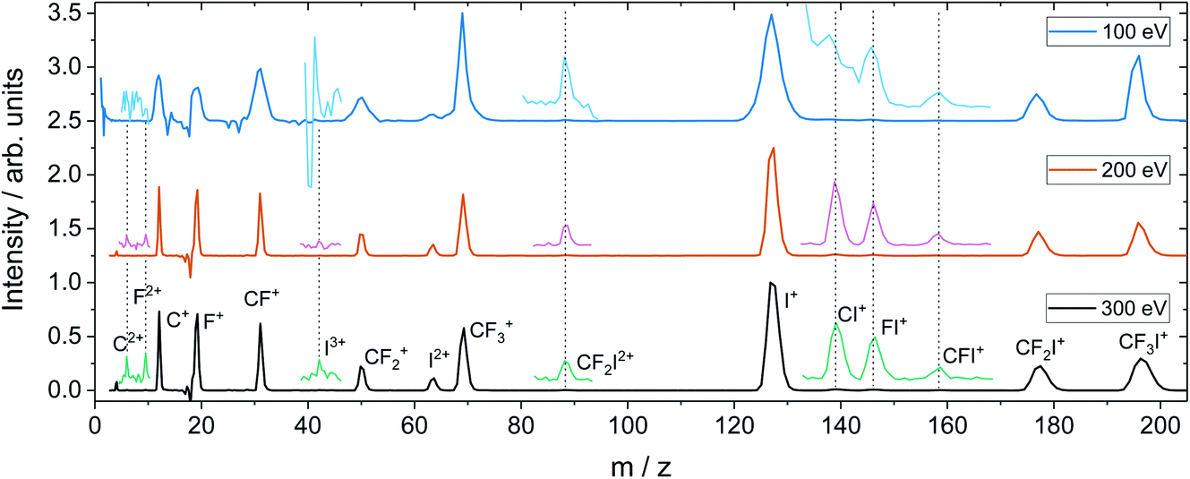 | ||
| Fig. 4 Time-of-flight spectrum recorded for CF3I at 100, 200, and 300 eV, with baselines of 2.50, 1.25 and 0.00, respectively. The spectra have been normalised such that the I+ peak has a maximum intensity of one. Less intense peaks are shown magnified by a factor of 50, and offset from the baseline by 0.1. Note that for the 100 eV data, the CI+ and CF+ peaks fall on the shoulder of the I+ peak. | ||
Fig. 5 shows the partial ToF–ToF covariance maps obtained for CF3I at the same three electron energies. In the following we will use the notation “(X+,Y+)” to denote a covariance between X+ and Y+ fragment ions, referring to this as the “(X+,Y+) covariance channel”. At an electron energy of 100 eV, we observed covariance between the following ion pairs: (I+/2+,CF3+), (I+/2+,CF2+), (I+/2+,CF+), (I+/2+,C+), (I+,F+), (C+,F+) and (CF+,F+). At an electron energy of 200 eV, we observe the additional covariances (CI+,F+) and (F+,F+), and the (much weaker) covariances (C+,F2+), (C+,FI+) (I+,C2+), (I+,F2+), (I2+,C2+), (F+,C2+) and (F+,F2+). By 300 eV we also observe weak covariance between the ion pairs (F2+,I2+) and (C+,I3+). ToF–ToF spectra plotted on a more saturated colour scale to highlight these weaker covariance signals can be found in the ESI.†
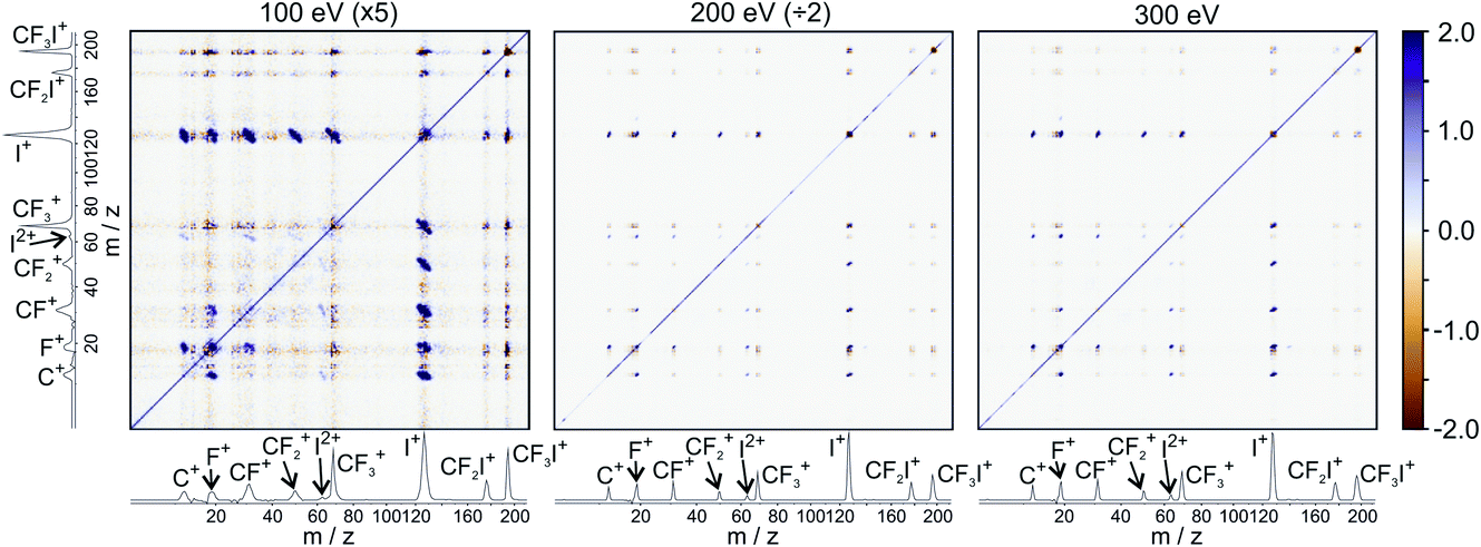 | ||
| Fig. 5 ToF–ToF covariance maps obtained following electron ionisation of CF3I at electron energies of 100, 200, and 300 eV. Saturated ToF–ToF covariance maps for the 200 and 300 eV data, in which weaker covariance signals are visible, can be found in the ESI.† | ||
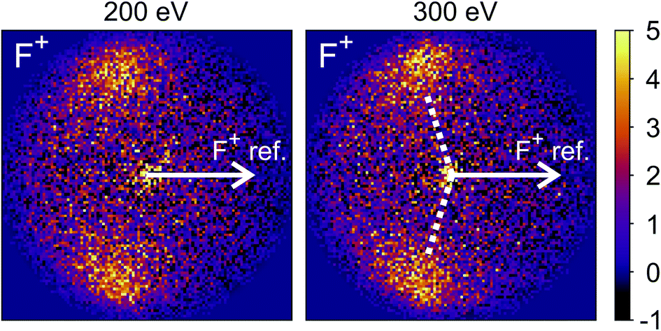
The new channels appearing at higher electron energies, which we predominantly attribute to the dissociation of the CF3I trication, almost all have insufficient signal to allow for a recoil-frame covariance map to be generated, but for some channels we can construct these maps and gain further insight into the dissociation mechanism. Fig. 6 shows the covariance map for the (F+,F+) channel at 200 and 300 eV. It is clear that the two F+ ions are generated in a concerted manner, as there is very little intensity opposite to the reference direction, and the covariance signal appears in a well-defined location. In a multi-step process, the relative velocities would typically be blurred to a greater extent, due to scrambling of the fragment orientations between steps. Given the energetically unfavourable nature of forming two F+ ions, presumably a third charged fragment is also being generated. Covariance maps showing the correlation of F+ with all other partner fragments at 300 eV are shown in Fig. 7. Of these co-fragments, I+ and I2+ show by far the strongest covariance with F+, and the angle between the F+ and the I+ in the covariance image is entirely consistent with a rapid dissociation dominated by Coulomb repulsion. It is worth noting that the covariance signal in the I2+ covariance map appears more well-resolved. This is perhaps a result of the shorter lifetime of the tetracation relative to the trication, allowing less opportunity for structural rearrangements to occur prior to dissociation, which might ‘blur’ the observed recoil-frame covariance. The covariance signal for the other three co-fragments is significantly less well defined. However, both the (CF+,F+) and (C+,F+) covariance maps have a similar form to that seen for the covariance maps involving I+. The similarity between the angular distributions for these two covariance channels implies that they follow a very similar mechanism. The weak covariance signal for the (CI+,F+) channel has a well-defined relative velocity vector, but also a much smaller velocity component perpendicular to the F+ reference direction than for any of the other fragment pairs discussed here. This leads us to the conclusion that this channel comes about predominantly as a result of the dissociation of CF3I2+ as, if the trication was formed, a third F+ ion must be generated. The repulsion between the two F+ ions would lead to a significant velocity component perpendicular to the direction of travel of the CI+ fragment similar to that observed in the (I+,F+) channel, which we do not observe.
 | ||
| Fig. 6 Recoil-frame covariance images obtained at 200 and 300 eV between F+ and F+. The well-defined covariance implies a rapid, concerted dissociation on a repulsive potential energy surface. The white dotted lines indicate the angle at which covariance signal is obtained when modelling the dissociation of CF3I4+ to form I2+ and two F+ using a simple Coulomb model, as discussed in the text. | ||
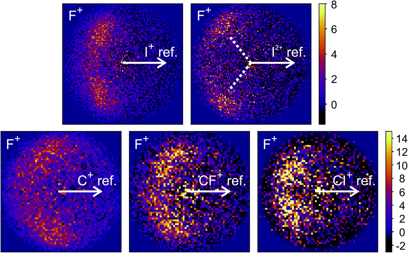 | ||
| Fig. 7 Recoil-frame covariance images obtained at 300 eV between F+ and I+, I2+, C+, CF+, and CI+. Note that where C+, CF+ and CI+ are reference ions, the corresponding covariance maps have been rebinned to a greater extent to improve the signal-to-noise ratio. Corresponding covariance images where the F+ ion has been used as the reference ion can be found in the ESI.† In the (I2+,F+) covariance map, the white dotted lines indicate the angle at which covariance signal is obtained when modelling the dissociation of CF3I4+ to form I2+ and two F+ using a simple Coulomb model, as discussed in the text. | ||
We have also carried out simulations using a simple Coulomb model for the dissociation of CF3I4+ to form I2+, 2F+, and neutral fragments. Details of the simulations can be found in the ESI,† but the recoil angles obtained through the simulations are indicated by dotted lines in the (F+,F+) and (I2+,F+) covariance maps shown in Fig. 6 and 7, respectively. We see that, even with a simple model, we are able to predict the recoil direction of the fragments with a good degree of accuracy, lending support to our proposed mechanism. We cannot rule out a contribution from dissociation of the trication, with the neutral fragment(s) being generated with significant kinetic energy, but this mechanism seems less likely.
Our results for CF3I+ at 200 and 300 eV reveal clear mechanistic and structural insight into the dissociation of highly-charged cations against the “background” of other ions formed from the ensemble of parent cation states formed in the initial electron ionisation process. Further analysis using three-fold covariance methods61,62 will enable us to confirm or refine these tentative mechanistic assignments.
3.3 Sulfur dioxide
For our final example, we will consider the electron ionisation of the simple triatomic SO2 over the electron energy range from 50 to 100 eV. The total and partial electron ionisation cross sections for SO2 have been reported previously.72–74 At 200 eV, double and triple ionisation account for 31% and 3% of the total ion yield, respectively.75 At lower electron energies the proportion of double ionisation to triple ionisation increases, with the result that triple ionisation only makes a relatively small contribution to our signal. Our discussion will thus focus on the dissociation of the SO2 dication.Fig. 8 shows the ToF–ToF covariance maps obtained for SO2 following electron ionisation at 50, 75, and 100 eV. In the following, we will focus purely on the (S+,O+) covariance channel, with other channels to be discussed in a future publication. As noted previously, the gradient of the ToF–ToF covariance map grants an insight into the dissociation mechanism. The gradient of the (S+,O+) covariance peak is seen to be approximately −1 at all electron energies, consistent with either a concerted or deferred charge separation process. In our experiments we are unable to distinguish between these two mechanisms using ToF–ToF covariance alone. However, by studying the recoil-frame covariance maps, we are granted a greater insight into the dissociation mechanism.
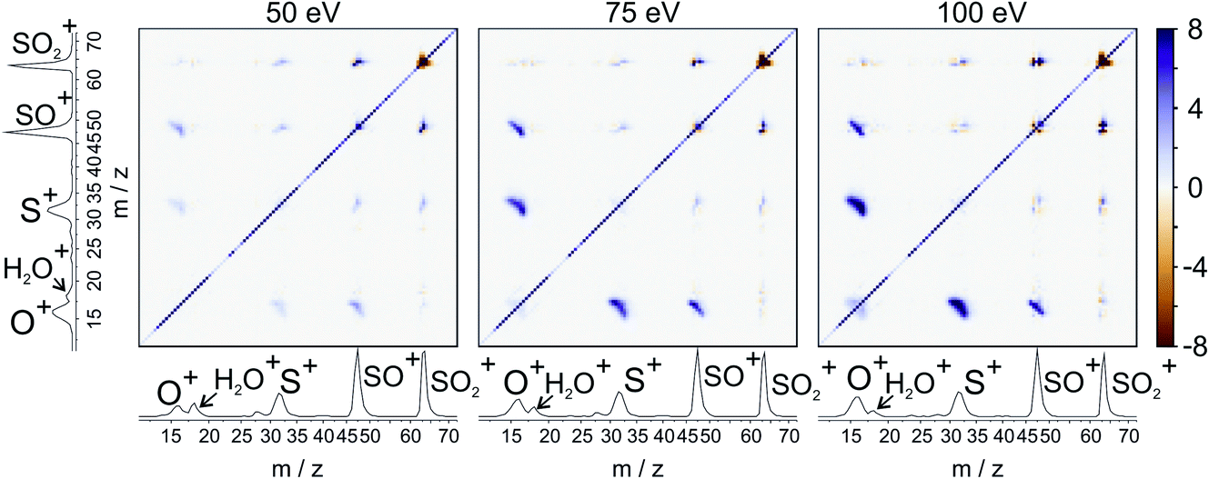 | ||
| Fig. 8 ToF–ToF covariance maps for the dissociative electron ionisation products of SO2 obtained at 50, 75, and 100 eV. The main features are covariances between O+ and both SO+ and S+. | ||
Fig. 9 shows the covariance images obtained for the formation of S+ and O+ following electron ionisation of SO2 at electron energies of 50, 75 and 100 eV. We see a clear change in the relative velocity distribution, and therefore presumably the dominant dissociation pathway, over the energy range 50 to 100 eV.
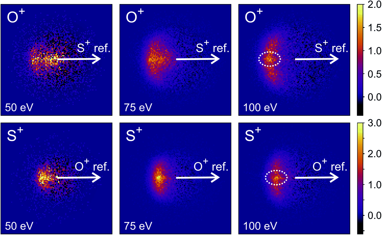 | ||
| Fig. 9 Recoil-frame covariance images obtained for dissociative ionisation of SO2 electron energies of 50, 75 and 100 eV for the (S+,O+) covariance channel. For the 100 eV covariance maps, a weak feature corresponding to the dissociation of SO23+ to form either S2+ and O2+ or S+ and O22+ has been highlighted. | ||
There has been significant discussion in the literature on this particular dissociation channel of SO22+.35,74–82 In photoionisation experiments, a clear change in the kinetic energy distributions of the fragments has been observed between photon energies of 40 and 60 eV.74 Fletcher et al. have reported the cross-sections for formation of each ion fragment following electron ionisation of SO2, and observe a rapid increase in the cross-section for formation of both S+ and O+ following electron ionisation between 50 and 100 eV.75 At 50 eV, the dissociation is best described as a deferred charge separation process, i.e. via the mechanism
| SO22+ → SO2+ + O → S+ + O+ + O | (11) |
SO2+ is observed as a weak signal in our data, so it seems probable that, provided the SO2+ has sufficient internal energy, it will dissociate. This mechanism has also been proposed previously by Eland and co-workers as a possible dissociation pathway for the formation of S+ and O+.35,79,81
As the electron energy is increased, the mechanism moves closer to a concerted pathway, i.e. dissociation occurs via the mechanism
| SO22+ → S+ + O+ + O | (12) |
Hsieh and Eland also proposed a process in which one of the S–O bonds lengthens prior to dissociation, but the neutral O atom is still weakly bound to the (short-lived) SO2+ dication at the point of dissociation.79 This mechanism is the most consistent with our findings at 100 eV; the arc feature seen in the O+ covariance map (top right, Fig. 9) shows that O+ is evolved with a well-defined velocity relative to S+, with a relatively uniform distribution over a range of angles. The S+ covariance map shows a vertical feature, which implies that S+ ions travelling in the opposite direction to the O+ ion have a marginally lower velocity than those with a velocity component perpendicular to the motion of O+. These observations are entirely consistent with the mechanisms discussed above. If the neutral O is still loosely bound to the sulfur atom of the SO2+ fragment when dissociation occurs, the O+ ion will be unimpeded, which results in the well-defined velocity for the fragment. However, the S+ will interact with the neutral O to varying degrees. It is known that ionic structures are often highly fluctional,12 and thus we expect the molecular ion to dissociate from a range of O–S–O bond angles. As shown in Fig. 10, where the SO2 molecule is far from linear, the S+ ion will undergo a glancing collision with the neutral O, which will change the direction of recoil of the S+ relative to the O+, but the magnitude of its velocity will be relatively unchanged. However, as the SO2 structure becomes more linear, the S+ will become impeded by the neutral O, and a greater proportion of its momentum from the Coulomb repulsion will be transferred to the O. This results in the S+ having a lower velocity, as we observe. Provided our mechanistic assignment is correct, the lifetime of the precursor SO2+ dication decreases with increasing electron energy, leading to the change in mechanism observed over the 50 to 100 eV electron energy range.
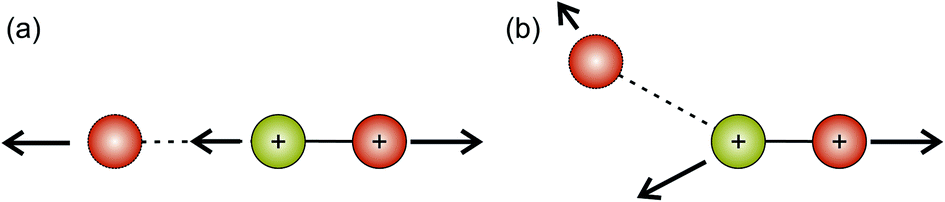 | ||
| Fig. 10 Proposed dissociation mechanism of SO2 at an electron energy of 100 eV for the (S+,O+) covariance channel. The red atoms correspond to oxygen, and the green-yellow atoms to sulfur. (a) Shows the case where the SO22+ dication is linear. In this case, the departing S+ ion is hindered by the presence of the neutral O atom, leading to a smaller kinetic energy than might otherwise have been the case. (b) Shows a case where the SO22+ dication is bent. The kinetic energy of the S+ ion is greater than in case (a), but the trajectory is deflected due to the presence of the neutral O. | ||
Careful inspection of the covariance maps in Fig. 9 also reveals a weak but well-defined signal in a direction directly opposite to the reference direction, highlighted in Fig. 9. This distribution is characteristic of a two-body dissociation, and in this case almost certainly results from the dissociation of SO23+ to form S2+ and O2+. These fragment ions have the same m/z ratios as O+ and S+ respectively, and will therefore contribute to the velocity-map images for these masses and hence the covariance-map images. Another possible explanation for the feature is the formation of S+ and O22+ from SO23+.
4 Conclusions
We have presented results demonstrating the use of covariance analysis to study unimolecular dissociation channels of multiply-charged furan, CF3I and SO2. We are able to use the results of our analysis to propose plausible dissociation mechanisms from a selection of possible outcomes. The ability to perform covariance analysis lies in the fact that there is a great deal of additional information within multi-mass imaging data sets which is not available when each ion is imaged separately. Covariance analysis allows us to pull out correlations between the identities and velocities of different ions, yielding insight into the dissociation mechanism. In our work to date, ToF–ToF covariance has revealed a variety of different fragmentation channels, with additional channels observed to open up at higher electron energies. Recoil-frame covariance-map images have revealed a number of different fragmentation mechanisms, with the dominant mechanism for production of a given ion pair often changing with the collision energy of the electron-molecule collision in which the parent ion is formed is increased. It is evident that covariance analysis is a powerful technique for studying the unimolecular decay of multiply charged ions.Author contributions
CV conceived the experiments and secured funding. DH and CR performed the experiments on furan. DH, PAR and MMB performed the experiments on CF3I. DH, PAR, AAB, JL and MB performed the experiments on SO2. DH analysed the data and prepared the figures. AAB carried out the Coulomb explosion simulations for CF3I with assistance from DH. DH, PAR, AAB and CV discussed the results in detail. DH prepared the manuscript with assistance from PAR. CV edited the manuscript.Conflicts of interest
There are no conflicts to declare.Acknowledgements
This work was supported by the EPSRC under Programme Grants EP/L005913/1 and EP/T021675/1, and a Doctoral Training grant to AAB. MMB acknowledges funding by a Hertford College Summer Research Studentship.References
- F. A. Lindemann, S. Arrhenius, I. Langmuir, N. R. Dhar, J. Perrin and W. C. McC. Lewis, Trans. Faraday Soc., 1922, 17, 598–606 RSC.
- M. L. Vestal, J. Chem. Phys., 1965, 43, 1356–1369 CrossRef.
- S. Gordon, G. Krige and N. Reid, Int. J. Mass Spectrom. Ion Phys., 1974, 14, 109–124 CrossRef CAS.
- K. Stephan, T. Märk and A. Castleman Jr, J. Chem. Phys., 1983, 78, 2953–2955 CrossRef CAS.
- M. Foltin, M. Lezius, P. Scheier and T. D. Märk, J. Chem. Phys., 1993, 98, 9624–9634 CrossRef CAS.
- O. K. Rice and H. C. Ramsperger, J. Am. Chem. Soc., 1927, 49, 1617–1629 CrossRef CAS.
- L. S. Kassel, J. Phys. Chem., 1928, 32, 225–242 CrossRef CAS.
- R. A. Marcus, J. Chem. Phys., 1952, 20, 359–364 CrossRef CAS.
- H. M. Rosenstock, M. B. Wallenstein, A. L. Wahrhaftig and H. Eyring, Proc. Natl. Acad. Sci. U. S. A., 1952, 38, 667–678 CrossRef CAS PubMed.
- C. E. Klots, Z. Naturforsch. A, 1972, 27, 553–561 CAS.
- C. Lifshitz, Acc. Chem. Res., 1994, 27, 138–144 CrossRef CAS.
- J. C. Lorquet, Int. J. Mass Spectrom., 2000, 200, 43–56 CrossRef CAS.
- L. Drahos and K. Vékey, J. Mass Spectrom., 2001, 36, 237–263 CrossRef CAS PubMed.
- E. E. Rennie, L. Cooper, C. A. Johnson, J. E. Parker, R. A. Mackie, L. G. Shpinkova, D. M. Holland, D. A. Shaw and M. A. Hayes, Chem. Phys., 2001, 263, 149–165 CrossRef CAS.
- E. A. Solano and P. M. Mayer, J. Chem. Phys., 2015, 143, 104305 CrossRef PubMed.
- B. West, S. Rodriguez Castillo, A. Sit, S. Mohamad, B. Lowe, C. Joblin, A. Bodi and P. M. Mayer, Phys. Chem. Chem. Phys., 2018, 20, 7195–7205 RSC.
- I. Mayer and Gömöry, Int. J. Quantum Chem., 1993, 48, 599–605 CrossRef.
- I. Mayer and Gömöry, J. Mol. Struct.: THEOCHEM, 1994, 311, 331–341 Search PubMed.
- R. Improta, G. Scalmani and V. Barone, Int. J. Mass Spectrom., 2000, 201, 321–336 CrossRef CAS.
- I. Mayer and Á. Gömöry, Chem. Phys. Lett., 2001, 344, 553–564 CrossRef CAS.
- P. A. Wright, A. Alex and F. Pullen, Rapid Commun. Mass Spectrom., 2014, 28, 1127–1143 CrossRef CAS PubMed.
- J. A. Schüler, S. Neumann, M. Müller-Hannemann and W. Brandt, J. Mass Spectrom., 2018, 53, 1104–1115 CrossRef PubMed.
- S. Grimme, Angew. Chem., Int. Ed., 2013, 52, 6306–6312 CrossRef CAS PubMed.
- C. A. Bauer and S. Grimme, J. Phys. Chem. A, 2016, 120, 3755–3766 CrossRef CAS PubMed.
- C. Galloy, C. Lecomte and J. C. Lorquet, J. Chem. Phys., 1982, 77, 4522–4528 CrossRef CAS.
- M. Roorda, A. J. Lorquet and J. C. Lorquet, J. Phys. Chem., 1991, 95, 9118–9121 CrossRef CAS.
- H. Köckert, D. Heathcote, J. W. Lee, W. Zhou, V. Richardson and C. Vallance, Phys. Chem. Chem. Phys., 2019, 21, 14296–14305 RSC.
- C. E. Klots, Z. Phys. D, 1991, 21, 335–342 CrossRef CAS.
- J. N. Bull, J. W. Lee and C. Vallance, Phys. Rev. A, 2017, 96, 42704 CrossRef.
- D. Heathcote, D. Phil. thesis, University of Oxford, 2020.
- L. J. Frasinski, K. Codling and P. A. Hatherly, Science, 1989, 246, 1029–1031 CrossRef CAS PubMed.
- F. Légaré, K. F. Lee, I. V. Litvinyuk, P. W. Dooley, A. D. Bandrauk, D. M. Villeneuve and P. B. Corkum, Phys. Rev. A, 2005, 72, 52717 CrossRef.
- C. S. Slater, S. Blake, M. Brouard, A. Lauer, C. Vallance, C. S. Bohun, L. Christensen, J. H. Nielsen, M. P. Johansson and H. Stapelfeldt, Phys. Rev. A, 2015, 91, 53424 CrossRef.
- W. Zhou, L. Ge, G. A. Cooper, S. W. Crane, M. H. Evans, M. N. Ashfold and C. Vallance, J. Chem. Phys., 2020, 153, 184201 CrossRef CAS PubMed.
- T. A. Field and J. H. Eland, Chem. Phys. Lett., 1993, 211, 436–442 CrossRef CAS.
- P. Wang and C. R. Vidal, Chem. Phys., 2002, 280, 309–329 CrossRef CAS.
- M. Alagia, P. Candori, S. Falcinelli, M. S. Mundim, F. Pirani, R. Richter, M. Rosi, S. Stranges and F. Vecchiocattivi, J. Chem. Phys., 2011, 135, 144304 CrossRef CAS PubMed.
- J. M. Curtis and R. K. Boyd, J. Chem. Phys., 1983, 80, 1150–1161 CrossRef.
- G. J. Van Berkel, S. A. McLuckey and G. L. Glish, J. Am. Soc. Mass Spectrom., 1992, 3, 235–242 CrossRef CAS PubMed.
- D. Fati and B. Leyh, Eur. J. Mass Spectrom., 2003, 9, 223–235 CrossRef CAS PubMed.
- C. Shaffer, D. Schröder, E. L. Zins, C. Alcaraz, J. Žabka and J. Roithová, Chem. Phys. Lett., 2012, 534, 8–12 CrossRef CAS.
- A. Shukla, Rapid Commun. Mass Spectrom., 2016, 30, 1576–1580 CrossRef CAS PubMed.
- J. H. Eland, F. S. Wort and R. N. Royds, J. Electron Spectrosc. Relat. Phenom., 1986, 41, 297–309 CrossRef CAS.
- J. H. Eland, Acc. Chem. Res., 1989, 22, 381–387 CrossRef CAS.
- K. Codling, L. J. Frasinski, P. A. Hatherly and M. Stankiewicz, Phys. Scr., 1990, 41, 433–439 CrossRef CAS.
- M. Hochlaf and J. H. Eland, Phys. Chem. Chem. Phys., 2008, 10, 5394–5402 RSC.
- R. Linguerri, E. Olsson, G. Nyman, M. Hochlaf, J. H. Eland and R. Feifel, Inorg. Chem., 2021, 60, 17966–17975 CrossRef CAS PubMed.
- J. L. Hansen, J. H. Nielsen, C. B. Madsen, A. T. Lindhardt, M. P. Johansson, T. Skrydstrup, L. B. Madsen and H. Stapelfeldt, J. Chem. Phys., 2012, 136, 204310 CrossRef PubMed.
- C. S. Slater, S. Blake, M. Brouard, A. Lauer, C. Vallance, J. J. John, R. Turchetta, A. Nomerotski, L. Christensen, J. H. Nielsen, M. P. Johansson and H. Stapelfeldt, Phys. Rev. A, 2014, 89, 11401 CrossRef.
- L. J. Frasinski, J. Phys. B: At., Mol. Opt. Phys., 2016, 49, 152004 CrossRef.
- C. Vallance, D. Heathcote and J. W. Lee, J. Phys. Chem. A, 2021, 125, 1117–1133 CrossRef CAS PubMed.
- O. Kornilov, M. Eckstein, M. Rosenblatt, C. P. Schulz, K. Motomura, A. Rouzée, J. Klei, L. Foucar, M. Siano, A. Lübcke, F. Schapper, P. Johnsson, D. M. Holland, T. Schlathölter, T. Marchenko, S. Düsterer, K. Ueda, M. J. Vrakking and L. J. Frasinski, J. Phys. B: At., Mol. Opt. Phys., 2013, 46, 164028 CrossRef.
- V. Zhaunerchyk, M. Mucke, P. Salén, P. V. Meulen, M. Kaminska, R. J. Squibb, L. J. Frasinski, M. Siano, J. H. Eland, P. Linusson, R. D. Thomas, M. Larsson, L. Foucar, J. Ullrich, K. Motomura, S. Mondal, K. Ueda, T. Osipov, L. Fang, B. F. Murphy, N. Berrah, C. Bostedt, J. D. Bozek, S. Schorb, M. Messerschmidt, J. M. Glownia, J. P. Cryan, R. N. Coffee, O. Takahashi, S. Wada, M. N. Piancastelli, R. Richter, K. C. Prince and R. Feifel, J. Phys. B: At., Mol. Opt. Phys., 2013, 46, 164034 CrossRef.
- F. Allum, N. Anders, M. Brouard, P. Bucksbaum, M. Burt, B. Downes-Ward, S. Grundmann, J. Harries, Y. Ishimura, H. Iwayama, L. Kaiser, E. Kukk, J. Lee, X. Liu, R. S. Minns, K. Nagaya, A. Niozu, J. Niskanen, J. O’Neal, S. Owada, J. Pickering, D. Rolles, A. Rudenko, S. Saito, K. Ueda, C. Vallance, N. Werby, J. Woodhouse, D. You, F. Ziaee, T. Driver and R. Forbes, Faraday Discuss., 2021, 228, 571–596 RSC.
- J. W. Lee, D. S. Tikhonov, P. Chopra, S. Maclot, A. L. Steber, S. Gruet, F. Allum, R. Boll, X. Cheng, S. Düsterer, B. Erk, D. Garg, L. He, D. Heathcote, M. Johny, M. M. Kazemi, H. Köckert, J. Lahl, A. K. Lemmens, D. Loru, R. Mason, E. Müller, T. Mullins, P. Olshin, C. Passow, J. Peschel, D. Ramm, D. Rompotis, N. Schirmel, S. Trippel, J. Wiese, F. Ziaee, S. Bari, M. Burt, J. Küpper, A. M. Rijs, D. Rolles, S. Techert, P. Eng-Johnsson, M. Brouard, C. Vallance, B. Manschwetus and M. Schnell, Nat. Commun., 2021, 12, 6107 CrossRef CAS PubMed.
- H. Köckert, D. Heathcote, J. W. Lee and C. Vallance, Mol. Phys., 2020, e1811909 Search PubMed.
- A. T. Eppink and D. H. Parker, Rev. Sci. Instrum., 1997, 68, 3477–3484 CrossRef CAS.
- V. Dribinski, A. Ossadtchi, V. A. Mandelshtam and H. Reisler, Rev. Sci. Instrum., 2002, 73, 2634 CrossRef CAS.
- D. Heathcote and C. Vallance, J. Phys. Chem. A, 2021, 125, 7092–7098 CrossRef CAS PubMed.
- L. J. Frasinski, A. J. Giles, P. A. Hatherly, J. H. Posthumus, M. R. Thompson and K. Codling, J. Electron Spectrosc. Relat. Phenom., 1996, 79, 367–371 CrossRef CAS.
- W. J. Krzanowski, Principles of Multivariate Analysis: a User’s Perspective, Eng, Oxford University Press, Oxford, Rev., 2000 Search PubMed.
- V. Zhaunerchyk, L. J. Frasinski, J. H. Eland and R. Feifel, Phys. Rev. A, May 2014, 89, 53418 Search PubMed.
- T. Driver, B. Cooper, R. Ayers, R. Pipkorn, S. Patchkovskii, V. Averbukh, D. R. Klug, J. P. Marangos, L. J. Frasinski and M. Edelson-Averbukh, Phys. Rev. X, 2020, 10, 41004 CAS.
- J. H. Eland, Mol. Phys., 1987, 61, 725–745 CrossRef CAS.
- M. Dampc, I. Linert and M. Zubek, J. Phys. B: At., Mol. Opt. Phys., 2015, 48, 165202 CrossRef.
- J. W. Lee, H. Köckert, D. Heathcote, D. Popat, R. T. Chapman, G. Karras, P. Majchrzak, E. Springate and C. Vallance, Commun. Chem., 2020, 3, 72 CrossRef CAS.
- K. G. Low, P. D. Hampton and I. Powis, Chem. Phys., 1985, 100, 401–413 CrossRef CAS.
- F. H. Ómarsson, N. J. Mason, E. Krishnakumar and O. Ingólfsson, Angew. Chem., 2014, 126, 12247–12250 CrossRef.
- J. Yang, X. Zhu, T. J. Wolf, Z. Li, J. P. F. Nunes, R. Coffee, J. P. Cryan, M. Gühr, K. Hegazy and T. F. Heinz, et al. , Science, 2018, 361, 64–67 CrossRef CAS PubMed.
- T. Gejo, T. Nishie, T. Nagayasu, K. Tanaka, Y. Tanaka, A. Niozu, K. Nagaya, R. Yamamura, N. Futamata and T. Suenaga, et al. , J. Phys. B: At., Mol. Opt. Phys., 2021, 54, 144004 CrossRef CAS.
- K. Douglas, Ph. D. thesis, University College London, 2011.
- O. Orient and S. Srivastava, J. Chem. Phys., 1984, 80, 140–143 CrossRef CAS.
- R. Basner, M. Schmidt, H. Deutsch, V. Tarnovsky, A. Levin and K. Becker, J. Chem. Phys., 1995, 103, 211–218 CrossRef CAS.
- T. Masuoka, Int. J. Mass Spectrom., 2001, 209, 125–131 CrossRef CAS.
- J. D. Fletcher, M. A. Parkes and S. D. Price, J. Chem. Phys., 2013, 138, 184309 CrossRef PubMed.
- G. Dujardin, S. Leach, O. Dutuit, P. M. Guyon and M. Richard-Viard, Chem. Phys., 1984, 88, 339–353 CrossRef CAS.
- D. M. Curtis and J. H. Eland, Int. J. Mass Spectrom., 1985, 63, 241–264 CrossRef CAS.
- S. Hsieh and J. H. Eland, Rapid Commun. Mass Spectrom., 1995, 9, 1261–1265 CrossRef CAS.
- S. Hsieh and J. H. Eland, J. Phys. B: At., Mol. Opt. Phys., 1997, 30, 4515–4534 CrossRef CAS.
- T. Masuoka, Y. Chung, E. M. Lee and J. A. Samson, J. Chem. Phys., 1998, 109, 2246–2253 CrossRef CAS.
- T. A. Field and J. H. Eland, Int. J. Mass Spectrom., 1999, 192, 281–288 CrossRef CAS.
- M. Hochlaf and J. H. Eland, J. Chem. Phys., 2004, 120, 6449–6460 CrossRef CAS PubMed.
Footnote |
| † Electronic supplementary information (ESI) available. See https://doi.org/10.1039/d2fd00033d |
| This journal is © The Royal Society of Chemistry 2022 |