Automatic optimization of temporal monitoring schemes dealing with daily water contaminant concentration patterns

Abstract

The semi-arbitrary selection of water monitoring frequencies and sampling instants conducted by water utilities and regulatory agencies does not guarantee the identification of the maximum contaminant concentration or the extent of the daily variations present in fast-responding water systems, potentially leading to erroneous evaluations of process performances or human health risk. Hence, this work proposes two novel methods to optimize temporal monitoring schemes dealing with daily contaminant concentration patterns to select the sampling instants characterized by the maximum concentration or the maximum daily variation, while, coincidentally, limiting the number of samples analysed. The corresponding algorithms, based on the multi-armed bandit framework, were termed Seq(GP-UCB-SW) and Seq(GP-UCB-CD). While the first algorithm passively adapts to daily pattern changes, the other actively monitors the sampled concentrations providing change detection alerts. The algorithms' application to monitoring of drinking water distribution systems has been compared against traditional schemes on two synthetic scenarios derived from full-scale monitoring campaigns regarding chemical or microbiological contaminants and directly employing high-frequency flow-cytometry data. Compared to traditional schemes, the algorithms demonstrate better performances, providing lower differences between the observed and true target values (i.e., maximum concentration or maximum concentration variation) with a reduced number of samples per day, being also resilient to pattern changes. Following a sensitivity analysis, we provide practical guidance for their usage and discuss their applicability to other water matrices and highlight possible modifications to handle different usage scenarios and other pattern types. The application of the developed algorithms results in lower monitoring costs while providing detailed water contamination characterization.

---

Water impact

This study proposes two automatic online algorithms to optimize temporal monitoring schemes to target maximum concentration or maximum concentration variations of daily contaminant concentration patterns, while, coincidentally, limiting sampling costs. These algorithms overcome the constraints of current monitoring schemes which do not provide guarantees on the monitored concentrations. Algorithms' validation on drinking water full-scale data proved their robust applicability.

1 Introduction

Monitoring contaminant concentrations in urban and environmental water matrices (e.g., drinking water, wastewater, surface water) is of primary importance to provide reliable data for their control and permits to make informed management decisions and interventions.¹ For example, in the case of drinking water, estimating the actual performance of water treatments and the contaminant concentrations is fundamental to ensure the protection of the consumers. Hence, it is essential to carefully design monitoring campaigns accounting, among other factors, for the possible presence of variations on several temporal and spatial scales. Focusing on temporal variability, both the presence of transient events and daily patterns should be considered to characterize the water quality properly.²

Several studies showed how the concentrations in water of several contaminants can change smoothly throughout the day resulting in stochastic but reproducible daily patterns.^3–5 Noteworthily, such daily patterns also change over longer time scales, likely due to the variations of the surrounding environmental conditions and/or anthropic activities responsible for their occurrence.^6,7 Remarkably, these daily concentration patterns arise due to several causes in fast-responding water systems such as surface water, shallow groundwater, and water distribution and collection systems. For instance, in drinking water production and distribution, patterns can be caused by variations in the source water of the drinking water treatment plants or even by the daily variation of operating and conditions in the treatment plants and drinking water distribution systems.^3,8–12 Such evidence highlights how monitoring schemes should take into account the possible presence of daily contaminant concentration patterns.³

Monitoring the temporal variability of water contaminant concentrations has recently become more accessible thanks to the recent advancements of online analytical instrumentation (e.g., flow cytometers, gas chromatographs, ATP meters) which have increased the range of chemical and microbiological parameters measurable.^8,11,13–15 However, compared to electrochemical sensors, these new instruments are characterized by non-negligible capital and operating costs and the need for increased maintenance in case of high sampling frequencies.^5,11

While high monitoring frequencies using such instruments have uncovered relevant contaminant concentration fluctuations,^3,9,16,17 such intensive campaigns are not sustainable by water utilities or environmental protection agencies for long periods due to budget constraints. Hence, sampling frequencies are arbitrarily reduced by the operators to limit costs, having legislative compliance as the only constraint for the sampling frequency selection. Together with the fact that sampling instants are chosen arbitrarily, this results in monitoring schemes which do not guarantee the effectiveness of the monitoring campaign, potentially leading to miss relevant fluctuations.^5,6,18 Moreover, different contaminants might require different monitoring schemes. For instance, the identification of maximum concentrations should be the focus when monitoring contaminants linked with a direct human or environmental risk to ensure that no concentration exceeds the acceptability thresholds and connected risks are not underestimated.⁹ In cases where no direct risk is present, e.g., measurement of total bacterial concentrations, monitoring should focus on detecting the variability to obtain information regarding process stability as legislative compliance is often based on its variability.^3,19

The use of event-based sampling, already proposed for transient events,²⁰ constitutes an efficient monitoring strategy when the causes of contaminant concentration patterns are easily identifiable and measurable (e.g., well abstraction rates²¹). Conversely, this approach is not feasible in the case where the daily patterns either arise from the sum of several minor events (e.g., domestic water uses⁴) or have no explicit direct cause.⁶ In this case, the solution proposed by Gabrielli et al.⁶ could be adopted. However, this method requires manual selection of the monitoring scheme based on an initial high-frequency monitoring period of arbitrary duration to gather information on the pattern present. Therefore, as the daily concentration pattern might vary with time, periodical checks are required to evaluate if the initial calibration is adequate for the current pattern. Remarkably, general guidelines have already been proposed for the selection of sampling times for calibrating hydrologic models.²² However, such guidelines cannot be applied in the case of daily contaminant concentration patterns, as they focus on collecting a few samples from transient events to calibrate water discharge models.

The absence of prior information on the process of interest and the capability to gather information during the operating life of the system, adapting to possible changes, are commonly addressed in the Machine Learning field by Online Learning techniques.²³ Specifically, the problem of determining the optimal sampling time can be modelled with the Multi-Armed Bandit (MAB) framework, a decision-making approach commonly used in advertising, internet routing, and other applications.²⁴ While active sampling approaches have already been used for environmental monitoring applications (e.g., to improve hydrologic model calibration²⁵ and identify anomalous sensors' data²⁶), such methodologies do not fully exploit the guarantees provided by the MAB framework.

Within the MAB framework, a learner is presented with a set of available options, which can be selected each time over a finite time horizon. The learner starts with no prior information on the available options and he can observe only the realization of the options selected each time.²⁷ Over the time horizon, the learner balances between the characterization of the available options (exploration) and the selection of the one they believe as optimal (exploitation), to either identify the optimal option with high probability or to minimize the loss accumulated over time due to the choice of sub-optimal decisions. Several algorithms have been proposed to achieve such goals while, at the same time, providing theoretical guarantees.^27–30 While classical MAB techniques assume that the processes are stationary, i.e., they have constant behaviour over time, recently, a new set of techniques for non-stationary MAB settings have been proposed and showed promising results in a wide range of applications in the Internet advertising and dynamic pricing fields, but not environmental monitoring.^31–34 This framework is usually described as a slot machine game with several arms characterized by different rewards, which in the non-stationary case might change as the game progresses. At the beginning of the game, the player will pull the arms randomly, not having any previous knowledge of the rewards, while, as the game progresses, they will focus on the most promising arm, pulling the others less frequently. The exploitation/exploration dilemma derives from the fact that the player will have to decide whether to pull the arm they consider as the best or a more uncertain one, possibly discovering a better performing arm, especially in the non-stationary case, as the arms' rewards might change over time.

In this work, we propose two novel methods to optimize temporal monitoring campaigns targeted for monitoring campaigns using advanced online instrumentation and dealing with daily contaminant concentration patterns. The algorithms, based on the MAB framework, termed Seq(GP-UCB-SW) and Seq(GP-UCB-CD), aim to sample instants which are characterized by either the maximum daily concentration of a target contaminant or its maximum concentration variation without the need for external information (e.g. no available measurements of the daily pattern causes).

The proposed algorithms frame temporal sampling within the MAB framework: starting with no information on the monitored process, over time (i.e., as the monitoring campaign progresses), the proposed algorithms have to select an action (i.e., sampling at a specific time instant) among a set of available options (i.e., all the possible sampling instants). Resorting to the description of the above-mentioned toy example, the proposed algorithms assign each arm of the slot machine to the action of taking a sample at a specific time of the day. Every time that one arm is available (i.e., the time of the day corresponds to the specific sampling time) the algorithms decide to either pull that arm or not (i.e., sampling or not at that time instant). Over the monitoring period, the algorithms estimate a probability distribution of the various arms using the concentration of the contaminants measured in the previous samples and, depending on the target, select the most appropriate sampling instant. Indeed, to optimize the actions performed (i.e., sampling time instants presenting the target contaminant concentrations), they balance the trade-off between sampling the instants that are believed to correspond to the target concentration (exploitation) and getting measurements from promising sampling instants whose concentration estimate is not accurate enough (exploration). Thanks to these approaches, it is possible to sample the contaminant concentration only at the time instants likely to be useful to address the specific goal of the monitoring campaign, realizing a cost-effective and informative water quality monitoring system. Remarkably, this approach does not require any assumption on the monitored contaminant and, therefore, can be applied to any contaminant or water matrix of interest. In what follows, we describe the two novel algorithms and their components, and apply them in the field of drinking water distribution systems on: (i) two synthetic scenarios derived from full-scale monitoring campaigns, and (ii) a real-world scenario directly employing high-frequency flow-cytometry monitoring data, in order to show their exploitation for addressing daily concentration patterns representative of different water contaminants and two specific monitoring targets (i.e., the detection of the maximum daily concentration of a given contaminant, or its maximum daily variation). Then, we compare their performance against traditional monitoring schemes. Finally, after a sensitivity analysis of the algorithms' performances and discussing their use in different water matrices, we provide guidance on their use in other real-world scenarios.

2 Materials and methods

2.1 Details of the proposed algorithms

Two algorithms, namely Seq(GP-UCB-SW) and Seq(GP-UCD-CD), have been developed to guide the choice of sampling instants, framing such a problem following the MAB framework (see Introduction for details). While the two algorithms share part of their components, they differ in the way they adapt to the changes of the contaminant concentration pattern which can occur over the monitoring periods. Seq(GP-UCB-SW) adapts the choice of sampling instants employing a passive strategy relying on a sliding window (SW) which provides a continuous adaptation to eventual pattern changes, while, however, not providing any explicit alert regarding their occurrence.³³ Seq(GP-UCB-CD), instead, employs an active change detection (CD) test which actively monitors for the presence of changes in the measured contaminant concentrations, providing alerts regarding pattern changes.³⁴ However, using this strategy, monitoring schemes are adapted only after the change has been detected. Both algorithms can select the sampling instant based on two different target value preferences. More specifically, the proposed algorithms can target the sampling instants in which the highest concentration of a target contaminant is expected to occur or, alternatively, the sampling instants linked with either maximum and minimum concentrations of the target contaminant, in order to estimate the maximum concentration variation, regarded as a representative of the daily concentration variability.

To better identify sampling instants characterized by the target contaminant concentrations, both proposed algorithms take advantage of the temporal correlation which is present among the contaminant concentration in close sampling instants. Such a correlation is exploited by the combination of Gaussian Processes (GPs) and Upper Confidence Bound (UCB), namely GP-UCB, proposed by Srinivas et al.:³⁵ GPs are used for modelling purposes and the UCB as a selection criterion.²⁷

GPs allow unknown functions to be estimated starting from a set of noisy samples through a collection of Gaussian random variables governed by a predefined covariance function (also known as a kernel).³⁶ In the developed algorithms, a Matérn kernel (ν = 2.5), together with a white noise kernel, has been used to capture the autocorrelation among sampling instants and their stochasticity. Moreover, the GP was adapted to properly capture the temporal proximity of samples taken at the end (e.g., 23:00) and at the beginning (e.g., 01:00) of the day.

The UCB criterion, a commonly used policy in MAB algorithms, selects sampling instants based on the principle of “optimism in the face of uncertainty”. Following this criterion, the sampling instants are chosen on a predefined statistical confidence bound,³⁵ targeting instants in which the expected concentration is either highly promising or highly uncertain. When the algorithms are used for targeting maximum contaminant concentrations, only the time instants with the highest confidence bound are selected. Conversely, when targeting maximum daily variations, the time instants are chosen based on the highest and lowest confidence bounds.

To exploit the possibility to collect and analyse multiple samples per day provided by advanced online instruments, the Seq() meta-algorithm³⁷ was adopted. The use of this meta-algorithm allows multiple actions to be selected per day. Indeed, as soon as a sample is analysed, its concentration is used to re-estimate the contaminant concentration pattern provided by the GP and identify the new sampling instant as the time with the highest, and eventually lowest, confidence bounds.

Fig. 1 illustrates the outcome of combining the three components (GP estimation, UCB criterion, and Seq() meta-algorithm) of the algorithms when targeting the maximum daily concentration in two consecutive sampling days. At day d, based on the concentrations measured in samples collected during previous days, the selected sampling time is at around 20:00, since it corresponds to the time having the highest confidence bound. Once the new measurement is available, the uncertainty bound is re-estimated by the GP, leading to a reduction of the uncertainty regarding the concentration at that time of the day. After such reduction, the next sampling instant is selected as the new time corresponding to the largest confidence bound. In Fig. 1, this happens at around 11:00 of the next day d +1, but, in case the largest UCB would have resulted at a later time (e.g., 22:00), this time instant would have been sampled during the same day d.

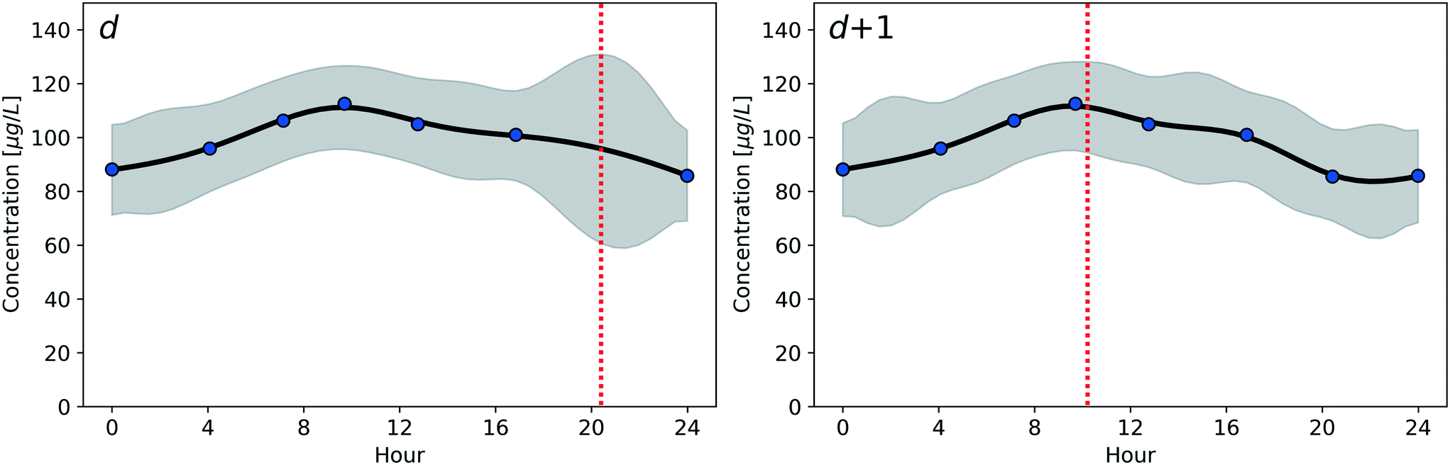Fig. 1 Example of sampling time selection in two consecutive sampling days for an algorithm targeting the maximum daily concentration. The black line and the grey area represent respectively the mean and confidence bounds estimated by the GP implemented in both algorithms. The red vertical dashed line shows the selected sampling instant at the given day, while the blue dots represent the concentrations in samples collected previously.

To adapt to concentration pattern changes Seq(GP-UCB-SW) trains the GP on the last n days, where n is the length of the sliding window, similar to what has been proposed by Garivier and Moulines.³¹ The pseudo-code for Seq(GP-UCB-SW) is shown in Algorithm S1.†

Seq(GP-UCB-CD), instead, similar to what has been proposed by Liu et al.,³² performs change detection through an online change-point method³⁸ using the non-parametric scale-location Lepage test.³⁹ Such a test, being non-parametric, does not require prior information on the monitored process and allows control of both changes in the variability and the central value of the monitored objective. Furthermore, this change detection test provides already-defined thresholds to limit the occurrence of false positive change detection alarms by controlling the average number of observations (i.e., the number of measured target contaminant concentrations) between two consecutive occurrences (commonly referred to as ARL₀): it was applied either to the measured daily maximum concentration or the measured daily maximum, daily minimum, and daily maximum variation, depending on the monitoring objective. Seq(GP-UCB-CD) requires an initial training period (TW), during which the samples are assumed as independent and identically distributed, to let the GP learn the daily pattern appropriately and correctly identify the instant to sample before starting the detection of target value changes. To favour the detection of changes occurring throughout the whole day, after each sampling event Seq(GP-UCB-CD) randomly selects the next sampling instant with probability α, called exploration percentage. Note that, due to the self-starting capabilities of Seq(GP-UCB-CD), before detecting any change, it requires a minimum number of observations after the initial TW which are assumed without pattern changes. The pseudo-code for Seq(GP-UCB-CD) is shown in Algorithm S2.†

Notice that both Seq(GP-UCB-SW) and Seq(GP-UCB-CD) provide an unbiased estimate of the maximum (or maximum and minimum) contaminant concentrations and temporal location. Such estimates are obtained for each monitoring day through a Monte Carlo approach drawing 100 GP realizations to estimate the probability that each time instant corresponds to the maximum (or minimum) contaminant concentration and using those probabilities to perform a weighted average over the concentrations used to train the GP, similar to what was proposed by D'Eramo et al.⁴⁰

2.2 Performance evaluation metrics

Two different conflicting metrics have been used to evaluate the effectiveness of the monitoring strategies employed.

The first performance metric is the relative difference between the target values observed by a monitoring scheme and their true values occurring each day (RDOT). Formally:

RDOT = (v_obs − v_true)/v_true,

where v_obs is the value observed for the quantity analysed by a monitoring scheme during a given day, and v_true is the true value for the corresponding quantity in the same day. In our modelling, we either analyse the maximum concentration or the maximum concentration variation of a target contaminant, obtaining respectively RDOT_max and RDOT_delta. Such a metric allows testing the error performed by the monitoring schemes to identify the appropriate sampling instants: the closer to zero the RDOT value, the lower the difference between the observed and the true target value, and the better the performance of the selected monitoring strategy.

The second metric is the number of samples per day, namely SPD [day⁻¹], requested by the monitoring scheme. Such a metric is used as a proxy for the operating costs due to both reagents used for the sample analyses and instrument maintenance. Therefore, the smaller the number of samples requested, the better the algorithm performs in terms of operational costs, but, in general, the worse the estimation task is fulfilled.

2.3 Case studies

The proposed algorithms were tested on: (i) two synthetic scenarios, derived from high-frequency monitoring campaigns of full-scale drinking water distribution systems, and (ii) a scenario employing real-world data directly collected from an automatic instrument installed in a distribution system. These scenarios were selected to test daily concentration patterns and daily pattern changes linked with different water contaminants (chemical and microbiological) and characterized by various degrees of complexity. In fact, the synthetic scenarios allowed realistic concentration patterns and pattern changes to be assessed in a controlled manner. Meanwhile, the real-world scenario provided the opportunity for an evaluation characterized with a higher degree of complexity and pattern stochasticity. While the algorithms' parameters were changed between experiments, ARL₀ was set to the constant value of 500. Alongside the proposed algorithms, two common traditional monitoring schemes have been employed for comparison: fixed-time and random sampling.^41,42 Both schemes were tested by varying the number of samples per day n ∈ {2, 3, 4, 5, 6}. Under fixed-time sampling, a fixed number of equally spaced instants are sampled each day. For each number of samples per day, all the possible combinations of sampling instants were tested. Meanwhile, random sampling consists of randomly (with uniform probability) selecting a fixed number of instants each day.

2.3.1 Synthetic scenarios. Both synthetic scenarios simulated contaminant concentrations for 180 days by stochastically perturbing, with a given uncertainty, the daily concentration patterns retrieved from full-scale monitoring studies and imposing a variation of the daily pattern after a selected period. In both scenarios,⁴⁸ equally distributed sampling instants (one every 30 minutes over the day) were considered, randomly selecting the starting sample between 7:00 and 16:00, considered as plausible working hours. As the data of each simulation day was generated randomly, the performances of all monitoring strategies were averaged over 100 independent simulations.

The first scenario was derived from the hourly Intact Cell Count (ICC) measurements provided by Nescerescka et al.⁴³ The measured pattern shows a constant baseline concentration with two short-lived ICC peaks which were modelled using a constant baseline and two Gaussian-shaped peaks (Fig. S1†). An uncertainty equal to the analytical uncertainty specified by the authors of the study was used to introduce stochasticity in the simulated patterns. An abrupt shift of 1 h in the occurrence of the ICC peaks was manually imposed on the daily pattern after 90 simulation days to mimic a possible change caused by variations in the pump scheduling, water demands or drinking water treatment plant operations^3,11,21 (Fig. S1†). In this scenario, the monitoring schemes were evaluated targeting the maximum variation in terms of concentration, as the ICC is not linked to consequences on human health⁴⁴ and legislations often focus purely on its variations.¹⁹ This scenario can be considered as representative of real-world involving complex daily concentrations patterns, presenting rapid concentration variations, multiple contaminant peaks throughout the day and abrupt pattern changes. Such characteristics occur commonly in microbiological concentrations in drinking water due to treatment plant management changes and peaks in water demands.^{3,4,6,11,12,43}

In the second synthetic scenario, trihalomethanes (THMs) are considered as the target contaminant. The stochastic daily concentration pattern used in this scenario was generated based on the model formulated by Chaib and Moscandreas,⁹ derived from 7 weeks of THM analyses performed every 4 hours in a full-scale system. This daily pattern presents a continuous variation of the THM concentration throughout the day with a single broad peak around midday (Fig. S2†). Stochasticity in the daily concentration pattern was obtained considering both the uncertainty regarding the amplitude of the daily THM fluctuations and their periodicity, as indicated in the original study. Furthermore, a gradual seasonal change in the daily pattern shape was simulated by shifting the THM concentration peak gradually by 6 h between the 70th and 120th simulation days in accordance with the seasonal differences found in Wang et al.⁴⁵ (Fig. S2†). Due to the presence of a legislative maximum allowed for THM concentrations and the presence of a direct human health risk,^46,47 in this scenario the monitoring schemes were evaluated for the identification of the sampling instant revealing the maximum concentration. This latter scenario, characterized by more gradual concentration changes, can be considered representative of simple contaminant concentration patterns resulting from the variation of environmental conditions (e.g., temperature, light).^7,9,45

2.3.2 Real-world scenario. The algorithms have also been tested using the real-world data presented by Gabrielli et al.⁶ In brief, total cell counts were measured in a non-chlorinated drinking water distribution system with a bi-hourly frequency for around 5 months (from May to October) with an online flow-cytometer (Fig. S3†). As highlighted in the mentioned paper, the dataset presents an overall increase in total cell counts during the central summer months (July and August) and different daily patterns during the monitored period. The dataset presents few gaps due to technical issues that occurred during the monitoring campaign. In our simulations, such gaps have been ignored, directly linking the last day before their occurrence to the first day after the restart of the measurements, mimicking what would be observed by an unattended automatic algorithm in case a malfunctioning of the online instrument occurs. As for the previous microbiological scenario, the algorithms have been evaluated on the identification of the concentration variations. Similar to what was done for the synthetic datasets, the algorithm performances have been averaged over 100 simulations where the starting sample was chosen randomly between the ones in the first monitoring day.

2.4 Data and code availability

The implementation of both Seq(GP-UCB-SW) and Seq(GP-UCB-CD), together with the code used to simulate the synthetic scenarios and a test script, is publicly available at: https://github.com/mgabriell1/SeqMAB-environmental-monitoring. The algorithms and synthetic scenarios have been implemented in Python (https://www.python.org/), using the libraries Numpy,⁴⁸ pandas,⁴⁹ Matplotlib⁵⁰ and Scikit-learn.⁵¹ The change detection test was based on the R package cpm,⁵² which was integrated into the Python script through the rpy2 library (https://rpy2.github.io/).

3 Results

3.1 Performance comparison against the traditional monitoring scheme

3.1.1 Synthetic scenarios. Firstly, both the proposed algorithms and the traditional monitoring schemes have been tested on the two synthetic scenarios, as shown in Fig. 2 and 3. Fig. 2 presents the average performance of the tested monitoring schemes in the identification of the sampling instants connected to maximum and minimum concentrations (RDOT_delta) in the ICC synthetic scenario, which shows an abrupt pattern change mimicking the effects of either variations in the drinking water management strategies or water demand patterns. In general, it is possible to observe the trade-off between the two metrics chosen: an increase of the RDOT_delta value is generally achievable analysing a larger number of samples. Noticeably, since fixed-time sampling requires the manual selection of a given number of time instants per day at each SPD (e.g., for SPD = 2 d⁻¹: 1 AM and 1 PM, or 2 AM and 2 PM, and so on), multiple combinations are possible. As shown by the difference between the RDOT_delta of the best, median and worst sampling time instant combinations at each SPD value, each combination provides different performances. Such an issue is particularly evident in the case of low sampling frequencies (i.e., in our case lower than 6 samples per day), where coincidentally the number of possible sampling instant combinations increases. As indicated by the arrows' length, the RDOT_delta of fixed-time sampling varies greatly between before and after the pattern change (up to 5 times approximately). Compared to fixed-time sampling, random sampling offers an average RDOT_delta which, however, does not vary before and after the pattern change. The two proposed algorithms achieve a RDOT_delta, which would be obtained by random sampling only with SPD > 6 d⁻¹ and is matched only temporarily (i.e., before or after the pattern change) by fixed-time sampling instant combinations. Indeed, only one fixed-time sampling instant combination with SPD = 6 d⁻¹ provides a comparable estimate of the daily concentration variation throughout the whole simulation, although requiring more than twice the number of samples per day. Both algorithms successfully adapt to the pattern change, showing no difference in both SPD and RDOT_delta values before and after the pattern change. Seq(GP-UCB-CD), in addition, correctly identifies the time of its occurrence (Fig. S4†).

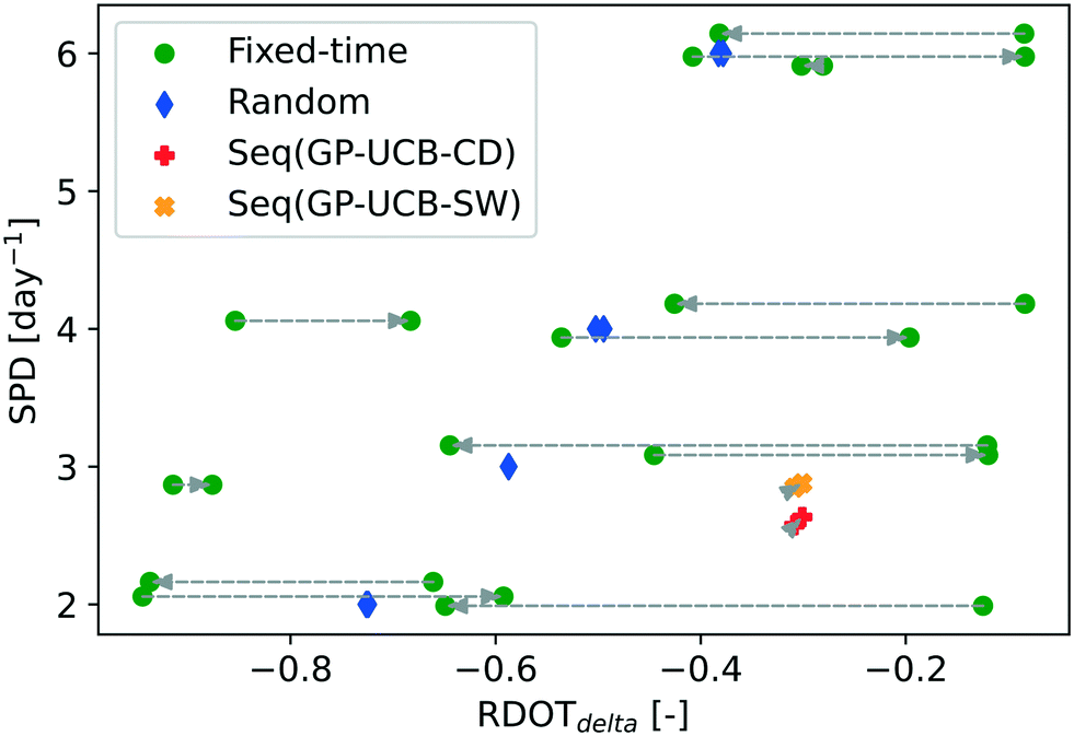Fig. 2 Average performances of tested monitoring schemes on the ICC synthetic scenario before and after the pattern change. For each monitoring scheme, an arrow connects the points indicating the performances before and after the pattern change, pointing toward the one representing the performances after the pattern change. Regarding fixed-time sampling, for each SPD value, only the sampling instant combinations which achieve the worst, median and best performances before the pattern change have been shown and jitter was applied in order to reduce overlapping. The proposed algorithms' results have been obtained with the following algorithm parameterization: SW = 30 d, TW = 30 d, α = 0.075.

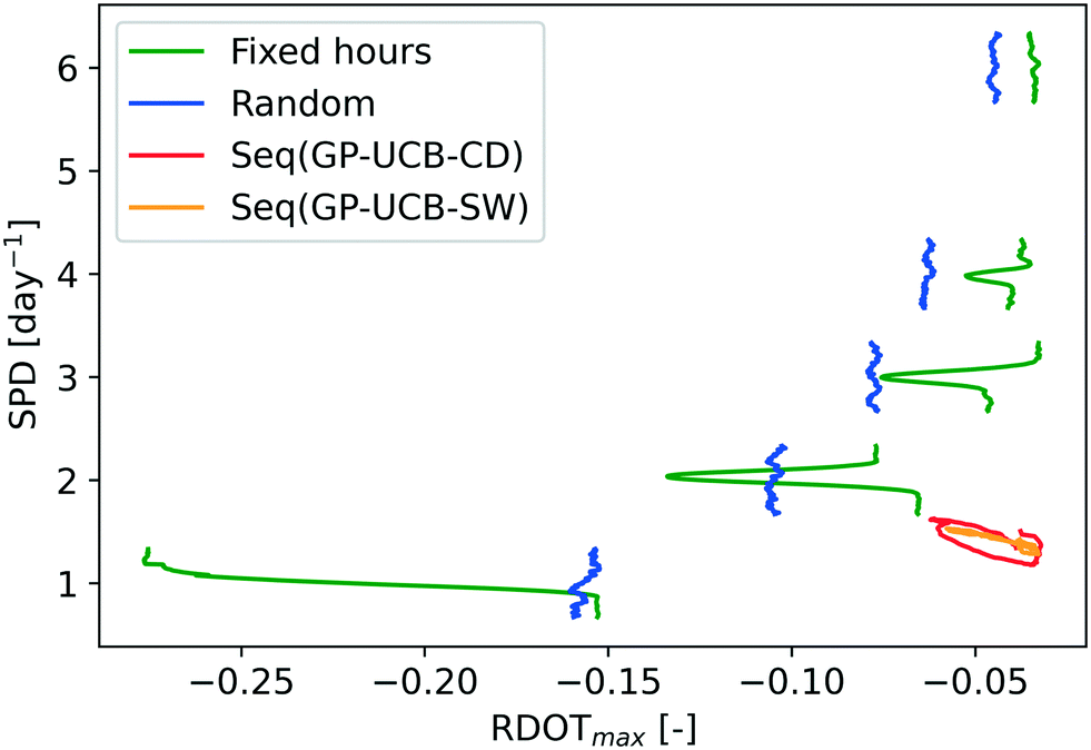Fig. 3 Average performances of tested monitoring schemes along the THM synthetic scenario (rolling mean, n = 25). To show the temporal variation of the RDOT_max obtained by the traditional schemes along the gradual pattern change a vertical displacement was applied at each SPD value. For each SPD value, the temporal RDOT_max evolution is to be read vertically moving from the lower to the higher SPD values. To avoid clutter only the fixed-time sampling instant combination with median performances before the pattern change was shown. The proposed algorithms' results were obtained with the following algorithm parameterization: SW = 30 d, TW = 30 d, α = 0.1.

Similar to Fig. 2, the results obtained in the THM synthetic scenario are shown in Fig. 3 and S5 and S6,† with the RDOT being evaluated against the maximum daily concentration (RDOT_max). Different from the previous synthetic scenario, the daily THM pattern is subjected to a gradual change, representing a possible seasonality⁴⁵ and, for this reason, the evolution of the evaluation metrics obtained by each monitoring scheme during the whole period is shown. In general, compared to the previous scenario, a higher RDOT (i.e. a more accurate estimate of the target value) is achieved by all monitoring schemes. In addition, fixed-time sampling instant combinations at higher SPD values show a reduced variation of the RDOT_max values throughout the simulations, due to the broadness of the concentration peak. However, the results of this scenario agree with what has been observed previously: (i) the performance of the traditional monitoring schemes increases with larger SPD values, (ii) random sampling provides average performances, but is resilient to pattern changes and (iii) fixed-time sampling, RDOT_max is not resilient to pattern dynamicity and presents performances which vary significantly among different sampling instant combinations (Fig. S5 and S6†). The proposed algorithms obtain very similar performances in terms of both RDOT_max and SPD values, resulting in a RDOT_max which is matched by traditional schemes only using more than two times the number of samples per day. It is possible to see how, during the gradual pattern change, both algorithms suffer from a slight decrease in RDOT_max and increase temporarily their SPD in order to readapt the pattern estimate performed by the GP to the new pattern. However, while Seq(GP-UCB-SW) results in a smooth change of RDOT_max and SPD values during the simulation, Seq(GP-UCB-CD) adapts to the gradual change only after detecting its presence (Fig. S7†), resulting in a stepwise adaptation to the pattern change.

3.1.2 Real-world scenario. The results of the monitoring scheme performances targeting the maximum concentration variation in the real-world scenario, over the entire monitoring period, are shown in Fig. 4 and 5. While Fig. 4 displays the RDOT_delta obtained by the proposed algorithms and the traditional monitoring schemes allowing its fluctuations to be observed, Fig. 5 focuses on the trade-off between SPD and RDOT_delta values, showing their average computed over the whole monitoring period. Similar to what has been observed for the two synthetic scenarios, both traditional monitoring schemes obtain better performances at the expense of higher SPD values, with random sampling showing stable RDOT_delta and fixed-time sampling resulting in large variations of its value as observed, for example, between day 50 and 100 (Fig. 4), in which the concentration pattern changes dramatically (Fig. S3†) likely due to a variation in the water consumption caused by the onset of summer vacations.⁶ Finally, also the presence of large performance differences between fixed-time sampling combinations is confirmed, as indicated by the broad gap between the best, median and worst sampling combinations. The RDOT_delta of both developed algorithms, instead, while still fluctuating more than random sampling, shows in most cases smaller variations compared to fixed-time sampling (Fig. 4). Except for the monitoring schemes with SPD = 6 d⁻¹, the average RDOT_delta of Seq(GP-UCB-SW) and Seq(GP-UCB-CD) is outperformed significantly by only the best combination of fixed-time sampling (Fig. 5), despite both algorithms selecting only around 2.7 samples per day. However, without a priori information, the chance of selecting such best-performing fixed-time sampling instant combination is only 16%, 25%, and 33%, considering respectively 2, 3, and 4 samples per day. Indeed, considering the sampling combinations with the median performance for each SPD value as representative of the fixed-time monitoring performance in case of no a priori information, it is possible to note how traditional monitoring schemes are Pareto-dominated by the proposed algorithms, i.e. they have worse characteristics on all the performance metrics analysed. Actually, neither median fixed-time nor random sampling can provide a RDOT_delta comparable to the one displayed by the proposed algorithms with a similar SPD, as such performances are achievable only at the expense of a higher SPD, highlighting the potential of the proposed algorithms to handle complex daily patterns and their dynamics.

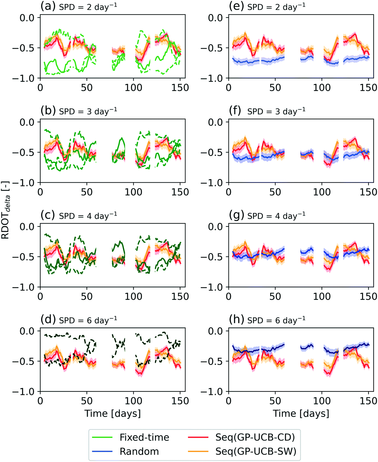Fig. 4 Comparison of the average RDOT_delta obtained in the real-world scenario (rolling mean, n = 10) obtained by Seq(GP-UCB-SW), Seq(GP-UCB-CD), and the traditional schemes for different SPD values: the performance of fixed-time is shown in subplots (a)–(d), while that of random sampling in subplots (e)–(h). Seq(GP-UCB-CD) and Seq(GP-UCB-SW) results have been shown in all subplots to aid the visual comparison with traditional strategies. Only the fixed-time sampling combinations with overall maximum, minimum (dashed line) and median (solid line) RDOT_delta have been shown to avoid excessive clutter. The proposed algorithms' results have been obtained with the following algorithm parameterization: SW = 15 d, TW = 20 d, α = 0.075.

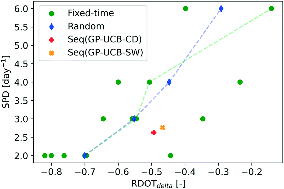Fig. 5 Average performances obtained by the proposed algorithms and the traditional schemes over the entire monitoring period in the real-world scenario. Regarding fixed-time sampling, multiple performances at each SPD value refer to the several sampling instant combinations tested. The dashed green and blue lines connect, respectively, the dots representing fixed-time sampling instant combinations with the median RDOT_delta and random sampling. Mean confidence bars are not reported as negligible. The proposed algorithms' results were obtained with the following algorithm parametrization: SW = 15 d, TW = 20 d, α = 0.075.

Focusing exclusively on the two proposed algorithms, the sliding window approach implemented in Seq(GP-UCB-SW) achieved a higher RDOT_delta (approximately 7%) than the active change detection test adopted by Seq(GP-UCB-CD), employing on average only 19.5 more samples over the entire 5-months period. On the other hand, Seq(GP-UCB-CD) provides pattern change alerts, detecting in most simulations their occurrence (Fig. S8†) before and after the monitoring gaps, as confirmed by the inspection of the full original dataset (Fig. S3†).

3.2 Sensitivity analysis

The robustness of the performance of the proposed algorithms was tested by varying the values of the parameters to assess the effect of a suboptimal parameterization, both in the synthetic and the real-world scenarios. Table 1 presents the mean RDOT values obtained with different parameter combinations tested in the two synthetic scenarios.

Table 1 Mean RDOT_delta and RDOT_max obtained by the proposed algorithms in the ICC and THM synthetic scenarios as a function of the parameters' values. Mean 95% confidence intervals are included in brackets

	Seq(GP-UCB-SW)				Seq(GP-UCB-CD)
	SW = 10 d	SW = 15 d	SW = 30 d		TW = 10 d	TW = 30 d
ICC scenario	−0.575 (0.005)	−0.453 (0.006)	−0.337 (0.006)	α = 0.05	−0.235 (0.007)	−0.223 (0.007)
				α = 0.075	−0.250 (0.009)	−0.236 (0.007)
				α = 0.15	−0.297 (0.007)	−0.284 (0.007)
THM scenario	−0.055 (0.001)	−0.053 (9 × 10^−4)	−0.058 (0.001)	α = 0.05	−0.049 (9 × 10^−4)	−0.048 (8 × 10^−4)
				α = 0.075	−0.049 (9 × 10^−4)	−0.048 (8 × 10^−4)
				α = 0.15	−0.051 (0.001)	−0.051 (9 × 10^−9)

---

Focusing on the results of Seq(GP-UCB-SW), we can see how a significantly different behaviour exists in the two scenarios, as such scenarios represent pattern changes with different complexities and change types. In fact, the performance of Seq(GP-UCB-SW) continues to increase as the sliding window length increases in the ICC scenario, while such performance peaks with a sliding window equal to 15 days in the THM scenario.

About Seq(GP-UCB-CD), short training windows reduce the obtained RDOT, since they affect the estimation of the pattern shape leading to an increased presence of false-positive change detection (Fig. S9†). Similar to what has been observed for Seq(GP-UCB-SW), this effect is less evident for the THM scenario, due to its lower complexity. Instead, an increase in the values of α is connected to worse performances, as Seq(GP-UCB-CD) will choose more frequently a sampling instant not connected to either maximum or minimum concentrations.

The sensitivity analysis of the algorithm parameters in the real-world scenario is shown in Fig. 6. As discussed beforehand, an excessive or an overly short Seq(GP-UCB-SW) sliding window length impacts both the RDOT_delta achieved and the number of samples per day analysed. Regarding Seq(GP-UCB-CD), an excessively long training window TW results in decreased performances, as different patterns might be included in this window. In addition, as no change detection is performed during this initial period, an excessive training period will also limit the possibility to detect changes and adapt accordingly. As already noted, a clear decrease in the average RDOT_delta is obtained in the case of an excessively large α value. However, an appropriate percentage of exploratory samples is needed to improve the worst-case performance of the algorithm and to properly control the concentration throughout the whole day. Indeed, while the difference between the average RDOT_delta with α equal to 0.05 and 0.075 is small due to the limited α variation, the worst-case performance, represented by the 5th quantile, shows a larger difference (i.e., −0.56 with TW = 20 d and α = 0.05; −0.54 with TW = 20 d and α = 0.075).

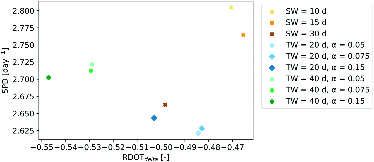Fig. 6 Variation of RDOT_delta and SPD values obtained by Seq(GP-UCB-SW) and Seq(GP-UCB-CD) in the real-world scenario, due to different sliding window (SW) or training window (TW) lengths and exploration percentage (α) values.

4 Discussion

4.1 Monitoring scheme performances

In general, both synthetic and real-world scenarios highlight how to obtain a RDOT closer to zero, indicating a better characterization of maximum and/or minimum concentrations (see section 2.2), and SPD values should generically be increased, leading to higher operating costs. In any case, other than just the monitoring frequency, the importance of the selection of the sampling instants is critical to properly monitor daily contaminant concentration patterns. As it can be observed by comparing the results of the two synthetic scenarios, this is especially true in case the monitoring target is the maximum daily concertation variation, and complex patterns with high concentration variability and impulse-like contaminant peaks are present.

Selecting every possible time instants with equal probability, as done by random sampling, provides an estimate of the target values resilient to pattern changes; anyway, it does not allow their true value to be properly characterized, as noted by Gabrielli et al.⁶ and highlighted by the mediocre RDOT values in Fig. 2–5. In practical terms, although changes in target contaminant concentrations are detected by a monitoring scheme implementing the random sampling, looking at the average values of the analysed samples, it is not possible to accurately observe the contaminants' target value every day. Consequently, erroneous evaluations of the process stability and water quality could be drawn, for example, regarding the temporal stability of ICC concentrations affected by treatment or distribution.³

Focusing exclusively on selected sampling instants and neglecting the others, as done by fixed-time sampling, might lead to the true target contaminant concentration being missed, due to: (i) misspecified sampling instants (e.g., fixed-time sampling instant combinations with poor performances both before and after the pattern change in Fig. 3), or (ii) inconclusive information on the observed variation which cannot be attributed to a change in the maximum and minimum daily concentrations or just to a change in the time of their occurrence (e.g. fixed-time sampling is unable to catch the shift of the maximum THM concentrations due to differences in water retention times and temperature profiles as in Fig. 3 and S2, S5 and S6†).^9,45 Such erroneous evaluations might result in inadequate, or even harmful, interventions. For example, erroneously-observed reductions in THMs, as highlighted in Fig. 3, might lead drinking water treatment plant managers to relax the treatment steps dedicated to their removal, potentially increasing consumers health risk. Similar results could occur in case of increases in THM concentrations at times different from the ones sampled and which might go undetected. In fact, selecting a sampling combination with the best performance during one period (e.g., selected using a preliminary sampling campaign as proposed by Gabrielli et al.⁶) does not solve this problem, as daily patterns might change unpredictably. Furthermore, these issues are particularly relevant when employing low sampling frequencies (i.e., in our scenarios SPD < 6 d⁻¹), as the increasing number of possible sampling instant combinations reduces the probability of selecting the best combination without a priori information.

The proposed algorithms, instead, actively make use of the collected samples to select the successive sampling instants, resulting in performances resilient to pattern changes, but ensuring lower operating costs (with SPD being a proxy, see section 2.2). For example, comparable RDOT could be achieved only by more than two times higher SPD values (i.e., operating costs) in the scenarios investigated. Noteworthily, such performances are obtained without any a priori or external information on the monitoring process, removing the need for explicit human intervention. In case of pattern changes, their performance will temporarily drop, as shown in Fig. 3 and 4, but with a limited number of samples the new pattern would be successfully learned, resulting in again high performances which, in the tested scenario, allow the total cell concentration to be effectively monitored and anomalous variations to be properly assessed, which could have been missed otherwise. Comparing the two algorithms, the better RDOT_delta obtained by Seq(GP-UCB-SW) in the real-world scenario highlights the flexibility of the sliding window approach for the adaptation to generic changes in the data.⁵³ In fact, active approaches, as the one used by Seq(GP-UCB-CD), are usually not well suited for gradual or complex pattern changes and can possibly lead to a significant delay before the change detection and the subsequent adaptation.³⁸ However, such loss in RDOT_delta is compensated for by the ability to actively detect changes in the daily concentration pattern and to provide alerts (e.g., Fig. S8†), which could trigger additional investigations to reveal the cause of the change, aiding the management of the infrastructure. Nonetheless one must take care to avoid an excessive number of false alarms, as such events could be problematic for water utilities and environmental protection agencies both due to the costs for the verification of the change origin and the decrease of the trust in the events' detection.⁵⁴

4.2 Algorithm parameter selection guide

Based on the results of the sensitivity analysis, some guidance for the application of the proposed algorithms can be obtained. It should be stressed that the best algorithms' parametrization depends on both the daily pattern complexity and its type of change. In any case, by comparing x-axis scales of the real-world scenario results in Fig. 5 and 6, it is possible to note the robustness of these algorithms to the use of suboptimal parameter values, as even the worst parameterization tested still outperforms the median performances of the traditional schemes. Since theoretical results regarding the optimal sliding window length cannot be used in real-world environmental monitoring application,³³ based on the results of the real-world sensitivity analysis, we suggest the use of a sliding window of limited length. While such a setting will lead to a slight increase in monitoring costs due to the larger number of samples per day analysed, such an option allows more intense sampling of the entire set of sampling instants and faster adaptation of the monitoring scheme to pattern changes. In fact, a shorter-than-optimal sliding window achieved a higher RDOT_delta than using one of excessive length, as this latter option can lead to the inclusion of samples which do not represent the current pattern, especially in gradual (e.g., seasonal) changes,⁵³ as simulated in the THM scenario. Beware that excessively short sliding windows might still hamper performances, as they would not allow Seq(GP-UCB-SW) to effectively learn the daily pattern, as highlighted by the length required to improve RDOT_delta in the ICC scenario.

The training window length TW must be set accordingly to the complexity of the daily pattern expected in order to allow the Seq(GP-UCB-CD) algorithm to properly learn the pattern and avoid excessive false positive alarms, as highlighted by the sensitivity analysis on the ICC scenario. It should be stressed that any operation which might affect the monitored contaminant or its pattern should be avoided during this period (e.g., change filters and/or its backwash schedule), since uncontrolled conditions during the initial training might limit the algorithm's ability to learn the water quality pattern and the change detection performances.³⁸

The value of α should reflect the degree of stochasticity in the pattern occurrence and should not be set too small to prevent excessively low worst-case performances. Hypothetically, if the time instants of the maximum (and minimum) concentration were known to be fixed, the best performances would be obtained with α = 0. On the other hand, in the case of a completely random concentration pattern, the most appropriate value should be 1, as no single time instant could be considered as having the maximum (or minimum) concentrations. Such consideration explains the different results of the sensitivity analysis conducted on α: the optimal value of α lies below 0.05 in the synthetic scenarios due to their lower pattern stochasticity (i.e., the best sampling locations are more repetitive due to the simpler pattern changes) (Table 1), while to properly account the real-world data stochasticity a value of 0.075 is needed (Fig. 6).

Regarding the choice between the two algorithms, in our opinion, Seq(GP-UCB-SW) is more suited when complex pattern dynamicity might be present, or in the case where it is not possible to provide controlled conditions during the initial Seq(GP-UCB-CD) training phase due to its continuous pattern adaptation. Furthermore, the misspecification of the sliding window length appears to affect less Seq(GP-UCB-SW) performances, compared to the use of suboptimal parameters for change detection. On the other hand, Seq(GP-UCB-CD) is more suited in the case of more controlled situations, e.g., in drinking water treatment plants, where deviations from the normal conditions must be actively identified and notified as soon as possible to minimize possible negative outcomes (e.g., the distribution of contaminated water).

In any case, basic knowledge of the concentration pattern which is expected aids the algorithm parametrization. In general, changes in the environmental conditions (e.g., day/night cycles) generically lead to smooth and simple concentration patterns of chemical contaminants (e.g., THM scenario, Wang et al.⁴⁵), which likely vary gradually throughout the year, thus requiring shorter sliding and training windows. On the other hand, concentrations of microorganisms and of chemicals linked with intermittent human activities (e.g., ICC and real-world scenarios, Besmer and Hammes,³ Favere et al.,¹¹ Buysschaert et al.¹²) can result in complex patterns (i.e., presenting drastic daily fluctuations), which might also change abruptly (e.g., within a few days), requiring the use of longer sliding and training windows. A general indication on the best algorithms and suggested parameters' values as a function of the target value, pattern complexity and change type can be found in Table 2. The parameter values need to be considered as a general indication, which needs to be adapted to the characteristics of each specific case study. In particular, in the case of high pattern stochasticity, the value of the sliding window of Seq(GP-UCB-SW) should be slightly decreased, i.e. by 2–3 days, in order to sample more often all the possible sampling instants. The same effect can be obtained in Seq(GP-UCB-CD) by increasing the value of α, i.e. 0.025–0.05. To obtain the best-performing and case-specific parameter values, it is advised to test the algorithms' performances using different parametrizations on synthetically generated time series based on historical data.

Table 2 Summary of the best algorithms and suggested parameter values for different scenarios

Target value	Pattern complexity	Pattern change type	Algorithm	Suggested parameters' values
Max concentration	Simple	Abrupt	Seq(GP-UCB-CD)	TW = 10 d
				α = 0.05
		Gradual	Seq(GP-UCB-SW)	SW = 10 d
	Complex	Abrupt	Seq(GP-UCB-CD)	TW = 17 d
				α = 0.075
		Gradual	Seq(GP-UCB-SW)	SW = 15 d
Max concentration variation	Simple	Abrupt	Seq(GP-UCB-CD)	TW = 15 d
				α = 0.05
		Gradual	Seq(GP-UCB-SW)	SW = 13 d
	Complex	Abrupt	Seq(GP-UCB-CD)	TW = 20 d
				α = 0.075
		Gradual	Seq(GP-UCB-SW)	SW = 17 d

---

4.3 Extension of the applicability of developed algorithms

While all case studies here tested derive from drinking water, daily contaminant concentration patterns comparable to the tested scenarios can also be found in surface water and wastewater for several contaminants, due to the cyclic nature of anthropic activities,⁵⁵ environmental conditions (e.g., light intensity, temperature), and other affecting characteristics.⁵⁶ For example, contaminants in surface water and both treated and untreated wastewaters can be highly affected by variations in environmental conditions (e.g., some metals, nitrogen-species, photolabile compounds and microbiological indicators are affected by diurnal light intensity variation^7,57,58), impulse-like contaminant releases, especially in small catchments,^15,50 and daily changes during wastewater treatment.^14,17,59,60 For this reason, traditional sampling schemes might not be appropriate, while the use of the proposed algorithms could be beneficial, allowing the presence of unexpected concentrations to be identified, which could warrant further investigation.

As other water matrices might be more affected by environmental conditions, the developed algorithms could be extended to include the use of external information to handle their aperiodic effects. In case a triggering event is known to affect the concentration of the monitored contaminant, Seq(GP-UCB-SW) or Seq(GP-UCB-CD) could be coupled with event-based sampling.^20,41 In such a case, the proposed algorithms would indicate the sampling times during normal conditions (e.g., dry weather), while external information could trigger a threshold for event-based sampling (e.g., rainfall), possibly still calibrated using MAB strategies. In other cases, where a triggering event is not easily identifiable, a possible alternative is the use of contextual bandit techniques,⁶¹ which infer the relationship between external information (e.g., meteorological conditions and/or other easily-monitorable water parameters) and the targeted contaminant concentration.

In any case, even though Seq(GP-UCB-SW) and Seq(GP-UCB-CD) have been developed to tackle the presence of daily contaminant concentration patterns, they can also be used when no apparent pattern is present (yet) and adapt to its onset, regardless of the water matrix. In such a case, Seq(GP-UCB-SW) results in a mostly uniform sampling of all the available sampling instants (Fig. S10†). On the other hand, Seq(GP-UCB-CD) focuses most of the samples on a single sampling instant, exploring the remaining ones based on the specified α (Fig. S11†).

4.4 Adapting the developed algorithms to manual and low-frequency monitoring

The proposed algorithms are not usable only when applied to online automatic instrumentation, but also in other scenarios. The same procedure can be performed with lower time frequencies, e.g., taking samples only once per week, without any modification to the algorithms. In fact, the only difference is the time required by the algorithms to learn the pattern's shape and, in the case of Seq(GP-UCB-CD), the time needed to detect its changes. In addition, one may adopt delayed bandit techniques, if a significant delay in the analyses is present.⁶²

Regarding manual sampling, as already noted by Ekklesia et al.,⁶³ sampling in the same location more than once per day might not be practical. For monitoring campaigns targeting the maximum variability, a practical workaround is to sample the time instant corresponding to the maximum concentration at a given day and wait for the next sampling day to sample the time instant corresponding to the minimum. Finally, it is worth noticing that, as routine manual sampling is restricted to working hours (e.g., 8:00–17:00), no information can be obtained for the rest of the day, possibly neglecting relevant events. Autosamplers, instead, can be programmed to collect samples at any time of the day for multiple days.⁶⁴ However, the analysis is performed only later, limiting the update of the algorithms. For this reason, the frequency of the analysis of the collected samples needs to be adjusted to avoid errors due to the use of outdated information. While autosamplers could also be used to collect composite samples, the use of this technique would lead to the collection of averaged concentrations without the possibility to identify short-lived concentration peaks.¹⁴

Finally, it can be of interest to monitor at the same time different contaminants possibly characterized by different best sampling times (e.g., different concentration peak times). As the algorithms have been designed to focus on a single contaminant (either as a single compound or as a sum of compounds from the same chemical family, e.g., THMs), two options are available depending on the aim of the monitoring campaign. In case the concentration of every single contaminant is of interest, the solution would be to use one algorithm for each contaminant and take a sample every time it is suggested by any of the algorithms. Even though in each sample the target value is expected only for a few, or even only one, of the monitored contaminants, it is advisable to carry out the analysis of the entire set of monitored contaminants in each sample. In fact. This aids the estimation of the daily concentration patterns of all the targeted contaminants, resulting in a quicker identification of the best sampling instants and, overall, a lower number of samples analysed. To further reduce monitoring costs linked with the use of different analytical instrumentation, it could be possible to limit the analyses to only the contaminants requiring the same analytical method as the one expected at its target value. The other option consists in the use of the developed algorithms based on an aggregated index estimated from the concentrations of the contaminants of interest. While the sampling instants selected will likely not be characterized by the target concentration of any specific contaminant, such a strategy would be suitable for monitoring campaigns focused on properties which arise from mixtures of contaminants as, for example, the cumulative risk.

5 Conclusions

The results of this work have demonstrated how the use of online learning algorithms permits temporal monitoring schemes to be designed to sample the time instants corresponding to the maximum and minimum concentrations of the target contaminant. In fact, even in the presence of complex daily contaminant concentration patterns, the proposed algorithms are able to better describe contaminant concentrations, while coincidentally analysing less than half the number of samples compared to traditional monitoring schemes. In addition, the monitoring schemes resulting from the application of the proposed algorithms are resilient to daily pattern changes and require no external information or human intervention. The application of these algorithms by water utilities and environmental protection agencies in fast-responding water matrices will benefit not only from more detailed information, which could be used to better understand the effect of technical operations during water treatment or to provide a more accurate estimate of the human or environmental risks, but will also achieve the reduction of the operating costs due to the analyses of the samples, enabling a more widespread water monitoring.

Conflicts of interest

There are no conflicts to declare.

Acknowledgements

The authors would like to thank CAP Holding S.p.A., which manages the integrated water service for the metropolitan area in the outskirt of Milan city, for having funded the Ph.D. grant of Marco Gabrielli, within which this work has been developed.

References

1. World Health Organization, Guidelines for Drinking-water Quality, Fourth.
2. ISO, Water quality — Sampling — Part 1: Guidance on the design of sampling programmes and sampling techniques, ISO, Geneva, Switzerland, 2nd edn, 2006.
3. M. D. Besmer and F. Hammes, Short-term microbial dynamics in a drinking water plant treating groundwater with occasional high microbial loads, Water Res., 2016, 107, 11–18.
4. M. D. Besmer, D. G. Weissbrodt, B. E. Kratochvil, J. A. Sigrist, M. S. Weyland and F. Hammes, The feasibility of automated online flow cytometry for in-situ monitoring of microbial dynamics in aquatic ecosystems, Front. Microbiol., 2014, 5, 265.
5. J. W. Kirchner, X. Feng, C. Neal and A. J. Robson, The fine structure of water-quality dynamics: the(high-frequency) wave of the future, Hydrol. Process., 2004, 18, 1353–1359.
6. M. Gabrielli, A. Turolla and M. Antonelli, Bacterial dynamics in drinking water distribution systems and flow cytometry monitoring scheme optimization, J. Environ. Manage., 2021, 286, 112151.
7. D. A. Nimick, C. H. Gammons and S. R. Parker, Diel biogeochemical processes and their effect on the aqueous chemistry of streams: A review, Chem. Geol., 2011, 283, 3–17.
8. A. W. Brown, P. S. Simone, J. C. York and G. L. Emmert, A device for fully automated on-site process monitoring and control of trihalomethane concentrations in drinking water, Anal. Chim. Acta, 2015, 853, 351–359.
9. E. Chaib and D. Moschandreas, Modeling daily variation of trihalomethane compounds in drinking water system, Houston, Texas, J. Hazard. Mater., 2008, 151, 662–668.
10. J. Favere, B. Buysschaert, N. Boon and B. De Gusseme, Online microbial fingerprinting for quality management of drinking water: Full-scale event detection, Water Res., 2020, 170, 115353.
11. J. Favere, F. Waegenaar, N. Boon and B. De Gusseme, Online microbial monitoring of drinking water: How do different techniques respond to contaminations in practice?, Water Res., 2021, 202, 117387.
12. B. Buysschaert, L. Vermijs, A. Naka, N. Boon and B. De Gusseme, Online flow cytometric monitoring of microbial water quality in a full-scale water treatment plant, npj Clean Water, 2018, 1, 16.
13. P. Stadler, G. Blöschl, W. Vogl, J. Koschelnik, M. Epp, M. Lackner, M. Oismüller, M. Kumpan, L. Nemeth, P. Strauss, R. Sommer, G. Ryzinska-Paier, A. H. Farnleitner and M. Zessner, Real-time monitoring of beta-d-glucuronidase activity in sediment laden streams: A comparison of prototypes, Water Res., 2016, 101, 252–261.
14. M. A. Stravs, C. Stamm, C. Ort and H. Singer, Transportable Automated HRMS Platform “MS2field” Enables Insights into Water-Quality Dynamics in Real Time, Environ. Sci. Technol. Lett., 2021, 8, 373–380.
15. M. Wortberg and J. Kurz, Analytics 4.0: Online wastewater monitoring by GC and HPLC, Anal. Bioanal. Chem., 2019, 411, 6783–6790.
16. A. Ender, N. Goeppert, F. Grimmeisen and N. Goldscheider, Evaluation of β-d-glucuronidase and particle-size distribution for microbiological water quality monitoring in Northern Vietnam, Sci. Total Environ., 2017, 580, 996–1006.
17. A. Hess, C. Baum, K. Schiessl, M. D. Besmer, F. Hammes and E. Morgenroth, Stagnation leads to short-term fluctuations in the effluent water quality of biofilters: A problem for greywater reuse?, Water Res.: X, 2021, 13, 100120.
18. Y. Madrid and Z. P. Zayas, Water sampling: Traditional methods and new approaches in water sampling strategy, TrAC, Trends Anal. Chem., 2007, 26, 293–299.
19. S. Van Nevel, S. Koetzsch, C. R. Proctor, M. D. Besmer, E. I. Prest, J. S. Vrouwenvelder, A. Knezev, N. Boon and F. Hammes, Flow cytometric bacterial cell counts challenge conventional heterotrophic plate counts for routine microbiological drinking water monitoring, Water Res., 2017, 113, 191–206.
20. J.-B. Burnet, M. Habash, M. Hachad, Z. Khanafer, M. Prévost, P. Servais, E. Sylvestre and S. Dorner, Automated Targeted Sampling of Waterborne Pathogens and Microbial Source Tracking Markers Using Near-Real Time Monitoring of Microbiological Water Quality, Water, 2021, 13, 2069.
21. M. D. Besmer, J. Epting, R. M. Page, J. A. Sigrist, P. Huggenberger and F. Hammes, Online flow cytometry reveals microbial dynamics influenced by concurrent natural and operational events in groundwater used for drinking water treatment, Sci. Rep., 2016, 6, 38462.
22. L. Wang, J. von Freyberg, I. van Meerveld, J. Seibert and J. W. Kirchner, What is the best time to take stream isotope samples for event-based model calibration?, J. Hydrol., 2019, 577, 123950.
23. S. Shalev-Shwartz, Online Learning and Online Convex Optimization, FNT in Machine Learning, 2011, vol. 4, pp. 107–194.
24. T. Lattimore and C. Szepesvári, Bandit Algorithms, Cambridge University Press, 1st edn, 2020.
25. S. Pool and J. Seibert, Gauging ungauged catchments – Active learning for the timing of point discharge observations in combination with continuous water level measurements, J. Hydrol., 2021, 598, 126448.
26. S. Russo, M. Lürig, W. Hao, B. Matthews and K. Villez, Active learning for anomaly detection in environmental data, Environ. Model. Softw., 2020, 134, 104869.
27. P. Auer and N. Cesa-Bianchi, Finite-time Analysis of the Multiarmed Bandit Problem, Mach. Learn., 2002, 47, 235–256.
28. E. Kaufman, N. Korda and R. Munos, Thompson sampling: An asymptotically optimal finite-time analysis, in Algorithmic Learning Theory: 23rd International Conference, ALT 2012, Lyon, France, October 29–31, 2012. Proceedings, ed. N. H. Bshouty, G. Stoltz, N. Vayatis and T. Zeugmann, Springer, Berlin, Heidelberg, 2012, vol. 7568.
29. E. Kaufmann, O. Cappe and A. Garivier, On Bayesian Upper Confidence Bounds for Bandit Problems, in Proceedings of the Fifteenth International Conference on Artificial Intelligence and Statistics, ed. N. D. Lawrence and M. Girolami, PMLR, La Palma, Canary Islands, 2012, vol. 22, pp. 592–600.
30. A. Garivier and O. Cappé, The KL-UCB Algorithm for Bounded Stochastic Bandits and Beyond, in Proceedings of the 24th annual conference on learning theory, JMLR Workshop and Conference Proceedings, 2011, pp. 359–376.
31. A. Garivier and E. Moulines, On Upper-Confidence Bound Policies for Switching Bandit Problems, in Algorithmic Learning Theory: 22nd International Conference, ALT 2011, Espoo, Finland, October 5–7, 2011. Proceedings, ed. J. Kivinen, C. Szepesvári, E. Ukkonen and T. Zeugmann, Springer, Berlin Heidelberg, 2011, vol. 6925.
32. F. Liu, J. Lee and N. Shroff, A Change-Detection Based Framework for Piecewise-Stationary Multi-Armed Bandit Problem, in Proceedings of the AAAI Conference on Artificial Intelligence, 2018, vol. 32.
33. F. Trovò, S. Paladino, M. Restelli and N. Gatti, Sliding-Window Thompson Sampling for Non-Stationary Settings, jair, 2020, 68, 311–364.
34. G. Re, F. Chiusano, F. Trovò, D. Carrera, G. Boracchi and M. Restelli, A Change-Detection Based Framework for Piecewise-Stationary Multi-Armed Bandit Problem, in Machine Learning and Knowledge Discovery in Databases. Research Track: European Conference, ECML PKDD 2021, Bilbao, Spain, September 13–17, 2021, Proceedings, Part I, ed. N. Oliver, F. Pérez-Cruz, S. Kramer, J. Read and J. A. Lozano, Springer International Publishing, Cham, 2021, vol. 12975.
35. N. Srinivas, A. Krause, S. M. Kakade and M. Seeger, Gaussian Process Optimization in the Bandit Setting: No Regret and Experimental Design, IEEE Trans. Inf. Theory, 2012, 58, 3250–3265.
36. C. E. Rasmussen and C. K. I. Williams, Gaussian processes for machine learning, MIT Press, Cambridge, Mass, 2006.
37. M. Gabrielli, F. Trovò and M. Antonelli, Adapting Bandit Algorithms for Settings with Sequentially Available Arms, 2021, arXiv:cs/2109.15228.
38. G. J. Ross, D. K. Tasoulis and N. M. Adams, Nonparametric Monitoring of Data Streams for Changes in Location and Scale, Technometrics, 2011, 53, 379–389.
39. Y. Lepage, A combination of Wilcoxon's and Ansari-Bradley's statistics, Biometrika, 1971, 58, 213–217.
40. C. D'Eramo, A. Nuara and M. Restelli, A Change-Detection Based Framework for Piecewise-Stationary Multi-Armed Bandit Problem, in International Conference on Machine Learning, PMLR, 2016, pp. 1032–1040.
41. M. D. Besmer, F. Hammes, J. A. Sigrist and C. Ort, Evaluating Monitoring Strategies to Detect Precipitation-Induced Microbial Contamination Events in Karstic Springs Used for Drinking Water, Front. Microbiol., 2017, 8, 2229.
42. R. A. Skeffington, S. J. Halliday, A. J. Wade, M. J. Bowes and M. Loewenthal, Using high-frequency water quality data to assess sampling strategies for the EU Water Framework Directive, Hydrol. Earth Syst. Sci., 2015, 19, 2491–2504.
43. A. Nescerecka, J. Rubulis, M. Vital, T. Juhna and F. Hammes, Biological Instability in a Chlorinated Drinking Water Distribution Network, PLoS One, 2014, 9, e96354.
44. M. J. Allen, S. C. Edberg and D. J. Reasoner, Heterotrophic plate count bacteria — what is their significance in drinking water?, Int. J. Food Microbiol., 2004, 92, 265–274.
45. L. Wang, Y. Chen, S. Chen, L. Long, Y. Bu, H. Xu, B. Chen and S. Krasner, A one-year long survey of temporal disinfection byproducts variations in a consumer's tap and their removals by a point-of-use facility, Water Res., 2019, 159, 203–213.
46. D. M. DeMarini, A review on the 40th anniversary of the first regulation of drinking water disinfection by-products, Environ. Mol. Mutagen., 2020, 61, 588–601.
47. L. Yang, X. Chen, Q. She, G. Cao, Y. Liu, V. W.-C. Chang and C. Y. Tang, Regulation, formation, exposure, and treatment of disinfection by-products (DBPs) in swimming pool waters: A critical review, Environ. Int., 2018, 121, 1039–1057.
48. C. R. Harris, K. J. Millman, S. J. van der Walt, R. Gommers, P. Virtanen, D. Cournapeau, E. Wieser, J. Taylor, S. Berg, N. J. Smith, R. Kern, M. Picus, S. Hoyer, M. H. van Kerkwijk, M. Brett, A. Haldane, J. F. del Río, M. Wiebe, P. Peterson, P. Gérard-Marchant, K. Sheppard, T. Reddy, W. Weckesser, H. Abbasi, C. Gohlke and T. E. Oliphant, Array programming with NumPy, Nature, 2020, 585, 357–362.
49. W. McKinney, Data Structures for Statistical Computing in Python, in Proceedings of the 9th Python in Science Conference, ed. S. van der Walt and J. Millman, 2010, pp. 56–61.
50. J. D. Hunter, Matplotlib: A 2D graphics environment, Comput. Sci. Eng., 2007, 9, 90–95.
51. F. Pedregosa, G. Varoquaux, A. Gramfort, V. Michel, B. Thirion, O. Grisel, M. Blondel, P. Prettenhofer, R. Weiss, V. Dubourg, J. Vanderplas, A. Passos and D. Cournapeau, Scikit-learn: Machine Learning in Python, J. Mach. Learn Res., 2011, 12, 2825–2830.
52. G. J. Ross, Parametric and Nonparametric Sequential Change Detection in R: The cpm Package, J. Stat. Softw., 2015, 1–20.
53. J. Gama, I. Žliobaitė, A. Bifet, M. Pechenizkiy and A. Bouchachia, A survey on concept drift adaptation, ACM Comput. Surv., 2014, 46, 1–37.
54. J. T. Ripberger, C. L. Silva, H. C. Jenkins-Smith, D. E. Carlson, M. James and K. G. Herron, False Alarms and Missed Events: The Impact and Origins of Perceived Inaccuracy in Tornado Warning Systems: Inaccuracy in Tornado Warning Systems, Risk Anal., 2015, 35, 44–56.
55. C. Song, Z. Qu, N. Blumm and A.-L. Barabási, Limits of Predictability in Human Mobility, Science, 2010, 327, 1018–1021.
56. J. Simonsen and P. Harremoës, Oxygen and pH fluctuations in rivers, Water Res., 1978, 12, 477–489.
57. G. Guillet, J. L. A. Knapp, S. Merel, O. A. Cirpka, P. Grathwohl, C. Zwiener and M. Schwientek, Fate of wastewater contaminants in rivers: Using conservative-tracer based transfer functions to assess reactive transport, Sci. Total Environ., 2019, 656, 1250–1260.
58. E. Traister and S. C. Anisfeld, Variability of Indicator Bacteria at Different Time Scales in the Upper Hoosic River Watershed, Environ. Sci. Technol., 2006, 40, 4990–4995.
59. N. D. Le, X. France, S. Pontvianne, H. Poirot, J. P. Leclerc and M. N. Pons, Daily wastewater pollutant dynamics with respect to catchment population structure, Urban Water J., 2017, 14, 1016–1022.
60. B. G. Plósz, H. Leknes, H. Liltved and K. V. Thomas, Diurnal variations in the occurrence and the fate of hormones and antibiotics in activated sludge wastewater treatment in Oslo, Norway, Sci. Total Environ., 2010, 408, 1915–1924.
61. L. Li, W. Chu, J. Langford and R. E. Schapire, Data Structures for Statistical Computing in Python, in Proceedings of the 19th international conference on World wide web - WWW ‘10, ACM Press, Raleigh, North Carolina, USA, 2010, p. 661.
62. P. Joulani, A. György and C. Szepesvári, Online Learning under Delayed Feedback, in Proceedings of the 30th International Conference on Machine Learning, ed. S. Dasgupta and D. McAllester, PMLR, Atlanta, Georgia, USA, 2013, vol. 28, pp. 1453–1461.
63. E. Ekklesia, P. Shanahan, L. H. C. Chua and H. S. Eikaas, Temporal variation of faecal indicator bacteria in tropical urban storm drains, Water Res., 2015, 68, 171–181.
64. USEPA, Handbook for Sampling and Sample Preservation of Water and Wastewater, Cincinnati OH, USA, 1982.

---

Footnote

† Electronic supplementary information (ESI) available. See DOI: https://doi.org/10.1039/d2ew00089j

---