The bioaccumulation testing strategy for nanomaterials: correlations with particle properties and a meta-analysis of in vitro fish alternatives to in vivo fish tests

Abstract

For manufactured nanomaterials (MNs), given the breadth of forms produced, it is not ethical or practical to test all materials using vertebrates. This study aimed to show how alternative methods could predict the in vivo bioaccumulation potential of MNs in fish. This included exploring the physico-chemical properties of MNs as predictors of bioaccumulation, using the ex vivo gut sac technique to measure total metal uptake, and an in chemico digestibility assay to simulate the bioaccessible metal in the gut lumen of fish. An apparent plateau in net metal accumulation by rainbow trout was evident from data on dietary exposures to CuO nanoparticles (NPs), Ag NPs or Ag₂S NPs in vivo. From the metal concentrations in the tissues compared to the diet, it was possible to derive nano biomagnification factors (nBMFs). The nBMF for the liver showed the best correlations with the physico-chemical parameters, with a significant correlation to the particle dissolution rate (Spearman's correlation, p < 0.01). Moreover, there was a significant relationship between the total metal released in the stomach compartment of the digestibility assay and the total metal concentration in the liver of trout in vivo (Pearson's correlation coefficient, p = 0.02), suggesting the in chemico digestibility assay can predict bioaccumulation potential. The ex vivo gut sac technique also gave good correlations to in vivo results, with r² values between 0.8–0.9. In conclusion, the meta-analyses supports the development of an integrated and tiered approach to bioaccumulation testing that considers the 3Rs (replacement, reduction, refinement) and minimises the use of the fish bioaccumulation test (OECD TG 305), for nanomaterials.

---

Environmental significance

There are currently no steps in the Organisation for Economic Co-operation and Development (OECD) bioaccumulation testing strategy to reliably trigger or waive testing for nanomaterials, or to consider alternatives to using animals. In vitro alternatives include an in chemico digestibility assay and ex vivo gut sacs from fish intestine. A meta-analysis of existing data on these methods was conducted using cupric oxide, silver and silver sulphide nanoparticles. The analysis identified particle metrics as predictors of bioaccumulation potential for nanomaterials in fish. The rapid in vitro alternatives to live fish experiments gave good correlations with the in vivo data. Predictive tools and alternative methods can rationalise nanomaterial testing, with the in vivo fish bioaccumulation test being used as a last resort.

Introduction

In a regulatory context, determining the potential of substances to bioaccumulate is a key part of chemical safety assessment. For aquatic systems, dietary exposure studies with fish have demonstrated metal accumulation from manufactured nanomaterials (MNs), such as TiO₂,¹ Ag,² or ZnO.³ At least one of these studies has confirmed the presence of Ag nanoparticles (NPs) inside the tissues of rainbow trout (Oncorhynchus mykiss), using single particle inductively coupled plasma mass spectrometry (spICP-MS).⁴ The bioaccumulation potential of substances in fish is often assessed using the Organisation for Economic Cooperation and Development (OECD) test guideline (TG) 305.⁵ This regulatory test has an option for either an aqueous or a dietary exposure, typically over 28 days. However, for pragmatic reasons arising from the difficulty of maintaining MN dispersions in water for long periods, the dietary exposure method is preferred for MNs in TG 305. Research has demonstrated that the dietary test method in TG 305 is applicable with suitable modifications and works well for MNs tested so far (see review, Handy et al.⁶).

Regulatory tests with vertebrate animals are part of the safety assessment of new chemicals. However, in keeping with animal welfare and the 3Rs (replacement, reduction, refinement, or 4Rs including ‘responsibility’), it is important that any testing is targeted, unnecessary testing is avoided, and that in vivo tests are used as a last resort. This also applies to bioaccumulation testing. Under the European Registration, Evaluation, Authorisation and Restriction of Chemicals (REACH) regulation (EC) No. 1907/2006, the requirement to conduct a TG 305 test can be triggered, or waived, through the n-octanol–water partition coefficient (log K_ow) test. This assay measures the lipid solubility of the test substance, and was originally devised with organic chemicals in mind; with the notion that substances that tend to be lipophilic are also bioaccumulative in fish.⁷ Under REACH the K_ow test can be used alone to trigger TG 305 for organic chemicals, or as part of a ‘weight of evidence’ approach, which in principle can also take account of bioaccumulation data from invertebrates and from in vitro tests, e.g., rainbow trout cell cultures.^8,9 Quantitative structure and activity relationship (QSAR) models are also available to help predict bioaccumulation potential of organic chemicals,¹⁰ and work is on-going to further validate such models for organic MNs.^11,12 The procedure for metals is slightly different in that the K_ow test is not appropriate. In the EU, the appendix R7.13-2 of the REACH guidance applies.¹³ This uses a weight of evidence from the scientific literature (i.e., existing data) on bioaccumulation studies with fish and invertebrates, investigations on food webs, and data on metal bioavailability, to infer a bioaccumulation concern. The USA uses a similar approach to identify bioaccumulation concerns for metals.¹⁴

The approaches for both organic chemicals and metals are founded on solute chemistry and steady-state equilibria that do not apply to MNs.¹⁵ For example, in colloid theory, nanoparticles behave as dynamic equilibria and the reasons for apparently saturable kinetics for MNs are not founded on the diffusion or the active transport processes of solutes.^15–17 Pragmatically, bioconcentration factors (BCFs, waterborne exposure) or biomagnification factors (BMFs, dietary exposure) may be derived from TG 305 using fish, but in recognition of the inherent differences of MNs compared to traditional chemicals, it has been suggested that a nano prefix is used, e.g., nanoBCF or nBCF.⁶ Crucially, data have shown that conducting the n-octanol–water partition coefficient test is problematic or not applicable to some MNs,^18,19 and it is also unclear if the current guidance for dissolved metals should be applied to metals in the nano form. The EU and other countries are still developing nano-specific guidance for bioaccumulation testing (e.g., ECHA²⁰). The current default in the OECD guidance if the log K_ow or weight of evidence cannot be determined for a substance is to proceed directly to the in vivo fish test, TG 305. From the animal welfare view, this situation is not sustainable, with mandatory vertebrate animal testing in TG 305 for MNs. There is a clear and urgent need to overhaul the bioaccumulation testing strategy for MNs, and recently an alternative tiered approach to testing was proposed.⁶ This included four tiers: (i) particle settling and/or dissolution tests as alternatives to the log K_ow trigger; (ii) the inclusion of data from in silico modelling, invertebrate tests, and/or cell cultures to provide a weight of evidence for a bioaccumulation concern; (iii) an in vitro tier using fish gut tissue; and finally tier (iv), the dietary method of TG 305.

To achieve regulatory acceptance, the evidence-base demonstrating the linkages between the tiers in this proposed testing strategy must be shown; preferably for a range of different types of MNs. Recently, the use of bioaccumulation tests with aquatic invertebrates to waive, or include, TG 305 have been discussed,²¹ along with a meta-analysis showing the utility of bioaccumulation data from earthworms.²² However, there may be more regulatory acceptance of in vitro fish alternatives to in vivo fish tests, and with a dietary exposure method proposed for MNs in TG 305, the focus of attention is on alternatives ways to predict bioaccumulation via the gut. In this regard, there are several possibilities such as in chemico digestibility assays that simulate the fish gut lumen for determining bioaccessible fractions of substances. This approach has been widely used in fish nutrition to help optimise feed formulations (e.g., Carter et al.²³). Standardised in chemico protocols are also available for determining the soil ingestion risk in humans.²⁴ The bioaccessibility research group of Europe (BARGE) method, which is a sequential extraction to simulate the human ingestion risks for metals in soils, has also been standardised via inter-laboratory testing across Europe²⁵ and works for MNs.²⁶ The ex vivo gut sac method is also a good alternative technique, using fish tissue to measure bioaccumulation on/in the gut rather than the whole organism. Gut sacs have been used to measure the accumulation of dissolved metals from the gut of fish (e.g. Cu, Handy et al.²⁷) as well as metal from MNs (TiO₂,²⁸ Ag,²⁹). These gut sacs with the intact epithelium and muscularis have measured uptake rates that are very close to in vivo, although a few fish are needed to make the preparation. Gut cell lines from trout have also been recently developed³⁰ and applied to Ag NPs.³¹

Our previous meta-analysis of particle properties and bioaccumulation potential in earthworms showed how an invertebrate tier could replace or waive TG 305 for MNs.²² Here, we adopt a similar meta-analysis approach, but this time the overall aims was to explore if ‘in vitro’ methods with fish could be used to waive, or minimise, the use of TG 305. The specific objectives were to: (i) conduct correlation analysis and regression analysis of primary particle size, hydrodynamic diameter and/or dissolution rate against nBMFs in fish to determine which metric(s) best described the bioaccumulation in fish, (ii) demonstrate the utility of data from an in chemico digestibility assay, and (iii) ex vivo guts sacs, to waive TG 305; and (iv), to suggest how these might be used in a decision tree as part of an integrated testing strategy, whilst also considering the 3Rs.

Materials characterisation and data sources

The data sources used in this study were primary experimental data sets collected at the University of Plymouth during the following EU projects: Sustainable Nanotechnologies (SUN, http://www.sun-fp7.eu/), NANOSOLUTIONS (https://nanosolutionsfp7.com/) and NanoFASE (http://nanofase.eu/). The details of methodology are published in peer reviewed articles from these projects. This included detailed information on MNs characterisation with data on dissolution for all the materials in NANOSOLUTIONS,³² the CuO NPs used in NANOSOLUTIONS³³ and SUN,³⁴ and the Ag NPs and Ag₂S NPs used in NanoFASE.²⁹ The characterisation information is summarised (Table 1). Only metal-containing MNs were considered where total metal could be measured in the tissues of organisms by inductively coupled plasma optical emission spectroscopy (ICP-OES) or mass spectroscopy (ICP-MS) in order to infer bioaccumulation.

Table 1 Materials characterisation

Material	Manufacturer's information	Primary particle size^d (nm)	Hydrodynamic diameter^e (nm)	Metal dissolution rate^f (μg min^−1)	Settling rate in ultrapure water^g (mg min^−1)
a Supplied by Applied Nanoparticles (Barcelona) as part of the EU NanoFase project. b Supplied by PlasmaChem GmbH as dry powder, with bespoke design as part of the EU NANOSOLUTIONS project. c Brunauer–Emmett–Teller (BET) surface area values (mean ± one standard deviation, n = 3) from EU NANOSOLUTIONS project. d Unless, otherwise stated based on transmission electron microscopy (TEM) images of material stocks in ultrapure water (18.2 MΩ, ELGA, UK) with data as mean ± standard error of the mean (S.E.M) and n = ≥60 measurements at University of Plymouth. e Particle size distribution measurements (mean ± one standard deviation, n = 3) by nanoparticle tracking analysis (NTA) on the material stocks in ultrapure water at University of Plymouth. f Maximum slope from rectangular hyperbola function of curve fit of the metal rate of dissolution from the material stocks in ultrapure water during dialysis experiments (n = 3) at University of Plymouth. g Maximum particle settling calculated from an exponential decay curve fit of the material stocks in ultrapure water (calibration curves n = 3) at University of Plymouth. – Data not applicable to the test material. — Not determined.
Ag NPs^a	Diameter, 50 nm; concentration 10.4 g L^−1	55 ± 3	66 ± 4	0.03	—
Ag2S NPs^a	Diameter, 20 nm; concentration 9.6 g L^−1	37 ± 19	135 ± 7	0.00	—
AgNO3, Sigma-Aldrich	Purity, >99.00%	–	–	—	–
CuO Bulk, British Drug Houses Ltd	Analar grade	—	—	—	0.344
CuO NPs uncoated^b	Diameter, 10–20 nm;^c surface area, 42 ± 2 m^2 g^−1	12.00 ± 0.37	41 ± 28	0.028	0.152
CuO NPs COOH-coated^b	Diameter, 10–20 nm;^c surface area, 7.4 ± 0.5 m^2 g^−1	6.45 ± 0.16	121 ± 91	1.152	0.016
CuO NPs NH4^+-coated^b	Diameter, 10–20 nm;^c surface area, 6.1 ± 0.5 m^2 g^−1	9.53 ± 0.22	46 ± 36	0.31	0.043
CuO NPs PEG-coated^b	Diameter, 10–20 nm	7.46 ± 0.42	100 ± 36	0.867	0.000
CuSO4·5H2O, Sigma-Aldrich	Purity, 99.00–102.00%	–	–	—	–

---

Carbon-based MNs such as single walled carbon nanotubes (SWCNTs) were not considered because of the absence of routine methods of measuring the uptake of such materials in fish, although dietary exposures based on TG 305 with trout had been previously conducted to assess toxic effects of C₆₀ and SWCNTs.³⁵ For in vivo studies on rainbow trout, following TG 305 with additional measurements and replication, data were collected from the following studies: CuO NPs;³⁶ Ag and Ag₂S NPs.²In chemico digestibility data for trout gut lumen were obtained from Handy et al.⁶ and for trout gut sacs²⁹ for the Ag materials in the NanoFASE project; with further unpublished data on other materials in gut sacs generated by Clark and Handy included here using the same methodology.

Can the log K_ow test be replaced by a single nanomaterial metric that predicts bioaccumulation in fish?

The simplest approach to predicting bioaccumulation potential would be to replace log K_ow with a single MN metric that is strongly correlated with the apparent in vivo fish nBCF. In TG 305, the term BMF is used for a dietary route exposure, to differentiate it from a BCF determined by aqueous exposure. The OECD defines dietary BMFs ‘as the ratio of the concentration of a substance in an organism to that in the organism's food at steady state’.⁵ To identify these factors as apparent BCFs or BMFs for a MN, here we use the abbreviation nBCF (water exposure) and nBMF (diet exposure) respectively. While MNs do not follow the steady-state equilibria expected of solutes between the external media and the tissue of the animal, it is still possible to measure the ratio of total metal concentrations in the food and tissues of fish exposed to metallic MNs via the diet to determine an apparent nBMF.⁶

In the case of a dietary exposure using TG 305, the apparent (dynamic) equilibrium that enables the nBMF approach to be validated should be visualised. This can be done routinely by plotting the nominal dietary dose against the measured total metal concentration in the tissue, when the ration is fixed. The purpose is simply to identify where the apparent equilibrium occurs on the curve, and considering that MNs do not behave like solutes moving along a diffusion gradient into the tissue, calculated dose may be more robust than using concentration on the x-axis. Dose also offers a reduction in the use of animals (3Rs) in the study design for the in vivo test, since multiple time points at one exposure concentration (treatment) could generate the curve, rather than needing five or six treatment to plot the data on the basis of different exposure concentrations over time. The apparent equilibrium is illustrated for CuO NPs and Ag-containing NPs respectively for the organs of trout in vivo (Fig. 1 and 2). The nominal dose equals the concentration of the metal in the food from the MN multiplied by the exposure time (i.e., concentration in the food × exposure time) at a fixed daily ration (e.g., 2% of biomass per day). In the case of CuSO₄ in the diet as a ‘dissolved metal’ control (Fig. 1), the expected rectangular hyperbola for net Cu uptake was observed in the intestines (the route of exposure). The liver, as the central target organ in Cu metabolism,³⁷ also showed saturable kinetics (Fig. 1). The lines were fitted back to the origin, as is usually the case for a rectangular hyperbola, but also constrained by the background total Cu concentration in the organs of the animals (i.e., the ‘unexposed’ controls). The control animals were fed a commercial fish food which contained a background of 9.5 mg kg⁻¹ of Cu,³⁶ and inevitably as an essential nutrient, Cu was present in the organs. Compared to other vertebrate animals, rainbow trout can have a relatively high natural background of Cu in the liver (e.g., 82–102 μg g⁻¹, Boyle et al.³⁶), but it is not necessary to correct the plots for the nutritive background of metals as the dose in the contaminated feed is orders of magnitude higher where the curve begins to saturate. Thus, the BMF calculations remains the same for both essential and non-essential metals. If a kinetic calculation of BMF is attempted involving the rate constants for uptake and depuration, some caution with regarding the selection of internal organs for BMF calculations in the depuration phase is needed. One aspect of metal homeostasis is the redistribution of metals to the excretory organs post-exposure. One effect of this can be to elevate concentrations in the kidney or liver after the animals are returned to clean water or food.³⁸ Thus if the liver is chosen for such calculations, the BMF might be overestimated (i.e., no apparent excretion at the whole organ level, when in fact excretion from the body is occurring).

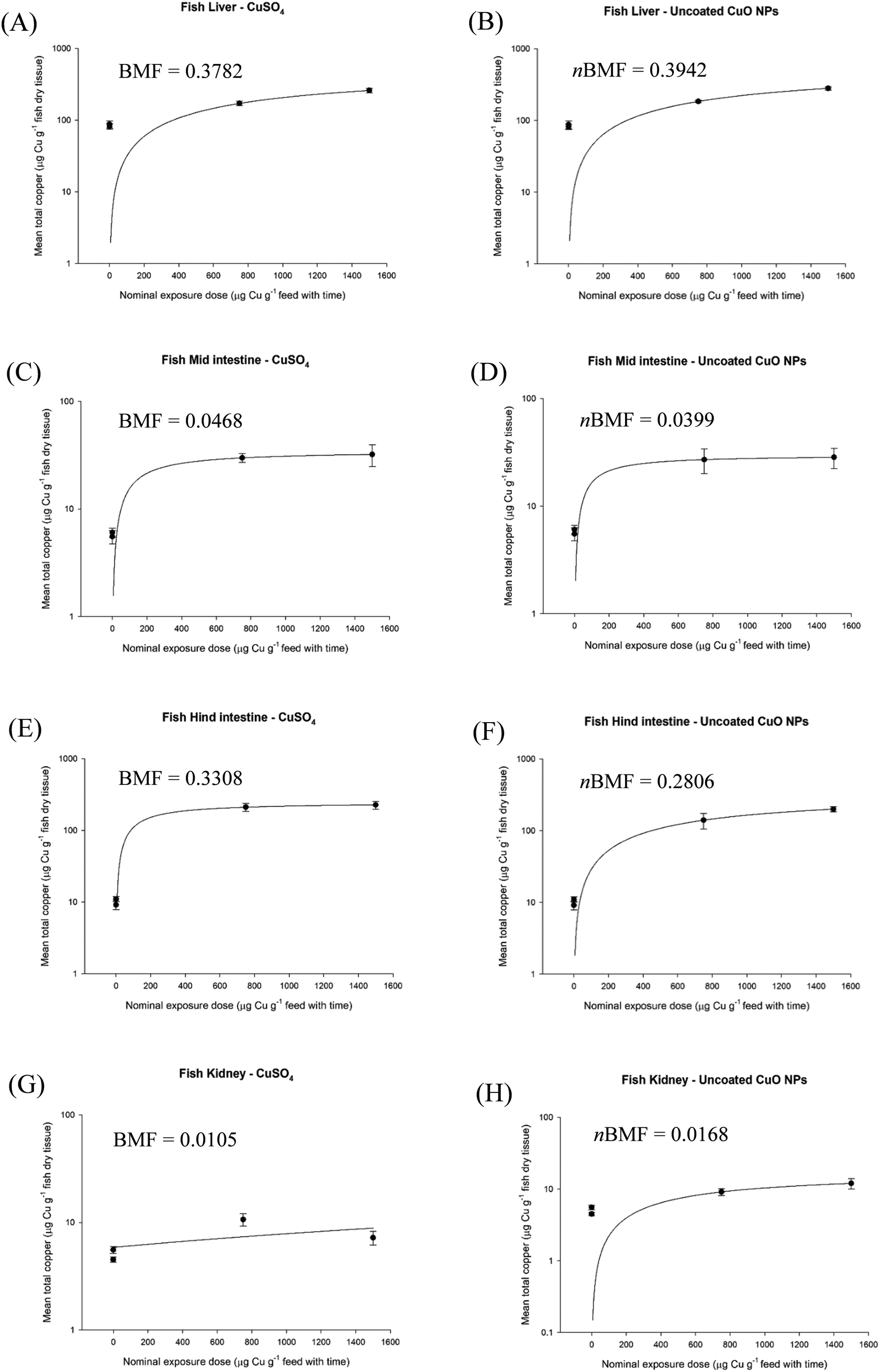Fig. 1 Nominal oral exposure dose of copper as CuSO₄ (left panels) and uncoated CuO NPs (right panels), plotted against measured total Cu concentration in rainbow trout (Oncorhynchus mykiss) liver (A and B), mid intestine (C and D), hind intestine (E and F) and kidney (G and H). Data are mean ± S.E.M, n = 9. Nominal oral dose is calculated from the nominal concentration in the food multiplied by exposure time. Animals were fed a fixed ration size of 2% body weight per day. Data are from Boyle et al.³⁶

Fig. 2 Nominal oral exposure dose of silver as AgNO₃, Ag NPs and Ag₂S NPs, plotted against measured total Ag concentration in rainbow trout (Oncorhynchus mykiss) liver (A–C), hind intestine (D–F) and kidney (G–I). Data are mean ± S.E.M, n = 4–6. Nominal feeding dose is calculated from the nominal concentration in the food multiplied by exposure time. Animals were fed a fixed ration size of 2% body weight per day. Data sourced from Clark et al.²

One might argue that the BMF value could be calculated for ‘newly acquired’ metal in the case of nutrients such as Cu, Zn, and Fe. However, the background of metal in the tissue can be difficult to distinguish from ‘newly acquired’ metal during the exposure as the turnover of both pools are as one in the homeostasis of total metal by the fish. This is especially a problem for Zn (ref. 39) and Cu.⁴⁰ Consequently, exposures to ZnO NPs up to 1000 mg kg⁻¹ for 39 days did not result in a persistent significantly elevated zinc concentration in the liver or blood,³ and 500 mg kg⁻¹ dietary ZnO NPs for six weeks did not increase internal organ concentrations above the natural zinc levels.³⁸ Such findings would result in a negligible BMF, or very difficult to calculate a BMF considering the background. In these situations, the use of an isotopically enriched MN may help to reveal any newly acquired metal over the existing background in the tissue.⁴¹ While this might reveal some mechanistic understanding, it is not routinely practical, or recommended here for contract research organisations (CROs) to do this when a nBMF based on total metal would be sufficient for risk assessment.

Here the BMF and nBMFs are derived from the total metal concentrations including data from the controls. The plots reach a plateau phase where the fitted line is apparently steady and the relevant BMF can be calculated from the tissue concentration in the animal at that point, and the measured concentration in the animal feed. Notice the plateau is not always completely flat, with a slight continuous rise (e.g., Fig. 1A). This is simply because the animal in vivo will never arrive at a perfect equilibrium, only a continuous steady-state. This was recognised during the development of the original bioaccumulation protocol with fish for organic chemicals, where very length exposures showed that a perfect equilibrium (i.e., net balance with zero loss or gain) was often not achieved.⁷ Copper saturation in the kidney was less clear for CuSO₄ (Fig. 1G), perhaps because this organ is known to produce large quantities of dilute urine in freshwater-adapted trout, but mainly because the organ simply did not accumulate additional Cu and so no saturation occurs.

Similar observations were made with CuO NPs, although the kidney tissue also showed a clearer plateau in net metal accumulation with the oral exposure dose (Fig. 1). Plots are also shown for the organs of trout in vivo following dietary exposure to AgNO₃, Ag NPs or Ag₂S NPs (Fig. 2). Notice, for all the Ag-containing substances the liver, hind intestine and kidney show a plateau in net metal accumulation, as expected for a non-essential toxic element that is not easily excreted.² The exception was the hind intestine for the Ag₂S NPs, where the organ total Ag concentrations remained low (i.e., no appreciable bioaccumulation, Fig. 2F). Nonetheless, for both Cu and Ag-containing MNs it is possible to show an apparent steady-state using a dietary method as in TG 305, so that an apparent nBMF is possible to determine.

The calculated nBMF values for fish whole body are shown in Table 2. Notice that all the apparent BMF or nBMF values for the whole body are below 0.1 or much less. In the case of dietary exposure to dissolved metals, and metal-containing MNs so far, the main target organs are the intestine (i.e., the route of entry) and the liver as a central compartment.^2,36,42 Consequently, the metal concentrations in these target organs are effectively diluted when they are homogenised or added to the rest of the body mass of non-target tissue (i.e., mainly skeletal muscle and bone), resulting in a low whole body burden measurement. The procedure for calculating the whole body burdens can include the gut, and carefully washed gut tissue was included in the whole body burdens used in the meta-analysis here. However, there is an argument for excluding the gut when there are concerns about residual food in the lumen. In such circumstances the whole body measurement may simply reflects dilution of the liver sample. Instead of whole body measurements, for metallic MNs we advocate using the trout liver directly to give a more realistic organ-specific bioaccumulation factor. The whole body burden approach was originally intended for lipophilic organic chemicals that might move by diffusion into multiple organs including the skeletal muscle. It remains unclear if this is a valid approach to organic MNs (e.g., pristine C₆₀, organic dendrimers, etc.,) and SWCNTs remain in the gut lumen without being appreciably absorbed by trout.⁴³ For MNs, organ-specific nBCFs, such as those from the liver may be the way forward.

Table 2 Biomagnification factors for dietary exposures to manufactured nanomaterials (nBMFs) calculated from data in the literature

Material	Primary particle size	Nominal exposure concentration	Whole body or organ concentration of metal (μg g^−1 dw)	BMF	Species	Comments	Authors
– Data not applicable to the test material.a Whole body values calculated from the sum of the individual organs plus the remaining carcass.b Whole body values measured from acid digests of the whole fish, unclear if/how the gut was included in the measurement.
AgNO3	–	100 mg kg^−1	3.925 ± 1.163^a	0.039	Oncorhynchus mykiss	Treatment of interest was compared to an unexposed control	Clark et al.^2
Ag NPs	50 nm	100 mg kg^−1	3.81 ± 0.796^a	0.038	Oncorhynchus mykiss	Treatment of interest was compared to an unexposed control and dissolved metal control	Clark et al.^2
Ag2S NPs	20 nm	100 mg kg^−1	0.321 ± 0.112^a	0.003	Oncorhynchus mykiss	Treatment of interest was compared to an unexposed control and dissolved metal control	Clark et al.^2
CuSO4	–	750 mg kg^−1	2.941 ± 0.722^a	0.004	Oncorhynchus mykiss	Treatment of interest was compared to an unexposed control	Boyle et al.^36
CuO NPs	18 nm	750 mg kg^−1	2.849 ± 0.848^a	0.004	Oncorhynchus mykiss	Treatment of interest was compared to an unexposed control and dissolved metal control	Boyle et al.^36
TiO2 NPs	21 nm	10 or 100 mg kg^−1	<0.4 in major organs	Negligible for organs	Oncorhynchus mykiss	Biomagnification factor cannot be calculated as the organ concentrations for total Ti were very low and at or around the background level in most organs including skeletal muscle. No bulk material control in the study because of natural Ti background in the animal feed	Ramsden et al.^1
ZnO NPs	25 nm	50 or 500 mg kg^−1	Background Zn 345–9 μg g^−1 as wet weight in major organs	Negligible for organs	Cyprinus carpio	No difference in total Zn concentration compared to the control following 6 weeks dietary exposure to either 50 or 500 mg ZnO per kg. Thus no appreciable Zn accumulation above the background. Skeletal muscle or carcass not reported so whole body concentration not possible to calculate	Chupani et al.^38
ZnO NPs	20–30 nm	300 or 1000 mg kg^−1	∼40 μg g^−1 as fresh weight or less in the liver	0.04 for the liver	Oncorhynchus mykiss	Only one time point showed slightly increased total Zn concentration in the liver of the treatments compared to the control following 11 days exposure to either 300 or 1000 mg ZnO per kg. Also no dissolved metal controls. Skeletal muscle or carcass not reported so whole body concentration not possible to calculate	Connolly et al.^3
TiO2 NPs	21 nm	0.1 mg L^−1	106.57 ± 14.89^b	0.024	Danio rerio	Fed on a diet of contaminated Daphnia for 2 weeks. Daphnia were exposed to 0.1 mg L^−1 of TiO2 for 24 h	Zhu et al.^62
TiO2 NPs	21 nm	1.0 mg L^−1	522.02 ± 12.94^b	0.009	Danio rerio	Fed on a diet of contaminated Daphnia for 2 weeks. Daphnia were exposed to 1.0 mg L^−1 of TiO2 for 24 h	Zhu et al.^62

---

For the nBMF calculations, the measured concentrations of metal in the fish feed were plotted against the measured metal concentrations in the individual organs of the fish for the last week (week 4) of the exposure (Fig. S1†). This provides data that can be used to calculate a measured nBMF that is more robust than estimating nBMFs from the nominal metal concentration in the feed. In all cases, the liver and the hind intestine had the highest total metal concentrations in vivo, and with lower concentrations in the mid intestine and the kidney for both Ag and Cu materials (Fig. S1†). A relatively low net silver accumulation was observed following exposure to dietary Ag₂S NPs in trout, typically between 1 and 10% of that accumulated in the other Ag treatments, because the Ag from Ag₂S NPs is not soluble or bioavailable.²⁹ Therefore, with negligible accumulation, any nBMF for Ag₂S NPs will be small.

With respect to particle metrics, the measured total metal concentration in the tissue at the end of the experiment can also be plotted against the physico-chemical properties of the materials. This has been done for primary particle size, hydrodynamic diameter in Milli-Q ultrapure water (18.2 MΩ, ELGA, UK), and the metal dissolution rate in the same ultrapure water (Fig. 3A–C), for the test materials CuO NPs, Ag NPs, Ag₂S NPs. However, for regulatory use, the main interest is to plot these particle metrics against the measured nBMFs for rainbow trout organs in vivo. Data are shown for liver, mid intestine, hind intestine and kidney, respectively (Fig. 3D–F), with the equations for the fitted lines (Table S1†). A significant positive correlation (Spearman's correlation, p < 0.01) was observed for metal dissolution rate, when fitted against the measured nBMFs in the liver, mid-intestine, hind-intestine and kidney, respectively, in trout (Fig. 3F). For particle size (Fig. 3D) and hydrodynamic diameter (Fig. 3E), no statistically significant correlations (Spearman's correlation, p > 0.01) resulted with the fish nBMFs. Regardless, for all particle metrics investigated, the measured nBMF for the liver showed the steepest correlations and therefore the most promise for regulatory use (Fig. 3D–F). However, the data set is small, and more data values for measured nBMFs from in vivo, using studies with trout in TG 305 are needed to expand the analysis for different shapes, sizes, chemical compositions and a wider variety of coatings. Nonetheless, the steps in the data processing are demonstrated and the approach is promising. Notice that the r² values for primary particle size and metal dissolution rate in the liver, can account for most of the variation in the data (Fig. 3). Multiple regression was then used to determine if a prediction equation for nBMF could be defined from all the particle metrics. The primary particle size, hydrodynamic diameter and dissolution rate were first used as independent variables, and the fish organ nBMF as the dependant variable. In all organs, the hydrodynamic diameter was removed in subsequent reiterations because of collinearity, leaving the primary particle size and dissolution rate as the main predictors of the data. For example, these two variables predicted 83.0, 67.6, 82.0 and 61.4% of the variance of the data in the liver, mid intestine, hind intestine and kidney (all p < 0.001), respectively (Table S2†). A regression prediction equation was fit to the liver nBMF data using eqn (1);

y = −0.639 + (0.0206 × a) + (28.066 × b) (1)

where y = liver biomagnification factor, a = particle size and b = dissolution rate.

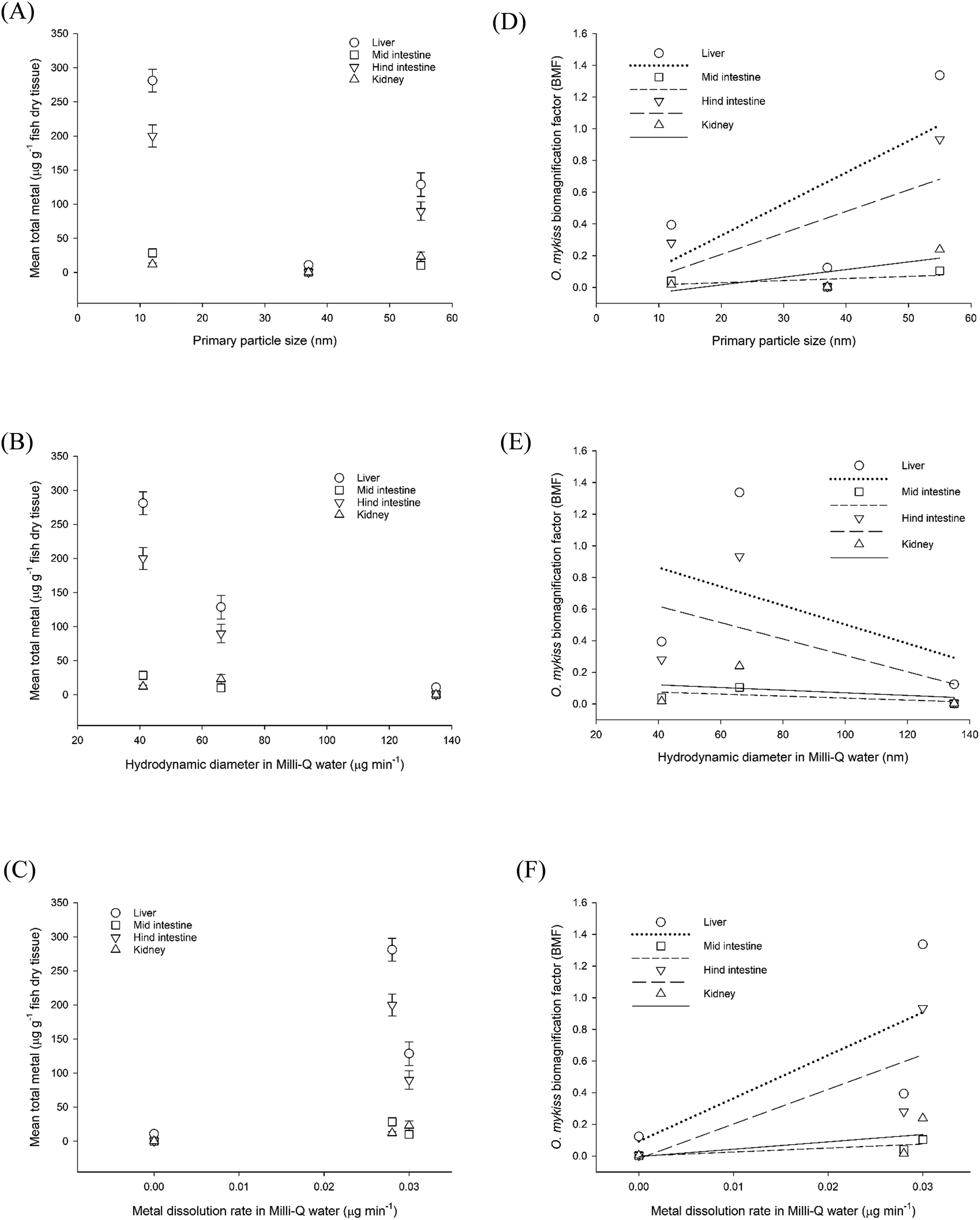Fig. 3 Nanomaterial physico-chemical properties plotted against total organ metal concentration (left panels) or organ bioamagnification factors (BMFs) (right panels). Properties of primary particle size (A and D), hydrodynamic diameter (B and E) or metal dissolution (C and F) were considered against the liver, mid intestine, hind intestine or kidney in rainbow trout (Oncorhynchus mykiss). Data are mean ± S.E.M, n = 4–6. Organ total metal concentration measured after 4 weeks exposure to either uncoated CuO NPs, Ag₂S NPs or Ag NPs. The r² values for liver, mid intestine, hind intestine and kidney are 0.45, 0.30, 0.38 and 0.62 in plot (D), 0.21, 0.35, 0.28 and 0.09 in plot (E) and 0.51, 0.67, 0.59 and 0.35 in plot (F), respectively. Equations for the curve fits are in Table S1.† Silver data from Clark et al.² and copper data from Boyle et al.³⁶

Data mining for nBMF values in fish to avoid new in vivo testing (tier 2)

One approach to minimise the use of the in vivo fish bioaccumulation test is to obtain nBMF values from the existing literature, rather conducting new tests with TG 305. Some nBMF values derived from the scientific literature are shown (Table 2). Data mining could expand the available data sets on nBMF values available for a REACH risk assessment. Any data mining from the scientific literature should be systematic, and with set quality criteria on the scientific papers used, in order to be reliable for a REACH risk assessment. The Klimisch score for reliability has already been applied to the dossiers on the toxicity of MNs at the OECD.⁴⁴ It remains to be agreed at the OECD on exactly what ‘extra’ criteria should be included for the scoring of studies of MNs found in the literature, so that they might be used in a REACH risk assessment. The approach in the current study was in the spirit of the Klimisch score, but with additional criteria for particle characterisation.

The criteria were: (i) appropriate particle characterisation through measurements of primary particle size and/or hydrodynamic diameter in ultrapure water; (ii) measured metal concentrations in the test media that confirmed a consistent exposure and within 80% of the nominal concentrations; (iii) measured metal concentrations in the test organism were reported, and were detectable given the variation of background concentrations of metals in the control animals; (iv) evidence of quality assurance in the procedures for metal analysis, such as procedural blanks, spike recoveries, analysis of certified reference materials and internal standards to check for instrument drift over the course of the analysis; (v) the experimental design was replicated, at least n = 3 tanks per treatment; and (vi) the experimental design had unexposed controls, and metal salt controls or bulk material controls as appropriate for a MN study design.

This very stringent approach to criteria for data mining was immediately problematic, with very few studies meeting all the criteria, and there are some nano-specific issues that can prevent the criteria being applied to a dietary exposure. For example, Ti is ubiquitous in biota and inevitably becomes incorporated into fish feeds made from fishmeal, and other similar ingredients. Indeed, traditional TiO₂ powder is used as an inert marker in feed manufacture and is widely found in fish foods (see the dietary study of Ramsden et al.¹). The problem is the natural Ti in commercial animal feed is impossible to remove without compromising the nutritional value of the feed. In such situations, a bulk material control is somewhat redundant as the ‘unexposed’ control already contains TiO₂,¹ so the criteria of insisting on bulk material control is not useful in that circumstance. Also, with no strong evidence of the accumulation of ‘new’ Ti in the tissues,¹ any calculated nBMF for TiO₂ would be negligible (Table 2). Similarly, removing naturally occurring iron from animal feed is very difficult with respect to ensuring the overall nutritional value of the food,⁴⁵ and it may be particulate. Quality assurance criteria are also problematic, and while spike recovery tests may be conducted with tissues, there are currently no certified standard reference tissues for fish for MNs. Nonetheless, we recommend using nBMFs from the literature, especially organ-specific values, and to apply these in risk assessment with caution, but also in the spirit of avoiding further in vivo testing. Any caveats attached to a nBMF value could be reported to make the limitations of the specific study clear.

‘In vitro’ fish: digestibility assay and gut sac experiments to predict bioaccumulation potential (tier 3)

There are two parts proposed for this tier, the in chemico digestibility assay and the ex vivo gut sac technique.⁶ These assays are intended as an ethical justification to move to in vivo fish bioaccumulation experiments; only if both assays show positive results should the TG 305 begin (Fig. 4). This step should therefore reduce the number of fish used for in vivo testing, by only going forward to the final tier with materials of concern. The digestibility assay is a sequential simulation of some of the key events in gut lumen chemistry that might lead to the MN in food becoming bioaccessible to the gut epithelium, and therefore ultimately bioavailable for uptake by the fish. Our approach is similar in principle to the BARGE sequential extraction applied to determine bioaccessibility of MNs in soil,²⁶ but derived for a simplified digestion process in fish gut lumen.⁶ Sequential extractions were performed in 0.9% NaCl, saline plus 10 mmol L⁻¹ ethylenediaminetetraacetic acid (EDTA), and then in saline plus 0.1 M HCl, with an optional step using a digestive enzyme mix, and finally a strong acid digestion in aqua regia to determine the remaining metal dissolution.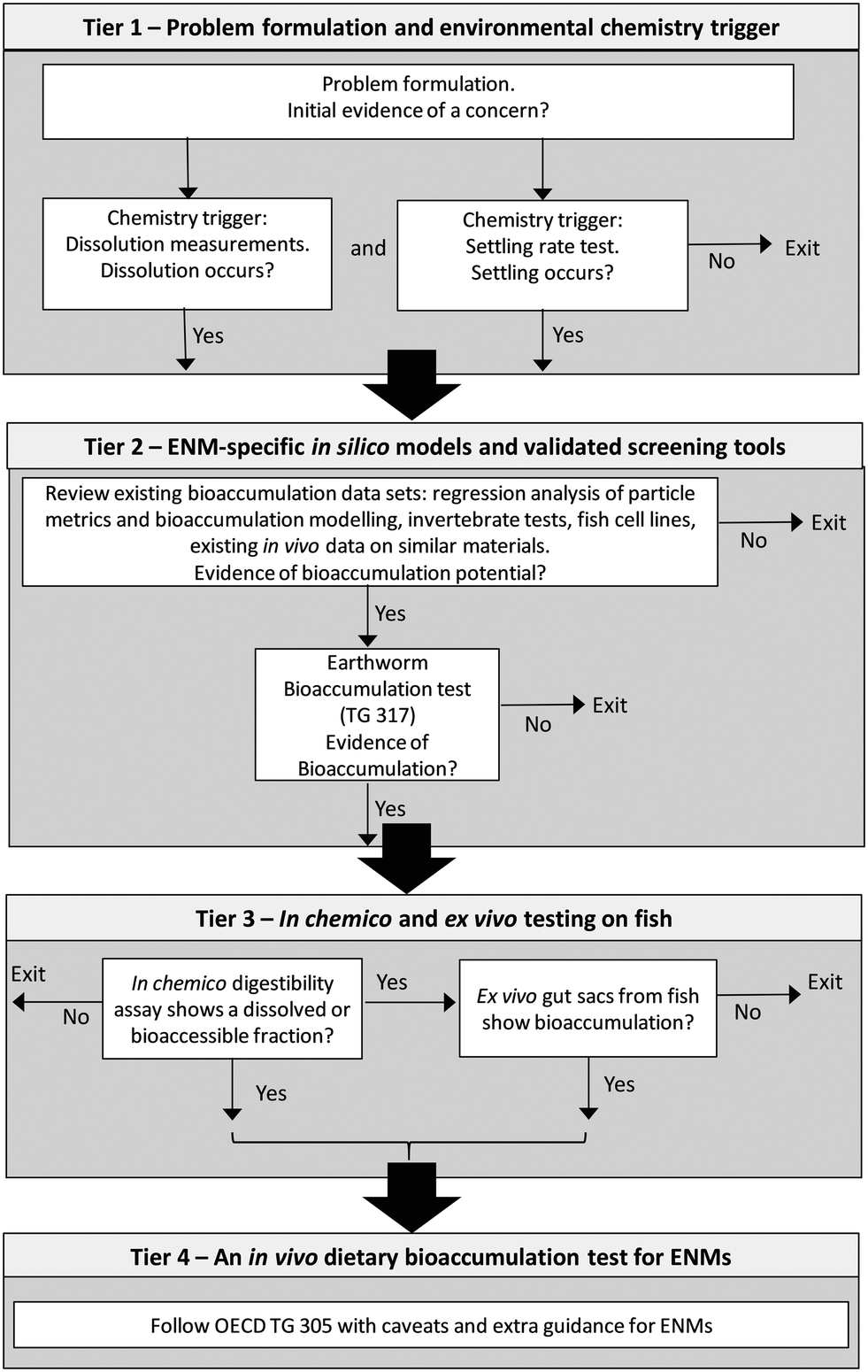

Fig. 4 A proposed decision tree for working through the bioaccumulation testing strategy for manufactured nanomaterials (MNs), with scientific exit points in the early tiers. ‘Exit’ indicates leaving the strategy at the point in the tier indicated without proceeding to the next step or tier.

The second half of this tier is the gut sac method (Fig. 4). This approach uses the intact epithelium, but with anatomical regions of the gastrointestinal tract isolated from the fish (i.e., ex vivo), with the gut lumen filled with the MN of interest in a physiologically relevant gut saline and incubated for 4 hours. At the end of the incubation, any excess media is rinsed off the tissue and the gut mucosa separated from the underling muscularis. The compartments i.e., luminal solution, mucosa, muscularis, and serosal solution (blood side) are then measured for the substance of interest to determine any accumulation in the tissue or transepithelial uptake across the gut. The gut sac approach has a long history and was originally used to measure the physiological transport of solutes across the gut of animals.⁴⁶ It has also been applied to dissolved metal uptake by fish e.g., Cu,²⁷ Hg,⁴⁷ the absorption of organic chemicals such as benzo[a]pyrene,⁴⁸ and to MNs in fish e.g., TiO₂;²⁸ Ag NPs²⁹ and CuO NPs.³⁴

Does the in chemico digestibility assay predict in vivo bioaccumulation?

The in chemico digestibility assay should inform on any bioaccessible fraction of the test substance in the gut lumen that is derived by the simulated ‘digestion’ of the food. The assumption is that any bioaccessible fraction from the MNs in the food pellets (e.g., dissolved metal, or free particles released from the food matrix) is also bioavailable. This would therefore lead to bioaccumulation, or at least some measurable uptake into the internal organs of the animal, if the bioaccessible fraction occurred in vivo. For example, the digestibility assay showed that a few percent of the ingested dose is bioaccessible from trout feed containing AgNO₃ or Ag NPs, but less than 1% as total Ag from Ag₂S NPs.⁶ For the same MNs, the in vivo study with trout confirmed this ranking of the materials, with the dietary bioaccumulation potential being in the order: AgNO₃ = Ag NPs > Ag₂S NPs. The Ag₂S showed very low accumulation in the organs of trout in vivo, in keeping with a digestibility of <1%.

Notably for metal and metal oxide MNs, the 0.1 M HCl digestion step (simulating the low pH of the stomach in trout) reveals the most bioaccessible fraction, as is also the case in the BARGE method with CuO NPs.²⁶ Dissolution studies also show that some metal-containing MNs dissolve faster at acidic pH, e.g., CuO NPs,^34,49 and the resulting total dissolved metal may contain free metal ions depending on the speciation chemistry of the media. So for metal MNs, it may be possible to simplify the in chemico assay further to just the ‘acid digestion’ step in the stomach. When 100 mg kg⁻¹ of total Ag (as AgNO₃, Ag NPs or Ag₂S NPs) are incorporated into the fish diet and undergo exposure to the stomach compartment simulated digestion (0.1 M HCl at pH 2) for 4 hours, the total metal released is 27.1, 44.9 and 4.1 μg Ag per g for the different Ag materials, respectively. For Cu diets containing 750 mg kg⁻¹ of total Cu (as CuSO₄ or CuO NPs), the release of metal was 202.6 and 246.3 μg Cu per g for the Cu materials, respectively. When the same diets were fed to fish for 4 weeks, the fish liver concentrations were 128.6, 121.8 and 11.0 μg Ag per g exposed to either AgNO₃, Ag NPs or Ag₂S NPs, respectively,² and 259.3 and 281.3 μg Cu per g exposed to CuSO₄ or CuO NPs, respectively.³⁶ These values of ‘total dissolved metal’ released should be interpreted as a total measured by ICP-OES or ICP-MS, not the free metal ion concentration alone, but the sum of the dissolved metal species plus any incidental metal particulate released into the media. Correlation analysis of these data show a significant relationship between the total metal released in the stomach compartment of the digestibility assay and the total metal concentration in the liver of the relevant in vivo dietary exposure using trout (Pearson's correlation coefficient, 0.946, p = 0.02, r² = 0.894). Thus illustrating the digestibility assay as a very good indicator of the accumulation in the liver in vivo.

It is also possible to run the digestibility assay with the food pellets inside dialysis tubing to reveal any dissolved versus particulate fractions released from the food. Clark et al.² placed the diet in dialysis tubing and by sampling the external media identified the dissolved metal fraction for the Ag-containing MNs. This approach demonstrated that AgNO₃ and Ag NPs in the food pellets released equal amounts of dissolved Ag, but there was no dissolved Ag release from the Ag₂S NP treatment; indicating dissolution of the former two treatments and a potential particle exposure from the latter.² The digestibility assay is a rapid, sensitive, reproducible, and cheap test, and from a practical viewpoint, lends itself for regulatory use for metallic MNs. Some further consensus building and inter-laboratory testing would be needed to validate this as a standard method for metallic MNs, and to define the thresholds for a bioaccessible fraction of concern that would trigger moving to the final tier in the testing strategy.

The digestibility assay to simulate aspects of the fish gut lumen has not yet been applied to organic MNs (e.g., pristine C₆₀, SWNCNTs, dendrimers, etc.), but in principle, provided any steps involving water or dilute acid extractions, and so on, did not degrade the MN of interest, then the methodology would work. The technical barrier for organic MNs is the quantitative detection of the MNs in the tissue in the first place, so any bioavailable fraction can be calculated; and also refinements to detect them in the potentially complex matrix extracted. Similarly, any organic coatings on particles should preferably not appreciably degrade during the extractions. However, these problems are fundamentally no different to assessing the digestibility of the organic substances that are nutrients in animal feed (lipids, carbohydrates, fat-soluble vitamins, etc.) and the approach has had utility in fish nutrition for many years.²³

Is the ex vivo gut sac method predictive of in vivo bioaccumulation from nanomaterial exposures?

In the proposed tiered approach (Fig. 4), the gut sac method is a second aspect of in vitro fish work in tier 3,⁶ with the notion that any accumulation observed in the gut sacs would infer an in vivo bioaccumulation potential. This is also an exit point from the testing strategy. If tier 3 shows no effects, then arguably one should not proceed to the dietary in vivo test (TG 305) in tier 4. The gut sac method shows that the intestines accumulate the most metal for MN exposures, e.g., mid intestine,²⁹ as expected from the known absorptive functions of the intestines of vertebrate animals.

However, for the purposes of predicting effects in vivo (tier 4), it is also crucial to know what is the best tissue compartment from the gut sacs for those predictions. In oral toxicology, the focus is often on the gut mucosa itself, since this is the tissue layer involved in the active uptake of substances from the gut lumen. One might also argue that measuring the presence of the test substance in the mucosa would confirm it is bioavailable, as well as being a prerequisite step before bioaccumulation by the organism. However, test substances can be lost with the turnover and sloughing of the mucous epithelium in vivo, or the test substance might become ‘trapped’ in lipid bilayers of the gut epithelium and not pass to the blood supply, e.g., organic chemicals with a high log K_ow.⁵⁰ Export of solutes or MNs from the epithelial cells via the serosal (basement) membrane to the blood is also the rate-limiting step in absorption.⁵¹ Thus, the presence of a substance in the mucosa does not necessarily infer it will bioaccumulate in the internal organs in vivo. Alternatively, one might use the underlying muscularis from the gut sacs for predictions (i.e., the remaining gut tissue minus the mucosa). The advantage here is that the muscularis portion is on the serosal (blood) side of the preparation, and so any MN, or total metal from MNs, present would represent an in vivo bioaccumulation risk. The presence of the test substance in the muscularis portion of the gut sac within a 4 hour incubation is not usually interpreted as uptake by the smooth muscle itself; but rather that the test substance is most likely in the vasculature, lymphatics, and extracellular space going through that layer. As such, this would be rapidly exchangeable with the rest of the systemic blood supply in vivo.

The data from gut sac experiments with Ag materials²⁹ and CuO MNs³⁴ were plotted against the in vivo data from trout (Fig. 5 for the mucosa; Fig. S2† for the muscularis). The total metal concentration in the mucosa of the gut sac experiment plotted against that of the liver from in vivo experiment for dissolved Ag or Cu salts (Fig. 5A and D) showed a significant relationship (CuSO₄, Spearman's correlation coefficient, 1.000; AgNO₃ Pearson's correlation coefficient, 0.957; both tests, p < 0.01). The same positive relationship was also observed in the CuO NPs, Ag NPs and Ag₂S NPs treatments (Fig. 5B, C and E; Spearman's or Pearson's correlation coefficients were 0.874 (p < 0.01), 1.000 (p < 0.01) and 0.956 (p = 0.02), respectively). These are good correlations, illustrating that the total metal concentration from an MN exposure in the mucosa is predictive of the accumulation in the liver of fish in vivo, and that the mucosa could be used as a surrogate indicator of the bioaccumulation potential. In terms of regulatory acceptance, the gut mucosa as the initial point of uptake from a dietary exposure is widely understood.

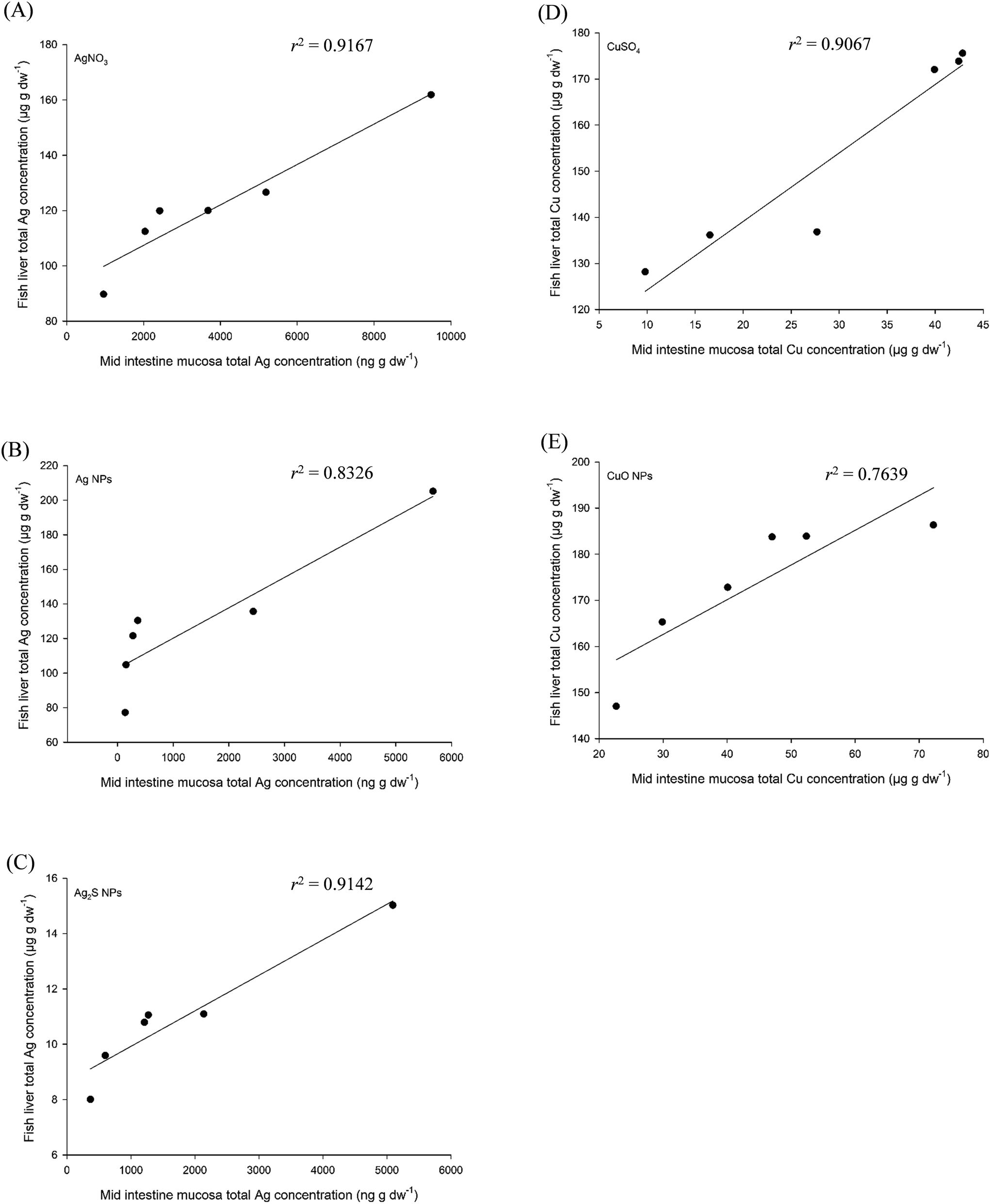Fig. 5 Correlations between tier 3 (ex vivo exposure with gut sacs, mid intestine mucosa) and tier 4 (in vivo exposure, liver concentrations) of the testing strategy. The materials used are silver (left panels) or copper (right panels) based. The data were ranked and then correlated. The equation of the lines are (A) y = 0.0073x + 92.812, (B) y = 0.0176x + 102.6, (C) y = 0.0013x + 8.6417, (D) y = 1.4855x + 109.41 and (E) y = 0.7562x + 140.05. Copper data sourced from Boyle et al.³⁴ Silver data sourced from Clark et al.^2,29

Alternatively, the muscularis could be used for the correlations. When the total metal concentration in the muscularis from the ex vivo gut sac experiment is plotted against the liver concentration in vivo, there is a positive correlation for all Ag treatments (Fig. S2A–C†). The same is true for the CuSO₄ treatment, but with the CuO NPs the relationship is not linear, although all show some correlations with in vivo (Fig. S2D and E†). The reasons for the non-linear aspect of plot for the CuO NP exposure (Fig. S2E†) is not clear, but might relate to trout liver being able to store biogenic Cu particles.⁵² Regardless, while the correlations using the muscularis are mostly acceptable (i.e., mostly exceeding an r² of 0.73, Fig. S2†), the correlations for the mucosa (Fig. 5) are slightly better. Thus, it is possible to use the mucosa from gut sac data as a screening tool, and this would be in keeping with scientific tradition to focus on the epithelial cells. However, for certainty of logic in regulatory decision making, the muscularis offers the unequivocal advantage of demonstrating internal uptake because it represents the serosal side of the gut. Clearly, both the mucosa and the muscularis of the gut sacs may be a useful predictive tool. Similar to the digestibility assay above, the dearth of detection methods for organic MNs in tissues would need to be overcome to use the technique more widely for all MNs, although radiolabelled MNs (e.g., carbon-14) could be detected in biological matrices using existing methods, such as liquid scintillation of freeze-dried tissues.⁵³

Can a biomagnification factor be derived from gut sac experiments?

The gut sacs studies are intended to inform on whether or not to proceed to the in vivo fish test, TG 305. However, it is possible to calculate BMF values for different anatomical regions of the gut from the gut sac studies. For instance, the AgNO₃, Ag NPs or Ag₂S NPs BMF or nBMF values for the mid intestine were 0.231 ± 0.110, 0.072 ± 0.101 and 1.027 ± 1.096, respectively. Similarly, for the hind intestine with AgNO₃, Ag NPs or Ag₂S NPs, the BMFs or nBMF as appropriate were 0.145 ± 0.050, 0.067 ± 0.054 and 0.231 ± 0.168, respectively. These can then be compared to the derived in vivo BMF. From in vivo dietary exposures, the BMFs or nBMFs as appropriate for the mid intestine were 0.009 ± 0.001, 0.009 ± 0.001 and 0.0005 ± 0.0001 for the AgNO₃, Ag NPs and Ag₂S NPs treatments respectively. The silver treatment BMFs or nBMFs from the two experiments were plotted against each other (data not shown). Both the mid intestine and hind intestine produced strongly negative correlations, with r² values of 0.9821 and 0.7943, respectively (Spearman rank order correlation coefficients of −1). The equation of the line for the mid and hind intestines are y = −0.0095x + 0.0106 and y = −0.0531x + 0.0142, respectively. While these initial correlations are good, they were not always statistically significant due to the limited size of the data set, and more data from other materials may strengthen any prediction equations or derived correlations.

In vivo dietary exposure using fish, TG 305 (tier 4)

The fish bioaccumulation test was originally devised for exposures to organic chemicals via the water, and where steady-state was achieved between the water and tissue concentrations of the test substance, a BCF could be calculated.⁷ However, it was recognised that maintaining an aqueous exposure for chemicals that are ‘difficult to handle’ in water is problematic for a regulatory test, and so the dietary exposure method was incorporated into the current version of TG 305,⁵ and with additional guidance on how to do the calculations for a dietary exposure.⁵⁴ Given the propensity of MNs to agglomerate, aggregate and settle in water, the dietary exposure method has been recommended to maintain the exposure for MNs.⁶

For the data sets in the present study, it was possible to show that the organ total metal concentration from the relevant MN exposure was at or approaching an apparent steady-state (e.g., Fig. 1 and 2) to enable a nBMF estimate for key target organs, and/or the whole body (Table 2). It is recognised that conducting in vivo dietary exposures with fish is a logistical challenge, and pragmatically the exposure phase of OECD TG 305 typically lasts up to 14 days and with data from only one oral exposure concentration at a fixed ration.⁵ Similarly, research studies may restrict the number of concentrations and time points because of the additional controls and logistics needed for MN experiments.¹⁵ For example, the data sets here on CuO NPs with two time points plus the time-zero control,³⁶ although there can be more time points when understanding the kinetics of MN uptake is the main objective (e.g., five time points for Ag materials used here,²). However, this is not a barrier to determining the bioaccumulation potential of MNs.

Our approach is to maximise the utility of in vivo data in the meta-analysis by using dose, this enables the plots to be made with one treatment/group of animals (i.e., one exposure concentration) that is followed over time to obtain dose. This would use fewer fish than repeating the measurements at multiple exposure concentrations (multiple groups of fish) over time. Our approach is in keeping with animal welfare considerations to minimise the use of animals. Arguably, whether the exposure is followed as a function of fixed concentration over varied time, or vice versa, is somewhat academic. It is the oral dose at a fixed 2% ration (i.e., dietary concentration × time eating it) plotted on the x-axis against the measured concentration in the fish organs that can best reveal the apparent (dynamic) steady-state needed for nBMF calculations (Fig. 1 and 2). The guidance for metals under REACH also recognises the problem of using exposure concentration alone to calculate BMFs,¹³ and the guidance on metals risk assessment from the US EPA highlights the importance of target-organ specific responses,¹⁴ as we have done here. Applying precaution to the analysis, the BMFs or nBMFs as appropriate for the solute or MN respectively, were ultimately calculated for the organ or whole body concentration at the last time point of the exposure in the studies (i.e., week 4) and the concentration in the feed at a fixed 2% ration. The whole body nBMFs for metal-containing MN exposures to fish are, so far, very small; and perhaps misleading because of the diluting effect of the whole body measure on target organ concentrations discussed earlier. For example, nBMFs calculated here for fish whole body of 0.038 and 0.004 for Ag and CuO NPs, respectively (Table 2), and for reasons of dilution in the whole body the BMFs for the metal salts are similarly low. The guidance for TG 305 offers mathematical techniques (intended for solutes not MNs), for correcting whole body data for growth dilution, dietary absorption efficiency when the ration changes, and/or to normalise for lipid content in the case of organic chemicals.⁵⁴ However, we recommend calculating BMFs or nBMFs from the target-organ specific concentration of total metal, especially for the liver, which showed the highest values for the nBMF (Fig. 1 and 2). Connolly et al.³ also attempted a nBMF calculation for the liver of trout exposed to ZnO NPs via the diet.

The need for dissolved metal and/or bulk (micron scale) material controls has been also highlighted for nanoecotoxicology in order to infer whether any effects are due to particles/particle size, or simply a chemical effect of the substance.¹⁵ Such information is important from a risk assessment perspective. For instance, to know if any new MN is more, or less hazardous, than any existing substance of the same chemical composition. However, the 3Rs should be implemented in the bioaccumulation testing strategy at every opportunity. One might argue that the metal salt controls are not needed since BMFs for these substances are already known. Similarly, the requirement for metal salt controls could be relaxed in primary research for the same reasons. On the other hand, there are many variables that could influence the nBMF value obtained from a primary research study (i.e., not a standardised test). These include the precise water chemistry, temperature, ration size, and even the stocking density of the fish and their ability to form social hierarchies that influence the feeding behaviour and ingested dose of individual animals in the exposure.⁵⁵ Therefore, within-study metal salt controls can at least remove those sources of variation from the data analysis of individual experiments.

Finally, one should be clear on what any apparent nBMF has measured in any in vivo bioaccumulation test with fish. In the majority of studies so far, there is no measurement of particle number concentration or particle sizes inside the tissues, except for the spICP-MS study of silver.⁴ Therefore, it is not a BMF for the nano form per se. For environmental risk assessment, one should remember that any nBMFs are calculated on the basis of total metal concentration in the tissue for a dietary MN exposure. Notably, Clark et al.²⁹ found that exposure to AgNO₃ also resulted in the appearance of Ag-containing particles in the liver; perhaps due to AgCl particle formation in the gut lumen and/or biogenic particle formation in the tissue. Similar observations have been made in earthworms with Ag-containing particles being formed in animals exposed to AgNO₃.⁵⁶ If such processes are occurring in tissues, it may be difficult to determine a nBMF on the basis of particle number concentration, and this would rely on a dynamic steady-state between the exposure, biogenic particle formation and biodegradation. An agreed standardised protocol for spICP-MS, and how to use that in TG 305, or any other OECD test for bioaccumulation, is some way off. At the present time it is recommended that nBMF can be calculated on the basis of total metal concentration in the organs. The application of TG 305 to organic MNs such as C₆₀ or carbon nanotubes is discussed elsewhere,⁶ but again, the dearth of techniques for detecting such intact MNs in tissues is limiting the application of the TG 305 to radiolabelled organic MNs at this time.

Decision tree and exit points from the testing strategy

Fig. 4 shows a possible scheme needed in order to guide the user through the tiers in the testing strategy and to offer clear guidance on implementation. This scheme is modified from Handy et al.,⁶ with additional information to show the exit points from the strategy. Details of how to use the chemical triggers in tier 1 to move to tier 2 are discussed elsewhere.²² Briefly, the scheme starts with the problem formulation and the initial evidence of concern, as would usually be the case for any hazard assessment. For example, the MN might be designed to be persistent, or have agricultural applications that make exposure via the food chain more likely. The chemistry triggers in tier 1 are dissolution and particle settling, both triggers need to be positive to move to the next tier. For example, if dissolution was negligible (e.g., no ‘free metal ion’ bioaccumulation concern) and the MN showed no evidence of particle settling to contaminate the base of the food web, then the bioaccumulation concerns would be low and one could exit the strategy.²² Albeit with some caveats about marine fishes that could drink seawater containing any MNs that remained in the water column, and/or exceptions for waterborne uptake through the gills.²² In the present meta-analysis, we also illustrated how prediction equations for nBMFs in fish might be calculated from data on particle properties (Fig. 3), and in the absence of a single metric to completely describe bioaccumulation, we report a ‘best’ prediction equation derived from a combination of these MN metrics. The predictions here are based on a few MNs with different chemistries, coatings and sizes, and the scientific community will need to agree when a prediction equation is robust enough to apply to regulatory decision making for MNs. Nonetheless, if prediction equations could be agreed, then it might be possible to use them in the problem formulation step early on in tier 1. For example, if the predictions from particle metrics gave a nBMF > 1 then one might proceed directly to tier 2. The prediction equations might also find utility in safe-by-design manufacturing, where the physico-chemical properties associated with the bioaccumulation potential might be adjusted to a combination where bioaccumulation would be less likely.

In tier 3, it is proposed that the in chemico digestibility assay is conducted first. Again, some consensus building by the scientific community is needed to agree on the threshold values for a positive outcome in this test. However, for dissolved metals, one might consider that in vivo, only a few percent of the ingested dose is enough to initiate bioaccumulation in the long term (see review on dietary metals in fish⁴²), and so the threshold for the outcome of the digestibility assay could be very low. For example, around 1% of the dose released as dissolved metal for MNs containing non-essential toxic metals such as Ag, Cd, Pb or Hg. The relationship between digestibility of food in the simulated gut lumen of fish and the release of intact MNs that might then be bioavailable for uptake at the gut mucosa is less clear, but for example the thresholds for relatively insoluble and inert MNs in the gut such as TiO₂ (ref. 1) might be set with a higher threshold. Further work to collect data with digestibility assay with a range of MNs and compared to in vivo is needed to help define where the threshold values should be and if those thresholds would need to be substance-specific rather than for groups of chemically similar MNs.

For nutritionally essential metals such as Zn or Cu, these tend not to bioaccumulate because their homeostasis is controlled by metal ion transporters, but even these systems can be overloaded, and so thresholds for these metals could be set around the known nutritional requirements of fish.⁵⁷ The same threshold could be used for the nano forms of essential metals in the first instance, until more data sets were available to refine any agreed thresholds for MNs. The situation for organic chemicals being released from MNs during the digestibility assay could follow a similar thinking to that above. For example, organic chemicals are taken up across the gut according to their lipid solubility (log K_ow measurement) which of course also depends on the polarity of the substance (dipole moment, or even ionised to make it soluble in water). So, existing computational models could be used that consider lipid solubility, the membrane resistance/permeability of the gut, rate constants for metabolism of the substance, etc.,^58,59 to help understand what the threshold should be in the digestibility assay. Or the quantitative structure activity relationships (QSAR) that exists between log K_ow values for the organic chemicals and their steady-state BMF in fish.⁶⁰ If the organic MN becomes bioaccessible in its intact form, then a threshold would need to be decided, but given that many organic chemicals can be metabolised in vivo, these thresholds for intact organic MNs might not be as low as those for non-essential metals.

If the in chemico digestibility assay result is negative, then one can exit the testing strategy. If the result is positive, then gut sac studies should be done on the mid and hind intestine of the fish, and preferably for the same species as would be used in any in vivo test. The gut sac will enable the calculation of a nBMF for the intestine. To harmonise with existing use of BMF values, the general guidance by the European Chemicals Agency⁶¹ could be applied, but with some modifications for MNs. These modifications for MNs should be agreed by consensus, but for example, if the nBMF is <1, and the in chemico digestibility assay shows a negative result or very low digestibility, then it would be hard to ethically justify moving to the in vivo test in tier 4, and so one would exit the strategy in tier 3. It would also be hard to ethically justify moving to tier 4 if the threat from the MN was mainly arising from dissolution of dissolved metals. For example, if the in chemico digestibility assay showed the bioaccessible fraction is only from a dissolved metal with none of the intact MN remaining, and the MN dissolves in saline such that gut sacs would be exposed to only dissolved metal, then one might argue that the existing dissolved metal data on fish should be used, rather than conducting a new in vivo test. The final tier 4 should be conducted according to TG 305 with the caveats for MNs, as previously described.⁶ Crucially, the multiple tiers in the scheme will be conservative in that evidence could be sought from several different tests or assays, thus minimising the risk of false negatives or positives. The scheme does not, however, represent an ‘extra’ burden of work or ‘additional’ cost for a manufacturer of nanomaterials seeking to prepare a dossier of environmental safety data for product registration, or for a contract research laboratory conducting regulatory tests. Much of the information in tier 1 on the physico-chemical properties of the MN, such as primary size and the behaviour of dispersions, is likely to be integral to the product description, how it is supplied to customers (e.g., dispersed in liquid), and/or part of the safe-by-design innovation. Tier 2 will use existing information in the literature and an earthworm bioaccumulation test, which is already a routine part of environmental hazard assessment. The rapid in vitro tests in tier 3 may enable a decision to avoid the in vivo fish bioaccumulation test entirely, thus avoiding those latter costs.

Conclusions

The data analysis here shows that dietary exposures to metal-containing MNs in trout, conducted according to the principles in TG 305, can show an apparent steady-state for total metal concentrations in the tissues compared to the food. Thus, pragmatically, it is possible to derive a nBMF for exposure to MNs and total metal concentrations in the organs of fish. Here, we have shown a digestibility assay that simulates the gut lumen of fish is simple, rapid and a useful tool to identify if a bioaccessible fraction is present that might lead to a bioaccumulation concern. The ex vivo gut sac also correlates with in vivo. Where both these methods show a negative result, it implies a negligible bioaccumulation concern, and therefore moving to in vivo testing on fish would not be ethically justified. These tools are precautionary with safety (i.e., no false negatives) and could find utility in a tier approach to testing that minimises the use of TG 305.

Author contributions

DB, NC, and TB conducted the original experiments that provided the data set used here, from the EU projects acknowledged below. JV and NC conducted the meta-analysis with input from RDH, CG, FN, CS, NvB and VW. Manuscript preparation and writing of the drafts was led by RDH, with JV and NC preparing the data illustrations and statistics. All the co-authors read subsequent drafts.

Conflicts of interest

The authors do not declare any conflicts of interest.

Acknowledgements

This work was supported by grants from Defra UK awarded to RDH (project number 27891; also Project to support a scoping review on the bioaccumulation of nanomaterials), and from the European Union's Horizon 2020 research and innovation programme: the Nanoharmony project under grant agreement No. 885931. Data on the bioaccumulation of Cu for CuO NPs was collected by DB during the EU FP7 Sustainable Nanotechnologies Project (SUN) grant, contract number 604305. Data on the Ag materials for fish were collected by NC during the H2020 NanoFase project, grant agreement 646002. All the above projects with RDH as the Principal Investigator at the University of Plymouth.

References

1. C. S. Ramsden, T. J. Smith, B. J. Shaw and R. D. Handy, Dietary exposure to titanium dioxide nanoparticles in rainbow trout, (Oncorhynchus mykiss): no effect on growth, but subtle biochemical disturbances in the brain, Ecotoxicology, 2009, 18, 939–951.
2. N. J. Clark, D. Boyle, B. P. Eynon and R. D. Handy, Dietary exposure to silver nitrate compared to two forms of silver nanoparticles in rainbow trout: bioaccumulation potential with minimal physiological effects, Environ. Sci.: Nano, 2019, 6, 1393–1405.
3. M. Connolly, M. Fernandez, E. Conde, F. Torrent, J. M. Navas and M. L. Fernandez-Cruz, Tissue distribution of zinc and subtle oxidative stress effects after dietary administration of ZnO nanoparticles to rainbow trout, Sci. Total Environ., 2016, 551, 334–343.
4. N. J. Clark, D. Boyle and R. D. Handy, An assessment of the dietary bioavailability of silver nanomaterials in rainbow trout using an ex vivo gut sac technique, Environ. Sci.: Nano, 2019, 6, 646–660.
5. OECD, Test No. 305: Bioaccumulation in Fish: Aqueous and Dietary Exposure, OECD Publishing, Paris, France, 2012.
6. R. D. Handy, J. Ahtiainen, J. M. Navas, G. Goss, E. A. Bleeker and F. von der Kammer, Proposal for a tiered dietary bioaccumulation testing strategy for engineered nanomaterials using fish, Environ. Sci.: Nano, 2018, 5, 2030–2046.
7. G. D. Veith, D. L. Defoe and B. V. Bergstedt, Measuring and estimating the bioconcentration factor of chemicals in fish, J. Fish. Res. Board Can., 1979, 36, 1040–1048.
8. D. Fernández, C. García-Gómez and M. Babín, In vitro evaluation of cellular responses induced by ZnO nanoparticles, zinc ions and bulk ZnO in fish cells, Sci. Total Environ., 2013, 452, 262–274.
9. L. M. Langan, G. M. Harper, S. F. Owen, W. M. Purcell, S. K. Jackson and A. N. Jha, Application of the rainbow trout derived intestinal cell line (RTgutGC) for ecotoxicological studies: molecular and cellular responses following exposure to copper, Ecotoxicology, 2017, 26, 1117–1133.
10. ECHA, Appendix R.6-1: Recommendations for nanomaterials applicable to the guidance on QSARs and grouping of chemicals, European Chemicals Agency, Helsinki, 2017.
11. Y. Wang, F. Yan, Q. Jia and Q. Wang, Assessment for multi-endpoint values of carbon nanotubes: Quantitative nanostructure-property relationship modeling with norm indexes, J. Mol. Liq., 2017, 248, 399–405.
12. E. N. Muratov, J. Bajorath, R. P. Sheridan, I. V. Tetko, D. Filimonov, V. Poroikov, T. I. Oprea, I. I. Baskin, A. Varnek, A. Roitberg, O. Isayev, S. Curtalolo, D. Fourches, Y. Cohen, A. Aspuru-Guzik, D. A. Winkler, D. Agrafiotis, A. Cherkasov and A. Tropsha, QSAR without borders, Chem. Soc. Rev., 2020, 49, 3525–3564.
13. ECHA, Guidance for the implementation of REACH, guidance on information requirements and chemical safety assessment, appendix R.7.13-2: environmental risk assessment for metals and metal compounds, European Chemicals Agency, Helsinki, 2008.
14. EPA, Framework for Metals Risk Assessment. Report number: EPA 120/R-07/001, U.S. Environmental Protection Agency, Washington, DC, 2007.
15. R. D. Handy, N. van den Brink, M. Chappell, M. Mühling, R. Behra, M. Dušinská, P. Simpson, J. Ahtiainen, A. N. Jha and J. Seiter, Practical considerations for conducting ecotoxicity test methods with manufactured nanomaterials: what have we learnt so far?, Ecotoxicology, 2012, 21, 933–972.
16. R. D. Handy, F. Von der Kammer, J. R. Lead, M. Hassellöv, R. Owen and M. Crane, The ecotoxicology and chemistry of manufactured nanoparticles, Ecotoxicology, 2008, 17, 287–314.
17. R. D. Handy, G. Cornelis, T. Fernandes, O. Tsyusko, A. Decho, T. Sabo-Attwood, C. Metcalfe, J. A. Steevens, S. J. Klaine and A. A. Koelmans, Ecotoxicity test methods for engineered nanomaterials: practical experiences and recommendations from the bench, Environ. Toxicol. Chem., 2012, 31, 15–31.
18. K. D. Hristovski, P. K. Westerhoff and J. D. Posner, Octanol-water distribution of engineered nanomaterials, J. Environ. Sci. Health A, 2011, 46, 636–647.
19. A. Praetorius, N. Tufenkji, K.-U. Goss, M. Scheringer, F. von der Kammer and M. Elimelech, The road to nowhere: equilibrium partition coefficients for nanoparticles, Environ. Sci.: Nano, 2014, 1, 317–323.
20. ECHA, Guidance on information requirements and chemical safety assessment. Appendix R7-2 for nanomaterials applicable to Chapter R7c Endpoint specific guidance, European Chemicals Agency, Helsinki, 2017.
21. S. Kuehr, V. Kosfeld and C. Schlechtriem, Bioaccumulation assessment of nanomaterials using freshwater invertebrate species, Environ. Sci. Eur., 2021, 33, 9.
22. R. Handy, N. Clark, J. Vassallo, C. Green, F. Nasser, K. Tatsi, T. Hutchinson, D. Boyle, M. Baccaro and N. van den Brink, The bioaccumulation testing strategy for manufactured nanomaterials: physico-chemical triggers and read across from earthworms in a meta-analysis, Environ. Sci.: Nano, 2021, 8, 3167–3185.
23. C. G. Carter, M. P. Bransden, R. J. van Barneveld and S. M. Clarke, Alternative methods for nutrition research on the southern bluefin tuna, Thunnus maccoyii: in vitro digestibility, Aquaculture, 1999, 179, 57–70.
24. A. G. Oomen, A. Hack, M. Minekus, E. Zeijdner, C. Cornelis, G. Schoeters, W. Verstraete, T. Van de Wiele, J. Wragg, C. J. M. Rompelberg, A. Sips and J. H. Van Wijnen, Comparison of five in vitro digestion models to study the bioaccessibility of soil contaminants, Environ. Sci. Technol., 2002, 36, 3326–3334.
25. J. Wragg, M. Cave, N. Basta, E. Brandon, S. Casteel, S. Denys, C. Gron, A. Oomen, K. Reimer, K. Tack and T. Van de Wiele, An inter-laboratory trial of the unified BARGE bioaccessibility method for arsenic, cadmium and lead in soil, Sci. Total Environ., 2011, 409, 4016–4030.
26. J. Vassallo, K. Tatsi, R. Boden and R. Handy, Determination of the bioaccessible fraction of cupric oxide nanoparticles in soils using an in vitro human digestibility simulation, Environ. Sci.: Nano, 2019, 6, 432–443.
27. R. D. Handy, M. M. Musonda, C. Phillips and S. J. Falla, Mechanisms of gastrointestinal copper absorption in the African walking catfish: Copper dose-effects and a novel anion-dependent pathway in the intestine, J. Exp. Biol., 2000, 203, 2365–2377.
28. A. R. Al-Jubory and R. D. Handy, Uptake of titanium from TiO₂ nanoparticle exposure in the isolated perfused intestine of rainbow trout: nystatin, vanadate and novel CO₂-sensitive components, Nanotoxicology, 2013, 7, 1282–1301.
29. N. J. Clark, R. Clough, D. Boyle and R. D. Handy, Development of a suitable detection method for silver nanoparticles in fish tissue using single particle ICP-MS, Environ. Sci.: Nano, 2019, 6, 3388–3400.
30. M. Minghetti, C. Drieschner, N. Bramaz, H. Schug and K. Schirmer, A fish intestinal epithelial barrier model established from the rainbow trout (Oncorhynchus mykiss) cell line, RTgutGC, Cell Biol. Toxicol., 2017, 33, 539–555.
31. M. Minghetti and K. Schirmer, Effect of media composition on bioavailability and toxicity of silver and silver nanoparticles in fish intestinal cells (RTgutGC), Nanotoxicology, 2016, 10, 1526–1534.
32. J. Vassallo, A. Besinis, R. Boden and R. Handy, The minimum inhibitory concentration (MIC) assay with Escherichia coli: an early tier in the environmental hazard assessment of nanomaterials?, Ecotoxicol. Environ. Saf., 2018, 162, 633–646.
33. K. Tatsi, B. J. Shaw, T. H. Hutchinson and R. D. Handy, Copper accumulation and toxicity in earthworms exposed to CuO nanomaterials: Effects of particle coating and soil ageing, Ecotoxicol. Environ. Saf., 2018, 166, 462–473.
34. D. Boyle, N. J. Clark, T. L. Botha and R. D. Handy, Comparison of the dietary bioavailability of copper sulphate and copper oxide nanomaterials in ex vivo gut sacs of rainbow trout: effects of low pH and amino acids in the lumen, Environ. Sci.: Nano, 2020, 7, 1967–1979.
35. T. W. K. Fraser, H. C. Reinardy, B. J. Shaw, T. B. Henry and R. D. Handy, Dietary toxicity of single-walled carbon nanotubes and fullerenes (C₆₀) in rainbow trout (Oncorhynchus mykiss), Nanotoxicology, 2011, 5, 98–108.
36. D. Boyle, N. J. Clark, B. P. Eynon and R. D. Handy, Dietary exposure to copper sulphate compared to a copper oxide nanomaterial in rainbow trout: bioaccumulation with minimal physiological effects, Environ. Sci.: Nano, 2021, 8, 2297–2309.
37. R. D. Handy, Chronic effects of copper exposure versus endocrine toxicity: two sides of the same toxicological process?, Comp. Biochem. Physiol., Part A: Mol. Integr. Physiol., 2003, 135, 25–38.
38. L. Chupani, H. Niksirat, J. Velíšek, A. Stará, Š. Hradilová, J. Kolařík, A. Panáček and E. Zusková, Chronic dietary toxicity of zinc oxide nanoparticles in common carp (Cyprinus carpio L.): tissue accumulation and physiological responses, Ecotoxicol. Environ. Saf., 2018, 147, 110–116.
39. C. Hogstrand and C. Wood, in Toxicology of Aquatic Pollution, ed. E. Taylor, Cambridge University Press, 1996, vol. 57, pp. 61–84.
40. M. Grosell, C. Hogstrand and C. Wood, Cu uptake and turnover in both Cu-acclimated and non-acclimated rainbow trout (Oncorhynchus mykiss), Aquat. Toxicol., 1997, 38, 257–276.
41. S. K. Misra, A. Dybowska, D. Berhanu, M. N. Croteau, S. N. Luoma, A. R. Boccaccini and E. Valsami-Jones, Isotopically modified nanoparticles for enhanced detection in bioaccumulation studies, Environ. Sci. Technol., 2012, 46, 1216–1222.
42. R. D. Handy, J. C. McGeer, H. E. Allen, P. E. Drevnick, J. W. Gorsuch, A. S. Green, A.-K. Lundebye-Haldorsen, S. E. Hook, D. R. Mount and W. A. Stubblefield, in Toxicity of Dietborne Metals to Aquatic Organisms, SETAC Press Pensacola, USA, 2005, pp. 59–112.
43. J. H. Bisesi Jr, J. Merten, K. Liu, A. N. Parks, A. N. Afrooz, J. B. Glenn, S. J. Klaine, A. S. Kane, N. B. Saleh and P. L. Ferguson, Tracking and quantification of single-walled carbon nanotubes in fish using near infrared fluorescence, Environ. Sci. Technol., 2014, 48, 1973–1983.
44. S. F. Hansen, R. Hjorth, L. M. Skjolding, D. M. Bowman, A. Maynard and A. Baun, A critical analysis of the environmental dossiers from the OECD sponsorship programme for the testing of manufactured nanomaterials, Environ. Sci.: Nano, 2017, 4, 282–291.
45. P. Carriquiriborde, R. Handy and S. Davies, Physiological modulation of iron metabolism in rainbow trout (Oncorhynchus mykiss) fed low and high iron diets, J. Exp. Biol., 2004, 207, 75–86.
46. T. H. Wilson and G. Wiseman, The use of sacs of everted small intestine for the study of the transference of substances from the mucosal to the serosal surface, J. Physiol., 1954, 123, 116–125.
47. I. Hoyle and R. D. Handy, Dose-dependent inorganic mercury absorption by isolated perfused intestine of rainbow trout, Oncorhynchus mykiss, involves both amiloride-sensitive and energy-dependent pathways, Aquat. Toxicol., 2005, 72, 147–159.
48. E. D. Rees, P. Mandelstam, J. Q. Lowry and H. Lipscomb, A study of the mechanism of intestinal absorption of benzo (a) pyrene, Biochim. Biophys. Acta Biomembr., 1971, 225, 96–107.
49. G. A. Al-Bairuty, D. Boyle, T. B. Henry and R. D. Handy, Sublethal effects of copper sulphate compared to copper nanoparticles in rainbow trout (Oncorhynchus mykiss) at low pH: physiology and metal accumulation, Aquat. Toxicol., 2016, 174, 188–198.
50. B. C. Kelly, F. A. Gobas and M. S. McLachlan, Intestinal absorption and biomagnification of organic contaminants in fish, wildlife, and humans, Environ. Toxicol. Chem., 2004, 23, 2324–2336.
51. B. J. Shaw and R. D. Handy, Physiological effects of nanoparticles on fish: A comparison of nanometals versus metal ions, Environ. Int., 2011, 37, 1083–1097.
52. R. P. Lanno, B. Hicks and J. W. Hilton, Histological observations on intrahepatocytic copper-containing granules in rainbow trout reared on diets containing elevated levels of copper, Aquat. Toxicol., 1987, 10, 251–263.
53. E. J. Petersen, Q. Huang and J. Weber, Walter J, Bioaccumulation of radio-labeled carbon nanotubes by Eisenia foetida, Environ. Sci. Technol., 2008, 42, 3090–3095.
54. OECD, Guidance Document on Aspects of OECD TG 305 on Fish Bioaccumulation, OECD Publishing, Paris, France, 2017.
55. H. A. Campbell, R. D. Handy and D. W. Sims, Shifts in a fish's resource holding power during a contact paired interaction: the influence of a copper-contaminated diet in rainbow trout, Physiol. Biochem. Zool., 2005, 78, 706–714.
56. M. Baccaro, A. K. Undas, J. de Vriendt, J. van den Berg, R. Peters and N. W. van den Brink, Ageing, dissolution and biogenic formation of nanoparticles: how do these factors affect the uptake kinetics of silver nanoparticles in earthworms?, Environ. Sci.: Nano, 2018, 5, 1107–1116.
57. T. Watanabe, V. Kiron and S. Satoh, Trace minerals in fish nutrition, Aquaculture, 1997, 151, 185–207.
58. K. E. Clark, F. A. Gobas and D. Mackay, Model of organic chemical uptake and clearance by fish from food and water, Environ. Sci. Technol., 1990, 24, 1203–1213.
59. D. Mackay and A. Fraser, Bioaccumulation of persistent organic chemicals: mechanisms and models, Environ. Pollut., 2000, 110, 375–391.
60. J. W. Nichols, P. N. Fitzsimmons and F. W. Whiteman, A physiologically based toxicokinetic model for dietary uptake of hydrophobic organic compounds by fish: II Simulation of chronic exposure scenarios, Toxicol. Sci., 2004, 77, 219–229.
61. ECHA, Guidance on information requirements and chemical safety assessment. Chapter R.7c: endpoint specific guidance, European Chemicals Agency, Helsinki, 2017.
62. X. Zhu, J. Wang, X. Zhang, Y. Chang and Y. Chen, Trophic transfer of TiO₂ nanoparticles from daphnia to zebrafish in a simplified freshwater food chain, Chemosphere, 2010, 79, 928–933.

---

Footnote

† Electronic supplementary information (ESI) available. See DOI: 10.1039/d1en00694k

---