
 Open Access Article
 This Open Access Article is licensed under a Creative Commons Attribution-Non Commercial 3.0 Unported Licence
From the HOMEChem frying pan to the outdoor atmosphere: chemical composition, volatility distributions and fate of cooking aerosol†
Matson A.
Pothier
a,
Erin
Boedicker
 a,
Jeffrey R.
Pierce
b,
Marina
Vance
c and
Delphine K.
Farmer
*a
a,
Jeffrey R.
Pierce
b,
Marina
Vance
c and
Delphine K.
Farmer
*a
aDepartment of Chemistry, Colorado State University, Fort Collins, CO, USA. E-mail: delphine@colostate.edu
bDepartment of Atmospheric Science, Colorado State University, Fort Collins, CO, USA
cDepartment of Mechanical Engineering, University of Colorado Boulder, Boulder, CO, USA
First published on 7th December 2022
Abstract
Cooking organic aerosol (COA) is frequently observed in urban field studies. Like other forms of organic aerosol, cooking emissions partition between gas and particle phases; a quantitative understanding of the species volatility governing this partitioning is essential to model the transport and fate of COA. However, few cooking-specific volatility measurements are available, and COA is often assumed to be semi-volatile. We use measurements from a thermodenuder coupled to an aerosol chemical speciation monitor during the HOMEChem study to investigate the chemical components and volatility of near-source COA. We found that fresh emissions of COA have three chemical components: a biomass burning-like component (COABBOA), a lower volatility component associated with cooking oil (COAoil-2), and a higher volatility component associated with cooking oil (COAoil-1). We provide characteristic mass spectra and volatility profiles for these components. We develop a model to describe the partitioning of these emissions as they dilute through the house and outdoor atmosphere. We show that the total emissions from cooking can be misclassified in air quality studies that use semi-volatile emissions as a proxy for cooking aerosol, due to the presence of substantial mass in lower volatility bins of COA not generally represented in models. Primary emissions of COA can thus be not only primary sources of urban aerosol pollution, but also sources of semi-volatile organic compounds that undergo secondary chemistry in the atmosphere and contribute to ozone formation and secondary organic aerosol.
Environmental significanceCooking is a substantial source of aerosols in both indoor and outdoor urban environments. Aerosol volatility is a key variable in predicting the fate and lifetime of aerosol, but is poorly constrained for cooking sources. We use data from the House Observations of Microbial and Environmental Chemistry (HOMEChem) campaign to determine cooking organic aerosol chemical composition and volatility. Accurately characterizing the components of cooking aerosol and their properties is necessary for modeling indoor sources and their impact on indoor and outdoor air quality. |
1. Introduction
Over the past few decades, aerosol concentrations decreased and air quality generally improved across the United States as vehicular emissions and other fossil fuel combustion sources were regulated; however, other anthropogenic emissions have recently emerged as key sources for air pollution.1–6 In urban environments, primary organic aerosol (OA) produced during food preparation and cooking – cooking organic aerosol (COA) – can be a substantial source of OA to the urban atmosphere.12–15 Additionally, cooking can contribute to the production of secondary organic aerosol (SOA). Co-emitted gas-phase organic compounds, such as volatile organic compounds (VOCs), can undergo reactions in the atmosphere that lead to the formation of SOA.7–9 Anthropogenic particle emissions can also contribute to secondary chemistry following dilution-driven evaporation that drives semi-volatile components of OA to partition to the gas phase when an emission plume dilutes. This dilution-driven evaporation therefore provides a direct source of precursor gases required for secondary OA formation.7,10,11 However, few near-source measurements of COA or volatility profiles exist in the literature, challenging our ability to characterize COA in urban regions.Source apportionment models can help identify components of air quality mixtures, with distinct chemical fingerprints corresponding to different sources or processing mechanisms. Previous studies have applied source apportionment models – and Positive Matrix Factorization (PMF) specifically – to identify COA from the complex mixture that comprises urban OA in combination with aerosol mass spectrometry observations. PMF segments complex chemical profiles (e.g. timeseries of mass spectra) into static profiles that have similar temporal trends. Each static profile, or factor, has a similar source (spatially and temporally), a similar sink, or a similar chemical composition.38,39 Organic aerosol factors can be quite comparable even across different urban environments. Historically, PMF analysis of aerosol mass spectrometry data split organic aerosol into hydrocarbon organic aerosol (HOA; dominated by molecules with high hydrogen to carbon ratios) and oxidized organic aerosol (OOA; dominated by molecules with high oxygen to carbon ratios).39 Recently, more intensive analysis and higher resolution mass spectra have led to the identification of other components, including cooking organic aerosol (COA; produced from food preparation and cooking activities) and biomass burning organic aerosol (BBOA; produced from combustion processes).40 The OOA factor can be further segmented by volatility to include low-volatility oxidized organic aerosol (LVOOA or OOA-2) and semi-volatile oxidized organic aerosol (SVOOA or OOA-1).41
COA was first identified as a substantial component of urban aerosol using source apportionment analyses of aerosol composition from London and Beijing.16,17 Since then, COA has been identified in numerous urban environments worldwide where it generally contributes 10–30% of the total ambient OA mass.18–21 Due to its molecular similarity with other emission sources like vehicle exhaust or wood burning, COA is sometimes categorized more generally as hydrocarbon organic aerosol (HOA). Unlike other urban HOA sources, COA has been shown to independently peak in concentration during the midday and late evening, or typical meal times.16
Upon emission, COA has several fates. In the indoor environment, COA will dilute as it is transported throughout a building, and can evolve by (1) dilution-driven evaporation, which reduces aerosol mass, (2) condensation of existing or recently-produced semi-volatile gases, which enhances aerosol mass, (3) multiphase chemical processing in or on the surface of the particle itself, to produce, remove, or transform aerosol mass, or (4) deposits on indoor surfaces throughout the building. COA emitted into the indoor environment may also exfiltrate from the indoor to the outdoor atmosphere via the building ventilation system, open doors and windows, or cracks and other unintentional pathways in the building structure. Once outdoors, the COA can continue to evolve through the first three pathways listed above: dilution-driven evaporation, condensation-driven particle growth, and multiphase chemistry. Any gases released via dilution-driven evaporation can oxidize and re-condense to form SOA22 – or influence tropospheric ozone and other atmospheric chemical reactions. Evaluating the extent to which condensation and evaporation occur under a given set of environmental conditions requires a quantitative understanding of aerosol volatility, ideally from measurements of the initial near-source OA emission.
Aerosol volatility is a chemical property that influences the equilibrium mass partitioning between the gas and aerosol phases.23–28 The Volatility Basis Set (VBS) describes the volatility properties (or ‘profile’) of mixtures organic aerosol species by grouping compounds into effective saturation vapor concentration bins (C*).24,25 This grouping describes the phase-state of the organic molecules in the atmosphere at a specific temperature and organic aerosol mass concentration, and it enables prediction of the phase-state of the organic molecules in the air mass as it transports away from the emission source.33–37 Thermally scanning an aerosol population while measuring the time-dependent changes in the OA mass concentration enables characterization of the VBS.
Both laboratory and field studies in urban areas around the world have investigated the sources, composition, and size distributions of COA;12,13,42–44 however, volatility distribution of COA remains poorly constrained and is sometimes assumed to be similar to vehicular emissions.8,14 Few field measurements have reported the VBS of COA using thermal scan data of urban OA composition coupled with PMF.21,29 However, these measurements represent an integrated and chemically processed COA – i.e. COA that has been emitted, diluted, and undergone changes in partitioning and composition while mixing into the ambient OA population, and thus do not provide insight on the direct emission and near-field evolution. Lab measurements provide an alternative method of acquiring volatility profiles,30–32 but their application to real-world cooking events is unclear.
In order to improve our ability to predict COA contributions to urban air quality, we use measurements from an indoor air study to characterize the composition and volatility distribution of near-source cooking emissions. We apply these results to a chemical-kinetics partitioning model to investigate potential aerosol mass loss due to dilution-driven evaporation as the cooking plume dilutes through the house and outdoors.
2. Materials and methods
We characterized cooking aerosol emissions from nine stir-fry cooking events during the House Observations of Microbial and Environmental Chemistry (HOMEChem) study using a thermodenuder45 in tandem with a Time-of-Flight Aerosol Chemical Speciation Monitor (Tof-ACSM).46 We report on the chemical composition of sub-micron non-refractory aerosol at a time resolution of 40 s. The ACSM measures particles in the 70–900 nm range. We applied PMF to thermal scans of freshly emitted cooking aerosol, calculated volatility profiles, and modeled the gas-particle partitioning of COA emitted in the kitchen as it spread throughout the house and then exited to the ambient atmosphere.2.1 The HOMEChem study
HOMEChem took place during June 2018 at the University of Texas at Austin's JJ Pickle research campus. HOMEChem investigated the air and surface chemistry inside a typical U.S. residence during routine, everyday activities.47 HOMEChem took place in the UTest house, a three-bedroom, two-bathroom house with a floor area of 111 m2 and an approximate volume of 250 m3. The ventilation system maintained an indoor temperature of ∼25 °C and an air exchange rate of 0.5 ± 0.1 h−1. The fan in the HVAC system was held on to maintain constant mixing, with an internal circulation rate of 8 h−1 (2000 m3 h−1).We cooked several scripted meals during HOMEChem, with vegetable stir-fry and rice being the most frequent meal – and thus the focus of this analysis. Our analysis includes 9 of the 16 stir-fry experiments, the remainder having poor or missing datasets required for the analysis. Different cooking vessels (wok vs. cast-iron) and heat sources (gas stove-top vs. conductive heat plate) were tested; however, the effect of these experimental differences is out of the general scope and all experiments demonstrated similar properties that will be the focus of this paper. Volunteers followed a uniform method for each cooking experiment to minimize experiment-to-experiment variability. Each stir-fry took ∼20 minutes to prepare. Experimental steps and their associated time from start of the experiment [mm:ss] included:
(1) The occupants enter the house and start prepping ingredients [00:00].
(2) Cooking pot is filled with water and placed on heat source set to HIGH [10:00].
(3) The rice is added to boiling water, and heat source is set to LOW [15:00].
(4) The heat source is turned OFF, and rice is removed from heat source [35:00].
(5) Cooking wok is placed on heat source and set to HIGH [35:00].
(6) Soybean oil is added to the hot wok [37:00].
(7) Vegetables are added to the wok [38:00].
(8) Stir-fry sauces are added to the wok [43:00].
(9) The wok is removed from the heat source and heat source is turned off [44:00].
(10) The occupants eat, then wash dishes and clean the kitchen [45:00].
(11) All windows and doors are opened, and occupants leave the house [90:00].
2.2 Thermal denuder + ACSM
The instruments were maintained in a temperature-controlled external trailer; the aerosol sampling line was an 8 m long insulated copper line (inner diameter = 6.35 mm) with a flow rate of ∼0.5 l min−1 (Reynolds number = 1661; flow is laminar; modeled particle loss in the sample is predicted to be <5%). The inlet entered through a window in the kitchen, <5 m from the stovetop. The thermodenuder used is described in detail by Huffman et al. (2008)45 and consists of two stages: (1) a 50 cm long heating zone, followed by (2) a 40 cm long diffusion denuder zone filled with activated charcoal. The setup of our system resulted in the sample air mass having a residence time of 18 s in the heating stage of the thermodenuder before entering the ACSM to be analyzed. The calibration of the thermal denuder is described in ESI Section S0 and Fig. S1.†We operated the thermodenuder in two ways: thermal scan and thermal switch. Thermal scan raised the thermal denuder temperature by ∼4 °C per minute over 30 minutes, ending at ∼150 °C. At this temperature, most of the OA evaporates, allowing us to capture the full range of volatility for COA. However, this scanning approach takes time, during which the concentration and composition of aerosol may change substantially, particularly during cooking events. In contrast, thermal switch alternates the sample flow between the thermodenuder (80 °C) and a bypass line at ambient (25 °C) temperature every five minutes. This switching approach enables investigation of the low volatility component, since the most volatile aerosol compounds evaporate at 80 °C. Of the nine experiments, one was a control (no thermal denuder), three were sampled under the thermal switching, and the remaining five were in thermal scanning. The three switching mode data groups provide insight on the PMF analysis, while the scanning mode data allows us to calculate VBS profiles.
2.3 PMF analysis
We use the PMF Evaluation Tool (PET)38 to conduct a PMF analysis on the stir-fry data.Input data for each of the nine stir-fry experiments included the control entirely sampled via the thermodenuder bypass line (i.e. no thermodenuder), five thermal scans, and three thermal switches. It is standard to use PMF on ambient datasets; however, the addition of thermal perturbations via a thermodenuder can help to distinguish between aerosols that have similar temporal trends but differ in chemical characteristics, specifically saturation vapor concentration (C*).21,28,29,31 We selected a 3-factor PMF solution, which accounted for most of the variability in the data. A two factor PMF solution partitioned the signal into a BBOA-like factor and a COA-like factor. The 3 factor solution further partitioned the COA-like factor into two components, which we identified here as COAoil-1 and COAoil-2. This third factor greatly improved the fit of the model, observed as a drop of 0.2 in Q/Qexp from the 2 factor to 3 factor solution (Fig. S2†). Q/Qexp is a diagnostic relation used to assess how well the model solution (of a given number of factors) captures the input data trends. Further, the residuals for the 3 factor solution are low throughout the control experiment (Fig. S3†). Adding a fourth factor did not substantively improve Q/Qexp, but did split the oil factors to separate the high concentrations of the oil addition (Fig. S4†). This fourth factor did not provide additional chemical insight or improvement in residuals, and we remain with a 3 factor solution. We employ both dot product as well as the standard linear regression when comparing factors to literature spectra. More information about the PMF model runs and rationale behind choosing a 3-factor solution, as well as factor identification and characterization, are in the ESI.†
2.4 VBS calculations
We follow Faulhaber et al. (2009)48 to relate our data collected in the thermodenuder to saturation vapor concentrations. This method calibrates the thermodenuder using a set of organic acid standards. We conducted laboratory experiments to determine the empirical relationship between the thermodenuder temperature at which 50% of the standard's OA mass has evaporated (T50) and the saturation vapor pressure of the standard under standard conditions (25 °C) for the specific thermodenuder and setup used during HOMEChem (Fig. S1†). This technique assumes that the aerosol being measured is in thermodynamic equilibrium when initially sampled, while avoiding having to make the assumption that the aerosol mass has reached equilibrium in the thermodenuder. However, we acknowledge that the degree to which the system moves towards equilibrium is implicit in the Faulhaber tuning parameters, meaning that errors may still occur if the tuning parameters are incorrect or incorrect from certain combinations of aerosol loadings, sizes, or temperatures. We test these assumptions using the kinetic model described in ESI S4.0† to provide support that the Faulhaber parameters used are sufficient. Briefly, the residence time for particles inside the thermal denuder is on the order of 18 s, which is long enough to partition over 80% of the mass required to reach thermodynamic equilibrium at the temperatures used during the scan. Observational datasets are then paired with an independent, co-located ambient OA measurement in order to calculate T50 for the observed OA mass. The T50 value is then converted to saturation vapor concentration (C*) based on the calibration standards (eqn (S1)†). We note that uncertainties associated with the fits for observed T50 are minor relative to other uncertainties discussed below.We calculate VBS for both total emissions and emissions of each of the three PMF factors derived from the stir-fry emissions. In this approach, we place aerosol mass into C* bins based on the temperature at which OA partitions from particle to gas phase. We determine the mass fraction remaining (MFR) – i.e. the ratio of OA mass in the aerosol phase at a given temperature to the total ambient aerosol mass at that given point in time. We constrain the total ambient OA mass with a co-located Portable Optical Particle Spectrometer (POPS; Handix Scientific LLC, Fort Collins, CO).49 The POPS measured number size distributions for 0.13–3 μm particles. We used a subset of the data (0.13–1 μm) and converted to total mass using an assumed density of 1.2 g cm−3 (see Fig. S1 and Table S1 of Boedicker et al. 2021). To constrain the ambient OA mass of each PMF factor, we assign each factor a static percentage of the total mass that corresponds to the observed mass fraction in the preceding OA concentration spike. For example, COAoil-1 is 40% of the OA in the first spike, but changes to 20% of the OA in the second spike (sauce addition), resulting in a step change in the amount of mass we assign to COAoil-1. We use the data from the control (ESI Section S3 and Fig. S12†) and switching experiments to test and validate this assumption. Table S1† shows that while the mass percent of each COA factor is fairly consistent for a given event (oil addition or sauce addition) across all the control, switching, and scanning experiments, the experiment-to-experiment variability is the largest source of uncertainty in this analysis. For the discussion of the results, we use two case studies that represent the upper and lower bound for the volatility of the three COA factors.
3. Results and discussion
3.1 Aerosol chemical composition and PMF factors
Submicron aerosol mass was >99% organic, with mass loadings reaching maxima of 20–70 μg m−3 across our nine stir-fry experiments (Fig. 1 and S5†). We compare our near-field measurements to the well-mixed urban OA data from the MEGAPOLI study from Winter 2010 in Paris, France.20 The Laboratoire d'Hygiène de la Ville de Paris (LHVP) site was in the urban core of Paris during the MEGAPOLI study. Researchers at this site identified five OA factors using PMF: HOA, BBOA, COA, LV-OOA, and OOA2-BBOA (Fig. S6†). Each stir-fry exhibited two distinct enhancements in mass, the first is the result of the oil addition (step 6) and the second corresponds to the addition of the sauce (step 8). Urban COA mass spectra have signal maxima at m/z 41, 43, and 55, similar to the near-source HOMEChem OA collected preceding the oil addition (step 6). The second peak observed during the stir-fry corresponds to sauce addition (step 8), which has maximum signal at m/z 29, 43 and 55. While different in composition, both stir-fry OA populations are very similar to urban measured COA (r2 = 0.98 and 0.97; dot product = 0.95 and 0.92 for OA from the first and second spike in concentration) (Table S2 and Fig. S7†).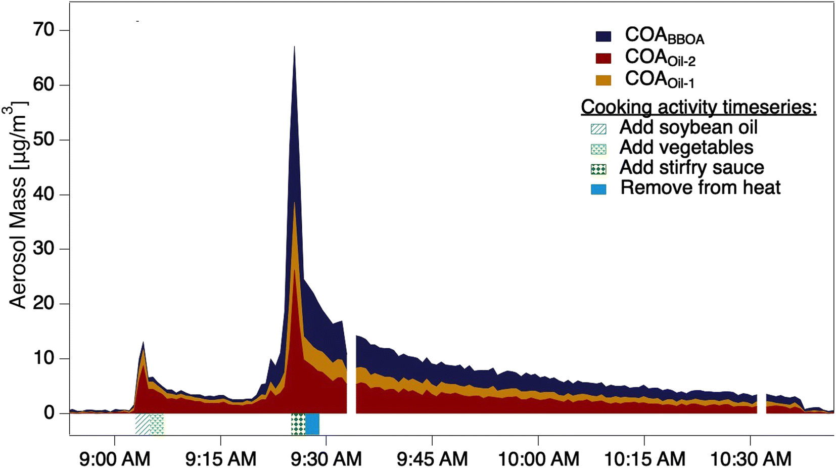 | ||
| Fig. 1 Aerosol mass loading during the control experiment in which stir fry aerosol was sampled without the use of the thermodenuder. Mass loadings for each PMF factor are stacked to show the total organic aerosol mass measured by the ACSM. Shading beneath the plot indicates the timing for each specific cooking activity. | ||
We identified three components of COA as factors using PMF analysis on the nine stir-fries, including measurements with and without the thermal denuder. Based on mass spectral fingerprints and correlations to factors in the literature, we defined the three factors as:
• COABBOA: a biomass burning-like cooking organic aerosol factor that is maximized when the stir-fry sauce is added.
• COAoil-1: a thermally decomposed (and thus more volatile) component of cooking oil.
• COAoil-2: cooking oil aerosol that has undergone little chemical transformation (less volatile than the decomposed component); dominates aerosol after the oil addition to the hot pan.
The biomass-burning-like cooking organic aerosol factor (COABBOA) correlates well with reference mass spectra for BBOA (dot product = 0.81). The dominant ion fragments occur at m/z 29, 44, 60, and 73. The signal at m/z 60 (C2H4O2+) is often attributed to sugars, such as levoglucosan, which can be released during biomass combustion as the products of cellulose pyrolysis (Fig. S8b†). COABBOA contributes little to the total OA mass at the beginning of the stir-fry experiments, but is a substantial fraction of the total OA after the sauce is added. The timing suggests two contributions to COABBOA: thermal decomposition via cooking of vegetable matter and heating of the sauce. Due to the mass spectral similarity of COABBOA to wood smoke and other biomass burning sources, our results suggest that ambient urban measurements of BBOA-like factors may be convoluted with exfiltrated cooking aerosol.
The other two factors are associated with cooking oil, denoted as COAoil-1 and COAoil-2. Due to similar temporal trends, PMF was only able to separate the cooking oil factors due to their differences in volatility, i.e. T50(COAoil-2) > T50(COAoil-1), with the rationale that COAoil-2 has lower volatility than COAoil-1. Non-decomposed cooking oil dominates the total COA mass preceding the oil addition across the nine stir-fries, with on average 64% of the mass belonging to the COAoil-2 factor. When the sauce was added to the wok, COAoil-1 increases to a third of the total COA mass, highlighting the potential for different ingredients to influence cooking aerosol composition. The mass spectra of these two oil factors include fragment ions that repeat every +12 or +14 m/z units, common for long chain hydrocarbon molecules and typical of urban HOA spectra. Both factors appear immediately upon addition of oil to the hot wok and constitute the majority of OA mass until the sauce is added and the COABBOA levels rise. Soybean oil is composed of 51% linoleic, 23% oleic, 10% palmic, 7% linolenic and 4% steric acids by mass; the remaining 5% of soybean oil mass is a combination of other known and unidentified compounds.50 We created a composition-weighted sum mass spectrum of soybean oil using spectra of NIST measured/reported standards for each compound (Fig. S9†); the two oil factors have similar mass spectra to the predicted soybean oil mass spectrum, with the highest signals at m/z 41, 43, 55, 57, and 67, as well as similarly clustered fragments at higher (>70 m/z) masses (Fig. S8c and d†). The two oil-related COA factors are well correlated with the predicted soybean oil mass spectrum, indicating that they are indeed aerosolized, heated cooking oil (dot product = 0.73 for COAoil-2 and = 0.85 for COAoil-1). Based on the mass spectra, we suggest that one factor (COAoil-2) is the result of heating oil and releasing oil-like aerosol, while (COAoil-1) is a thermally decomposed component of cooking oil. COAoil-1 may contain an additional component of decomposed triglycerides. Triglycerides are products of esterification of long chain hydrocarbons, have been observed in films resulting from cooking oil deposition to indoor surfaces,51 and thermally degrade when heated52 at temperatures consistent with the wok during HOMEChem.
3.2 Aerosol volatility
The two stir-fry experiments during which the thermal scan started after the second OA mass concentration peak provided volatility profiles of COA and its three factors (Fig. 2a and S10†). Despite the carefully scripted stir-fry recipe, precision in timing and cooking style affected OA emissions. For example, stir-fry 1 (Fig. 2a) used 4.5 cups of vegetables rather than the scripted amount of 6 cups, and recorded a wok temperature prior to sauce addition of 71 °C. Stir-fry 2 (Fig. S10†) used 6 cups of vegetables and recorded a wok temp of 82 °C prior to sauce addition. The length of time between heating the wok and adding cooking oil may also vary across stir-fries: while the timing is unclear for stir-fry 1, stir-fry 2 had two minutes of cooking oil in the wok before adding vegetables, and recorded an oil temperature of 177 °C just prior to vegetable addition.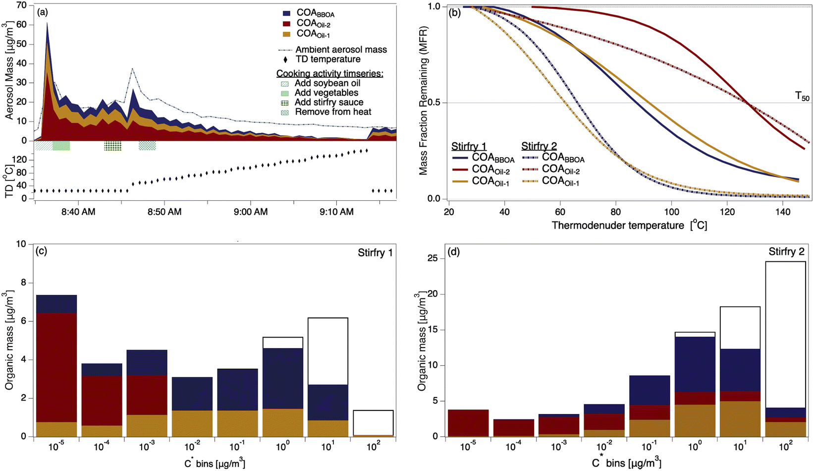 | ||
| Fig. 2 (a) The timeseries of aerosol during a thermal scanning experiment; the dashed line shows the total sub-micron aerosol loading measured by the POPS. The lower part of (a) shows the thermodenuder temperature. (b) Thermograms of the COA factors from two stir-fry experiments; solid trace from stir-fry 1 (shown in (a)), dashed from stir-fry 2, also presented in detail in Fig. S7.† (c) VBS distributions calculated from the thermogram collected during stir-fry 1 (solid trace in (b)). Colored portions indicate mass in the aerosol phase, while colorless portions indicate gas-phase mass. (d) VBS distributions calculated from the thermogram collected during stir-fry 2 (dashed trace in (b)). | ||
We observe considerable experiment-to-experiment variability in volatility for stir-fry emissions; therefore, stir-fry 1 and stir-fry 2 act as a lower and upper bound (in volatility space) for observed stir-fry emissions. While the T50 of each factor varied between experiments (e.g.Fig. 2b), COAoil-2 had a consistently higher T50 – and thus lower volatility – than either COABBOA or COAoil-1, consistent with the identification of the COAoil-1 being thermally decomposed and thus more fragmented than COAoil-2. Comparing the stir-fries, we see the T50 values for stir-fry 1 are higher than their counterparts from stir-fry 2, except for the COAoil-2T50, which is similar for both stir-fry events. The total emitted OA mass during the sauce addition was ∼50% higher during stir-fry 2, likely due to the greater volume of vegetables used in the stir-fry. The fraction of COABBOA + COAoil-1 to total COA were similar for the two stir-fries (61% for stir-fry 2 versus 56% for stir-fry 1). The higher wok temperature during the second stir-fry may account for the slightly higher fraction of BBOA and decomposed oil factors in the COA by enhancing the browning or charring of the vegetables and oil.
Several trends in the volatility of the three COA factors emerge when viewing the VBS profiles for the two experiments (Fig. 2c and d). In both experiments the majority of the mass for both COABBOA and COAoil-1 exists in volatility bins with C* ≥ 0.01 μg m−3, characterizing both factors as semi-volatile. COAoil-2 primarily exists in volatility bins with C* ≤ 0.01 μg m−3, indicating low volatility. For the COABBOA and COAoil-1 factors, higher T50 values from stir-fry 1 (Fig. 2b) mean that the majority of the mass in the VBS (Fig. 2c) is in C* bins ≤0.01 μg m−3 while lower T50 values from stir-fry 2 translates to a portion of the mass in C* bins ≥0.01 μg m−3. Details on the VBS calculation and volatility data from the other experiments not shown here are in the ESI (Section S4, Fig. S12 and S13†).
3.3 Dilution-driven evaporation
Compared to ambient urban COA spectra, the near-source COA measured after the oil addition had a slightly higher correlation than emissions observed after the sauce addition (Table S1†). The lower-volatility oil factor (COAoil-2) is the dominant component of the first COA concentration spike and is also the most similar to literature COA from outdoor urban measurements (dot product = 0.96; Table S1†). Based on this correlation and the VBS of each factor, we hypothesize that while cooking emits multiple types of COA, dilution-driven evaporation can remove the more volatile components, leaving this COAoil-2 to dominate ambient COA. To explore this hypothesis, we use a gas-particle chemical kinetics model to predict the phase state of the COA as it is transported from the emission source within and outside the house.The chemical kinetics model calculates the time-dependent shift of mass from aerosol to gas in a given scenario based on general partitioning theory.26 The model was originally developed by Riipinen et al. (2010)53 and used to describe aerosol partitioning in a thermodenuder (details are provided in ESI Section S5 – Kinetic partitioning model†). We constrained the model with indoor measurements of temperature, aerosol volatility, and size distribution. Details are provided in ESI Section S5 and associated tables and figures.† Air in the kitchen area is assumed to be well mixed during the stir-fry. The model dilutes the aerosol mass in two steps, first as the aerosol mixes through the house, and second as the aerosol is exfiltrated into the outdoor atmosphere. Outdoors, we consider two scenarios based on ambient measurements taken during HOMEChem: (1) clean air with sub-micron OA mass loading of 5 μg m−3 and (2) mildly polluted air with submicron OA loading of 15 μg m−3. These ranges are consistent with more detailed studies of urban PM in Austin, TX.54 We model the fate of aerosol emitted in the kitchen considering three volatility profiles: (1) aerosol with the VBS in Fig. 2c (lower bound volatility); (2) aerosol with the VBS in Fig. 2d (higher bound volatility); and (3) aerosol with a VBS of near-source vehicle emissions.55 In all cases, we assume air temperature is constant at 25 °C through the entire house and outside. Thus, any mass loss is driven solely by dilution-driven evaporation. It has been previously shown that deposition and exfiltration (not including venting through window- or door-opening) are too slow to account for spatial variations in particle concentration throughout a house, making dilution the dominate driver of these spatial variations.56 For simplicity, we therefore assume no losses from deposition or exfiltration. These assumptions mean that our estimates of dilution-driven evaporation should be considered lower bounds; more losses would cause decreased aerosol concentrations and thus increased evaporation if the volatility distribution remains unchanged.
The initial dilution from the kitchen through the house evaporated a substantial fraction (∼24%) of the COA (Fig. 3 and S15†). Transport and dilution to the outdoor atmosphere further evaporated the initial emissions, losing ∼30–60% of the total original COA mass via dilution-driven evaporation. Most of the evaporated mass is from the more volatile components COABBOA and COAoil-1 (Fig. 3), meaning that the chemical composition of COA shifts as the particles dilute through the house and outdoors, with the total COA becoming more similar to COAoil-2. This model result is consistent with our hypothesis that primary COA observed in regional aerosol would appear more like this lower volatility factor, as observed by Paciga et al.29 However, while this dilution-driven evaporation substantially reduces aerosol mass in the house, it is unlikely to have a strong impact on indoor gas-phase organic budgets. To that end, Mattila et al.57 compiled a reactive organic carbon budget and found that organic compounds in the particle phase contribute only a minor fraction of total organic carbon in indoor air, even during cooking events.
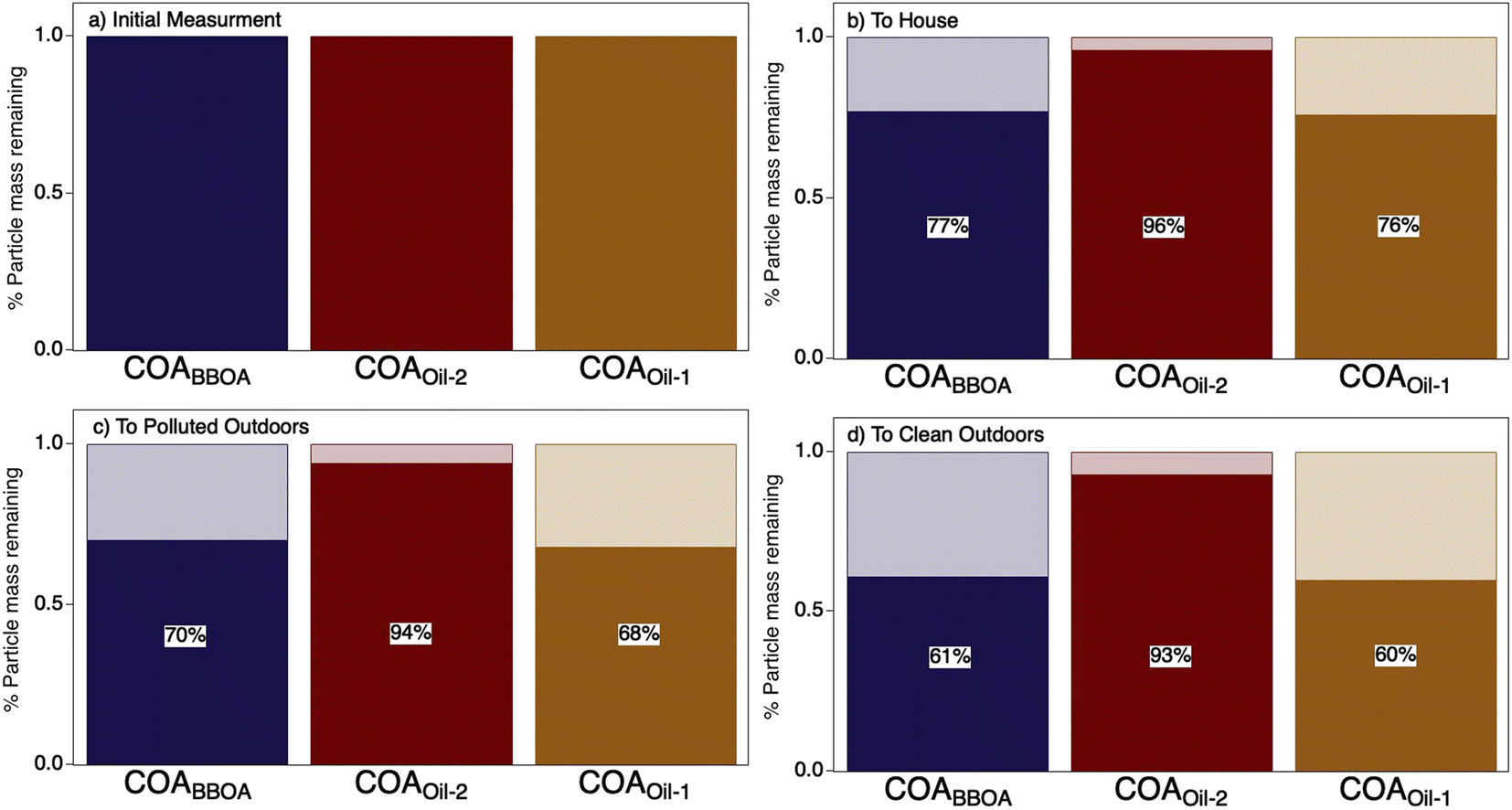 | ||
| Fig. 3 Results from a chemical kinetic partitioning model describing the dilution-driven evaporation of aerosol emitted during a stir-fry experiment (same experiment as represented in Fig. 2d). Bar charts show the fraction of mass remaining (solid) for each COA factor due to dilution-driven evaporation upon reaching thermodynamic equilibrium for (a) the initial emission, (b) after mixing throughout the volume of the residence, (c) after exfiltration outdoors on a more polluted day in Austin TX, and (d) on a cleaner day in Austin, TX. The initial mass concentration for each factor in (a) are provided in ESI Table S4† and percent particulate mass remaining (b–d) is provided on top of the bar charts. | ||
This evaporated organic matter has several fates in both the indoor and outdoor environments: contributing to gas-phase organic carbon, depositing to surfaces, or acting as reactants for oxidation or other chemical transformations. Deposition of COA and its derived gases to indoor environments may contribute to the large organic surface reservoirs predicted to exist throughout the house.58 Gas-phase oxidation in indoor environments occurs in polluted urban environments and is enhanced by window opening, cleaning with oxidative products,59 and other manipulations like ozone-producing air cleaners or other devices.60 Gas-phase oxidation also occurs outdoors. For example, recent work showed that near-field smoke emissions undergo substantial dilution-driven evaporation, but that subsequent gas-phase oxidation of evaporated mass formed secondary organic aerosol, resulting in little net change in total organic aerosol as the plume aged.61–63 The extent to which COA gases are oxidized and contribute to SOA formation in urban settings warrants further study.
Due to a lack of data availability and because both cooking and vehicle emissions are primary sources that are dominated by hydrocarbons, previous literature has used vehicle exhaust to predict cooking volatility.8,64 However, Fig. 4 shows that vehicle emissions have mass in higher C* bins (C* ≥ 0.01 μg m−3), and are thus more volatile than COA. Interestingly, vehicle exhaust is similar to the summed COABBOA + COAoil-1 portions of the total COA emissions, excluding COAoil-2. Thus, vehicle organic aerosol is more volatile than COA, and will undergo more dilution-driven evaporation in the atmosphere. Where the vehicle VBS loses 58% of its aerosol mass upon dilution to the outdoor air (low loading), the HOMEChem COA (low loading) loses only 13–38% of its aerosol mass, with the range driven by variability in VBS calculated from the different stir-fry experiments. However, chemical transport models that are typically used to investigate urban and regional air quality would only consider the emission to the outdoor atmosphere (i.e. COA upon exfiltration), and the impact of using VBS profiles for COA that are too volatile relative to the initial emission may be diminished. However, this contrast suggests that chemical transport models may need to treat indoor and outdoor cooking emissions separately to accurately capture their impact on ambient aerosol levels.
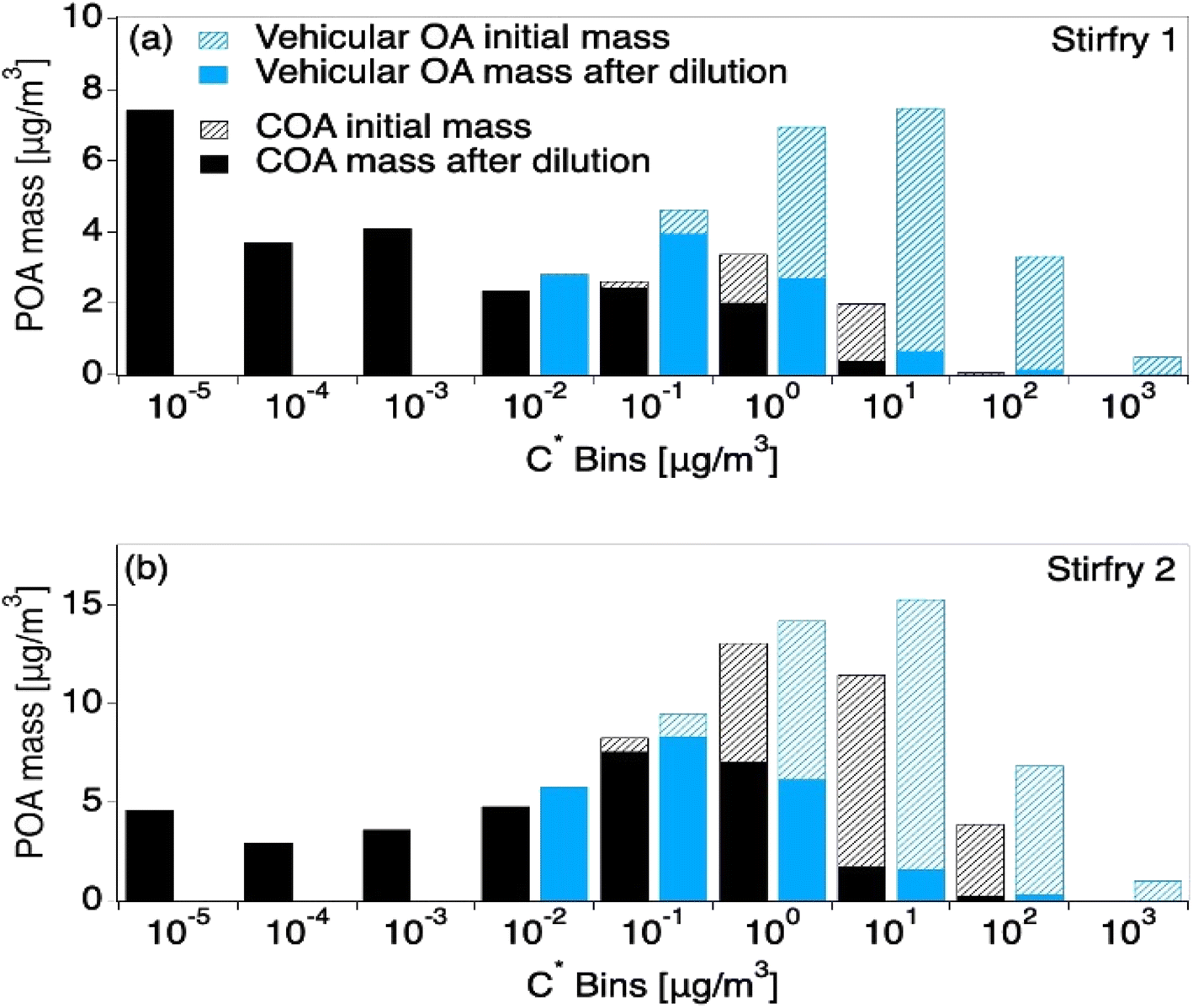 | ||
| Fig. 4 Model results from two HOMEChem stir-fry experiments after being transported outdoors in the clean atmosphere scenario, contrasting VBS derived from observations versus VBS from vehicle emissions, which are sometimes used as a proxy for COA. Model inputs are held constant except for mass in each C* bin, which come from the VBS. Hash portions of each distribution represent the mass lost to dilution-driven evaporation after the aerosol has reached thermodynamic equilibrium with the outside atmosphere. The top panel (a) shows the VBS derived from the first stir-fry, which results in lower-volatility COA described in Fig. 2c. The lower panel (b) shows the second, higher-volatility stir-fry described in Fig. 2d. | ||
4. Conclusions
Recent work in urban areas has demonstrated the growing importance of volatile chemical products to outdoor air quality in North American cities.6,65 Indoor cooking is another potentially relevant pollution source, releasing both organic particles and gases. Here, we provide a comprehensive characterization of cooking organic aerosol (COA) emissions from stir-fry preparation during a field campaign. These emissions are substantial and contain three chemical factors consistently: one representative of biomass-burning (COABBOA) and two from soybean cooking oil (COAoil-2, COAoil-1). The least volatile component (COAoil-2) was the most similar to previous urban measurements of COA, consistent with our hypothesis and model showing that dilution-driven evaporation influences the composition of cooking aerosol observed in the outdoor atmosphere. However, our observation of a cooking factor that is chemically similar to biomass burning organic aerosol suggests that some urban BBOA signals in aerosol mass spectrometry observations may include a food cooking sources in addition to wood smoke and other contributing sources. Despite carefully scripted activities following just one stir-fry recipe, the volatility profiles of COA varied substantially, highlighting the need for further studies of the composition and volatility of other cooking sources. Such measurements are essential for better predicting the contribution of indoor cooking to outdoor urban air pollution – not just in North America, but also urban areas around the globe as cooking is ubiquitous. This work shows that the fate of cooking organic aerosol brings this pollutant not just throughout the indoor environment, but also outdoors. We calculated a movement of a quarter of the particulate mass to the gas phase through dilution-driven evaporation indoors; for particles that exfiltrate from indoors to outdoors, we calculate a further 6–36% of the initial mass is lost to dilution-driven evaporation outdoors. The remaining primary COA is lower-volatility, but the gases released into the outdoor atmosphere through evaporation can contribute to secondary chemistry, perhaps even returning to the aerosol phase. Cooking must be considered an air pollution source not just through primary emissions of gases and aerosol, but also through the dilution-driven evaporation of mass as particles transport away from the source.Conflicts of interest
There are no conflicts of interest.Acknowledgements
We thank the Alfred P. Sloan Foundation for funding HOMEChem (G-2017-9944) and continued analysis (G-2020-13929), Prof. Atila Novoselac and Dr Steve Bourne for operating the test house; the HOMEChem Science Team for support; and Prof. Jose Jimenez and Dr Doug Day for lending us the thermodenuder. Jeffrey R. Pierce acknowledges funding from the NOAA grant NA21OAR4310128.References
- A. H. Goldstein and I. E. Galbally, Known and Unexplored Organic Constituents in the Earth's Atmosphere, Environ. Sci. Technol., 2007, 41(5), 1514–1521, DOI:10.1021/es072476p.
- B. Yuan, M. Shao, J. de Gouw, D. D. Parrish, S. Lu, M. Wang, L. Zeng, Q. Zhang, Y. Song, J. Zhang and M. Hu, Volatile Organic Compounds (VOCs) in Urban Air: How Chemistry Affects the Interpretation of Positive Matrix Factorization (PMF) Analysis, J. Geophys. Res.: Atmos., 2012, 117(D24) DOI:10.1029/2012JD018236.
- Y. Song, W. Dai, M. Shao, Y. Liu, S. Lu, W. Kuster and P. Goldan, Comparison of Receptor Models for Source Apportionment of Volatile Organic Compounds in Beijing, China, Environ. Pollut., 2008, 156(1), 174–183, DOI:10.1016/j.envpol.2007.12.014.
- Y. Liu, M. Song, X. Liu, Y. Zhang, L. Hui, L. Kong, Y. Zhang, C. Zhang, Y. Qu, J. An, D. Ma, Q. Tan and M. Feng, Characterization and Sources of Volatile Organic Compounds (VOCs) and Their Related Changes during Ozone Pollution Days in 2016 in Beijing, China, Environ. Pollut., 2020, 257, 113599, DOI:10.1016/j.envpol.2019.113599.
- A. K. H. Lau, Z. Yuan, J. Z. Yu and P. K. K. Louie, Source Apportionment of Ambient Volatile Organic Compounds in Hong Kong, Sci. Total Environ., 2010, 408(19), 4138–4149, DOI:10.1016/j.scitotenv.2010.05.025.
- B. C. McDonald, J. A. de Gouw, J. B. Gilman, S. H. Jathar, A. Akherati, C. D. Cappa, J. L. Jimenez, J. Lee-Taylor, P. L. Hayes, S. A. McKeen, Y. Y. Cui, S.-W. Kim, D. R. Gentner, G. Isaacman-VanWertz, A. H. Goldstein, R. A. Harley, G. J. Frost, J. M. Roberts, T. B. Ryerson and M. Trainer, Volatile Chemical Products Emerging as Largest Petrochemical Source of Urban Organic Emissions, Science, 2018, 359(6377), 760–764, DOI:10.1126/science.aaq0524.
- M. Hallquist, J. C. Wenger, U. Baltensperger, Y. Rudich, D. Simpson, M. Claeys, J. Dommen, N. M. Donahue, C. George, A. H. Goldstein, J. F. Hamilton, H. Herrmann, T. Hoffmann, Y. Iinuma, M. Jang, M. E. Jenkin, J. L. Jimenez, A. Kiendler-Scharr, W. Maenhaut, G. McFiggans, T. F. Mentel, A. Monod, A. S. H. Prévôt, J. H. Seinfeld, J. D. Surratt, R. Szmigielski and J. Wildt, The Formation, Properties and Impact of Secondary Organic Aerosol: Current and Emerging Issues, Atmos. Chem. Phys., 2009, 9(14), 5155–5236, DOI:10.5194/acp-9-5155-2009.
- P. L. Hayes, A. G. Carlton, K. R. Baker, R. Ahmadov, R. A. Washenfelder, S. Alvarez, B. Rappenglück, J. B. Gilman, W. C. Kuster, J. A. de Gouw, P. Zotter, A. S. H. Prévôt, S. Szidat, T. E. Kleindienst, J. H. Offenberg, P. K. Ma and J. L. Jimenez, Modeling the Formation and Aging of Secondary Organic Aerosols in Los Angeles during CalNex 2010, Atmos. Chem. Phys., 2015, 15(10), 5773–5801, DOI:10.5194/acp-15-5773-2015.
- C. L. Heald and J. H. Kroll, The Fuel of Atmospheric Chemistry: Toward a Complete Description of Reactive Organic Carbon, Sci. Adv., 2020, 6(6), 1–9, DOI:10.1126/sciadv.aay8967.
- N. M. Donahue, A. L. Robinson and S. N. Pandis, Atmospheric Organic Particulate Matter: From Smoke to Secondary Organic Aerosol, Atmos. Environ., 2009, 43(1), 94–106, DOI:10.1016/j.atmosenv.2008.09.055.
- N. M. Donahue, A. L. Robinson, E. R. Trump, I. Riipinen and J. H. Kroll, in Volatility and Aging of Atmospheric Organic Aerosol, Springer-Verlag Berlin Heidelberg, 2012, vol. 310, pp. 97–143, DOI:10.1007/128_2012_355.
- W. L. Brown, D. A. Day, H. Stark, D. Pagonis, J. E. Krechmer, X. Liu, D. J. Price, E. F. Katz, P. F. DeCarlo, C. G. Masoud, D. S. Wang, L. Hildebrandt Ruiz, C. Arata, D. M. Lunderberg, A. H. Goldstein, D. K. Farmer, M. E. Vance and J. L. Jimenez, Real-Time Organic Aerosol Chemical Speciation in the Indoor Environment Using Extractive Electrospray Ionization Mass Spectrometry, Indoor Air, 2021, 31(1), 141–155, DOI:10.1111/ina.12721.
- E. F. Katz, H. Guo, P. Campuzano-Jost, D. A. Day, W. L. Brown, E. Boedicker, M. Pothier, D. M. Lunderberg, S. Patel, K. Patel, P. L. Hayes, A. Avery, L. Hildebrandt Ruiz, A. H. Goldstein, M. E. Vance, D. K. Farmer, J. L. Jimenez and P. F. DeCarlo, Quantification of Cooking Organic Aerosol in the Indoor Environment Using Aerodyne Aerosol Mass Spectrometers, Aerosol Sci. Technol., 2021, 55(10), 1099–1114, DOI:10.1080/02786826.2021.1931013.
- T. Liu, Z. Wang, D. D. Huang, X. Wang and C. K. Chan, Significant Production of Secondary Organic Aerosol from Emissions of Heated Cooking Oils, Environ. Sci. Technol. Lett., 2018, 5(1), 32–37, DOI:10.1021/acs.estlett.7b00530.
- L.-Y. He, Y. Lin, X.-F. Huang, S. Guo, L. Xue, Q. Su, M. Hu, S.-J. Luan and Y.-H. Zhang, Characterization of High-Resolution Aerosol Mass Spectra of Primary Organic Aerosol Emissions from Chinese Cooking and Biomass Burning, Atmos. Chem. Phys., 2010, 10(23), 11535–11543, DOI:10.5194/acp-10-11535-2010.
- D. Allan, P. I. Williams, W. T. Morgan, C. L. Martin, M. J. Flynn, J. Lee, E. Nemitz, G. J. Phillips, M. W. Gallagher and H. Coe, Contributions from Transport, Solid Fuel Burning and Cooking to Primary Organic Aerosols in Two UK Cities, Atmos. Chem. Phys., 2010, 10(2), 647–668, DOI:10.5194/acp-10-647-2010.
- X. F. Huang, L. Y. He, M. Hu, M. R. Canagaratna, Y. Sun, Q. Zhang, T. Zhu, L. Xue, L. W. Zeng, X. G. Liu, Y. H. Zhang, J. T. Jayne, N. L. Ng and D. R. Worsnop, Highly Time-Resolved Chemical Characterization of Atmospheric Submicron Particles during 2008 Beijing Olympic Games Using an Aerodyne High-Resolution Aerosol Mass Spectrometer, Atmos. Chem. Phys., 2010, 10(18), 8933–8945, DOI:10.5194/acp-10-8933-2010.
- Y. Sun, Z. Wang, H. Dong, T. Yang, J. Li, X. Pan, P. Chen and J. T. Jayne, Characterization of Summer Organic and Inorganic Aerosols in Beijing, China with an Aerosol Chemical Speciation Monitor, Atmos. Environ., 2012, 51, 250–259, DOI:10.1016/j.atmosenv.2012.01.013.
- Y.-L. Sun, Q. Zhang, J. J. Schwab, K. L. Demerjian, W.-N. Chen, M.-S. Bae, H.-M. Hung, O. Hogrefe, B. Frank, O. V. Rattigan and Y.-C. Lin, Characterization of the Sources and Processes of Organic and Inorganic Aerosols in New York City with a High-Resolution Time-of-Flight Aerosol Mass Apectrometer, Atmos. Chem. Phys., 2011, 11(4), 1581–1602, DOI:10.5194/acp-11-1581-2011.
- M. Crippa, P. F. Decarlo, J. G. Slowik, C. Mohr, M. F. Heringa, R. Chirico, L. Poulain, F. Freutel, J. Sciare, J. Cozic, C. F. Di Marco, M. Elsasser, J. B. Nicolas, N. Marchand, E. Abidi, A. Wiedensohler, F. Drewnick, J. Schneider, S. Borrmann, E. Nemitz, R. Zimmermann, J. L. Jaffrezo, A. S. H. Prévôt and U. Baltensperger, Wintertime Aerosol Chemical Composition and Source Apportionment of the Organic Fraction in the Metropolitan Area of Paris, Atmos. Chem. Phys., 2013, 13(2), 961–981, DOI:10.5194/acp-13-961-2013.
- W. Xu, C. Xie, E. Karnezi, Q. Zhang, J. Wang, S. N. Pandis, X. Ge, J. Zhang, J. An, Q. Wang, J. Zhao, W. Du, Y. Qiu, W. Zhou, Y. He, Y. Li, J. Li, P. Fu, Z. Wang, D. R. Worsnop and Y. Sun, Summertime Aerosol Volatility Measurements in Beijing, China, Atmos. Chem. Phys., 2019, 19(15), 10205–10216, DOI:10.5194/acp-19-10205-2019.
- M. Takhar, Y. Li and A. W. H. Chan, Characterization of Secondary Organic Aerosol from Heated-Cooking-Oil Emissions: Evolution in Composition and Volatility, Atmos. Chem. Phys., 2021, 21(6), 5137–5149, DOI:10.5194/acp-21-5137-2021.
- N. M. Donahue, A. L. Robinson, C. O. Stanier and S. N. Pandis, Coupled Partitioning, Dilution, and Chemical Aging of Semivolatile Organics, Environ. Sci. Technol., 2006, 40(8), 2635–2643, DOI:10.1021/es052297c.
- N. M. Donahue, S. A. Epstein, S. N. Pandis and A. L. Robinson, A Two-Dimensional Volatility Basis Set: 1. Organic-Aerosol Mixing Thermodynamics, Atmos. Chem. Phys., 2011, 11(7), 3303–3318, DOI:10.5194/acp-11-3303-2011.
- N. M. Donahue, J. H. Kroll, S. N. Pandis and A. L. Robinson, A Two-Dimensional Volatility Basis Set – Part 2: Diagnostics of Organic-Aerosol Evolution, Atmos. Chem. Phys., 2012, 12(2), 615–634, DOI:10.5194/acp-12-615-2012.
- J. F. Pankow, An Absorption Model of Gas/Particle Partitioning of Organic Compounds in the Atmosphere, Atmos. Environ., 1994, 28(2), 185–188, DOI:10.1016/1352-2310(94)90093-0.
- S. A. Epstein, I. Riipinen and N. M. Donahue, A Semiempirical Correlation between Enthalpy of Vaporization and Saturation Concentration for Organic Aerosol, Environ. Sci. Technol., 2010, 44(2), 743–748, DOI:10.1021/es902497z.
- C. D. Cappa and J. L. Jimenez, Quantitative Estimates of the Volatility of Ambient Organic Aerosol, Atmos. Chem. Phys., 2010, 10(12), 5409–5424, DOI:10.5194/acp-10-5409-2010.
- A. Paciga, E. Karnezi, E. Kostenidou, L. Hildebrandt, M. Psichoudaki, G. J. Engelhart, B. H. Lee, M. Crippa, A. S. H. Prévôt, U. Baltensperger and S. N. Pandis, Volatility of Organic Aerosol and Its Components in the Megacity of Paris, Atmos. Chem. Phys., 2016, 16(4), 2013–2023, DOI:10.5194/acp-16-2013-2016.
- M. Takhar, C. A. Stroud and A. W. H. Chan, Volatility Distribution and Evaporation Rates of Organic Aerosol from Cooking Oils and Their Evolution upon Heterogeneous Oxidation, ACS Earth Space Chem., 2019, 1717–1728, DOI:10.1021/acsearthspacechem.9b00110.
- J. A. Huffman, K. S. Docherty, C. Mohr, M. J. Cubison, I. M. Ulbrich, P. J. Ziemann, T. B. Onasch and J. L. Jimenez, Chemically-Resolved Volatility Measurements of Organic Aerosol from Different Sources, Environ. Sci. Technol., 2009, 43(14), 5351–5357, DOI:10.1021/es803539d.
- E. E. Louvaris, E. Karnezi, E. Kostenidou, C. Kaltsonoudis and S. N. Pandis, Estimation of the Volatility Distribution of Organic Aerosol Combining Thermodenuder and Isothermal Dilution Measurements, Atmos. Meas. Tech., 2017, 10(10), 3909–3918, DOI:10.5194/amt-10-3909-2017.
- Y. Morino, T. Nagashima, S. Sugata, K. Sato, K. Tanabe, T. Noguchi, A. Takami, H. Tanimoto and T. Ohara, Verification of Chemical Transport Models for PM2.5 Chemical Composition Using Simultaneous Measurement Data over Japan, Aerosol Air Qual. Res., 2015, 15(5), 2009–2023, DOI:10.4209/aaqr.2015.02.0120.
- K. C. Barsanti, A. G. Carlton and S. H. Chung, Analyzing Experimental Data and Model Parameters: Implications for Predictions of SOA Using Chemical Transport Models, Atmos. Chem. Phys., 2013, 13(23), 12073–12088, DOI:10.5194/acp-13-12073-2013.
- R. Bergström, H. A. C. Denier van der Gon, A. S. H. Prévôt, K. E. Yttri and D. Simpson, Modelling of Organic Aerosols over Europe (2002–2007) Using a Volatility Basis Set (VBS) Framework: Application of Different Assumptions Regarding the Formation of Secondary Organic Aerosol, Atmos. Chem. Phys., 2012, 12(18), 8499–8527, DOI:10.5194/acp-12-8499-2012.
- V. Lannuque, F. Couvidat, M. Camredon, B. Aumont and B. Bessagnet, Modelling Organic Aerosol over Europe in Summer Conditions with the VBS-GECKO Parameterization: Sensitivity to Secondary Organic Compound Properties and IVOC Emissions, Atmos. Chem. Phys., 2019, 1–40, DOI:10.5194/acp-2018-1244.
- S. N. Pandis, N. M. Donahue, B. N. Murphy, I. Riipinen, C. Fountoukis, E. Karnezi, D. Patoulias and K. Skyllakou, Introductory Lecture: Atmospheric Organic Aerosols: Insights from the Combination of Measurements and Chemical Transport Models, Faraday Discuss., 2013, 165, 9, 10.1039/c3fd00108c.
- I. M. Ulbrich, M. R. Canagaratna, Q. Zhang, D. R. Worsnop and J. L. Jimenez, Interpretation of Organic Components from Positive Matrix Factorization of Aerosol Mass Spectrometric Data, Atmos. Chem. Phys., 2009, 9(9), 2891–2918, DOI:10.5194/acp-9-2891-2009.
- Q. Zhang, J. L. Jimenez, M. R. Canagaratna, I. M. Ulbrich, N. L. Ng, D. R. Worsnop and Y. Sun, Understanding Atmospheric Organic Aerosols via Factor Analysis of Aerosol Mass Spectrometry: A Review, Anal. Bioanal. Chem., 2011, 401(10), 3045–3067, DOI:10.1007/s00216-011-5355-y.
- M. R. Canagaratna, T. B. Onasch, E. C. Wood, S. C. Herndon, J. T. Jayne, E. S. Cross, R. C. Miake-Lye, C. E. Kolb and D. R. Worsnop, Evolution of Vehicle Exhaust Particles in the Atmosphere, J. Air Waste Manage. Assoc., 2010, 60(10), 1192–1203, DOI:10.3155/1047-3289.60.10.1192.
- M. R. Canagaratna, J. L. Jimenez, J. H. Kroll, Q. Chen, S. H. Kessler, P. Massoli, L. Hildebrandt Ruiz, E. Fortner, L. R. Williams, K. R. Wilson, J. D. Surratt, N. M. Donahue, J. T. Jayne and D. R. Worsnop, Elemental Ratio Measurements of Organic Compounds Using Aerosol Mass Spectrometry: Characterization, Improved Calibration, and Implications, Atmos. Chem. Phys., 2015, 15(1), 253–272, DOI:10.5194/acp-15-253-2015.
- D. M. Lunderberg, K. Kristensen, Y. Tian, C. Arata, P. K. Misztal, Y. Liu, N. Kreisberg, E. F. Katz, P. F. Decarlo, S. Patel, M. E. Vance, W. W. Nazaroff and A. H. Goldstein, Surface Emissions Modulate Indoor SVOC Concentrations through Volatility-Dependent Partitioning, Environ. Sci. Technol., 2020, 54(11), 6751–6760, DOI:10.1021/acs.est.0c00966.
- S. Patel, S. Sankhyan, E. K. Boedicker, P. F. Decarlo, D. K. Farmer, A. H. Goldstein, E. F. Katz, W. W. Nazaroff, Y. Tian, J. Vanhanen and M. E. Vance, Indoor Particulate Matter during HOMEChem: Concentrations, Size Distributions, and Exposures, Environ. Sci. Technol., 2020, 54(12), 7107–7116, DOI:10.1021/acs.est.0c00740.
- Y. Tian, C. Arata, E. Boedicker, D. M. Lunderberg, S. Patel, S. Sankhyan, K. Kristensen, P. K. Misztal, D. K. Farmer, M. Vance, A. Novoselac, W. W. Nazaroff and A. H. Goldstein, Indoor Emissions of Total and Fluorescent Supermicron Particles during HOMEChem, Indoor Air, 2021, 31(1), 88–98, DOI:10.1111/ina.12731.
- J. A. Huffman, P. J. Ziemann, J. T. Jayne, D. R. Worsnop and J. L. Jimenez, Development and Characterization of a Fast-Stepping/Scanning Thermodenuder for Chemically-Resolved Aerosol Volatility Measurements, Aerosol Sci. Technol., 2008, 42(5), 395–407, DOI:10.1080/02786820802104981.
- R. Fröhlich, M. J. Cubison, J. G. Slowik, N. Bukowiecki, A. S. H. Prévôt, U. Baltensperger, J. Schneider, J. R. Kimmel, M. Gonin, U. Rohner, D. R. Worsnop and J. T. Jayne, The ToF-ACSM: A Portable Aerosol Chemical Speciation Monitor with TOFMS Detection, Atmos. Meas. Tech., 2013, 6(11), 3225–3241, DOI:10.5194/amt-6-3225-2013.
- D. K. Farmer, M. E. Vance, J. P. D. Abbatt, A. Abeleira, M. R. Alves, C. Arata, E. Boedicker, S. Bourne, F. Cardoso-Saldaña, R. Corsi, P. F. Decarlo, A. H. Goldstein, V. H. Grassian, L. Hildebrandt Ruiz, J. L. Jimenez, T. F. Kahan, E. F. Katz, J. M. Mattila, W. W. Nazaroff, A. Novoselac, R. E. O'Brien, V. W. Or, S. Patel, S. Sankhyan, P. S. Stevens, Y. Tian, M. Wade, C. Wang, S. Zhou and Y. Zhou, Overview of HOMEChem: House Observations of Microbial and Environmental Chemistry, Environ. Sci.: Processes Impacts, 2019, 21(8), 1280–1300, 10.1039/c9em00228f.
- A. E. Faulhaber, B. M. Thomas, J. L. Jimenez, J. T. Jayne, D. R. Worsnop and P. J. Ziemann, Characterization of a Thermodenuder-Particle Beam Mass Spectrometer System for the Study of Organic Aerosol Volatility and Composition, Atmos. Meas. Tech., 2009, 2(1), 15–31, DOI:10.5194/amt-2-15-2009.
- R. S. Gao, H. Telg, R. J. McLaughlin, S. J. Ciciora, L. A. Watts, M. S. Richardson, J. P. Schwarz, A. E. Perring, T. D. Thornberry, A. W. Rollins, M. Z. Markovic, T. S. Bates, J. E. Johnson and D. W. Fahey, A Light-Weight, High-Sensitivity Particle Spectrometer for PM2.5 Aerosol Measurements, Aerosol Sci. Technol., 2016, 50(1), 88–99, DOI:10.1080/02786826.2015.1131809.
- F. D. Gunstone, The Major Sources of Oils, Fats, and Other Lipids, in Fatty Acid and Lipid Chemistry, ed. Gunstone, F. D., Springer US, Boston, MA, 1996, pp. 61–86, DOI:10.1007/978-1-4615-4131-8_3.
- R. E. O'Brien, Y. Li, K. J. Kiland, E. F. Katz, V. W. Or, E. Legaard, E. Q. Walhout, C. Thrasher, V. H. Grassian, P. F. Decarlo, A. K. Bertram and M. Shiraiwa, Emerging Investigator Series: Chemical and Physical Properties of Organic Mixtures on Indoor Surfaces during HOMEChem, Environ. Sci.: Processes Impacts, 2021, 23(4), 559–568, 10.1039/d1em00060h.
- S. Vecchio, L. Campanella, A. Nuccilli and M. Tomassetti, Kinetic Study of Thermal Breakdown of Triglycerides Contained in Extra-Virgin Olive Oil, J. Therm. Anal. Calorim., 2008, 91(1), 51–56, DOI:10.1007/s10973-007-8373-4.
- I. Riipinen, J. R. Pierce, N. M. Donahue and S. N. Pandis, Equilibration Time Scales of Organic Aerosol inside Thermodenuders: Evaporation Kinetics versus Thermodynamics, Atmos. Environ., 2010, 44(5), 597–607, DOI:10.1016/j.atmosenv.2009.11.022.
- K. Patel, D. Wang, P. Chhabra, J. Bean, S. V. Dhulipala and L. Hildebrandt Ruiz, Effects of Sources and Meteorology on Ambient Particulate Matter in Austin, Texas, ACS Earth Space Chem., 2020, 4(4), 602–613, DOI:10.1021/acsearthspacechem.0c00016.
- D. R. Worton, G. Isaacman, D. R. Gentner, T. R. Dallmann, A. W. H. Chan, C. Ruehl, T. W. Kirchstetter, K. R. Wilson, R. A. Harley and A. H. Goldstein, Lubricating Oil Dominates Primary Organic Aerosol Emissions from Motor Vehicles, Environ. Sci. Technol., 2014, 48(7), 3698–3706, DOI:10.1021/es405375j.
- E. K. Boedicker, E. W. Emerson, G. R. McMeeking, S. Patel, M. E. Vance and D. K. Farmer, Fates and Spatial Variations of Accumulation Mode Particles in a Multi-Zone Indoor Environment during the HOMEChem Campaign, Environ. Sci.: Processes Impacts, 2021, 23(7), 1029–1039, 10.1039/D1EM00087J.
- J. M. Mattila, C. Arata, A. Abeleira, Y. Zhou, C. Wang, E. F. Katz, A. H. Goldstein, J. P. D. Abbatt, P. F. DeCarlo, M. E. Vance and D. K. Farmer, Contrasting Chemical Complexity and the Reactive Organic Carbon Budget of Indoor and Outdoor Air, Environ. Sci. Technol., 2022, 56(1), 109–118, DOI:10.1021/acs.est.1c03915.
- C. Wang, D. B. Collins, C. Arata, A. H. Goldstein, J. M. Mattila, D. K. Farmer, L. Ampollini, P. F. Decarlo, A. Novoselac, M. E. Vance, W. W. Nazaroff and J. P. D. Abbatt, Surface Reservoirs Dominate Dynamic Gas-Surface Partitioning of Many Indoor Air Constituents, 2020, vol. 6 Search PubMed.
- C. M. F. Rosales, J. Jiang, A. Lahib, B. P. Bottorff, E. K. Reidy, V. Kumar, A. Tasoglou, H. Huber, S. Dusanter, A. Tomas, B. E. Boor and P. S. Stevens, Chemistry and Human Exposure Implications of Secondary Organic Aerosol Production from Indoor Terpene Ozonolysis, Sci. Adv., 2022, 8(8), 1–17, DOI:10.1126/sciadv.abj9156.
- A. Eftekhari, C. F. Fortenberry, B. J. Williams, M. J. Walker, A. Dang, A. Pfaff, N. Ercal and G. C. Morrison, Continuous measurement of reactive oxygen species inside and outside of a residential house during summer, Indoor Air, 2021, 31, 1199–1216, DOI:10.1111/ina.12789.
- Q. Bian, S. H. Jathar, J. K. Kodros, K. C. Barsanti, L. E. Hatch, A. A. May, S. M. Kreidenweis and J. R. Pierce, Secondary Organic Aerosol Formation in Biomass-Burning Plumes: Theoretical Analysis of Lab Studies and Ambient Plumes, Atmos. Chem. Phys., 2017, 17(8), 5459–5475, DOI:10.5194/acp-17-5459-2017.
- L. A. Garofalo, M. A. Pothier, E. J. T. Levin, T. Campos, S. M. Kreidenweis and D. K. Farmer, Emission and Evolution of Submicron Organic Aerosol in Smoke from Wildfires in the Western United States, ACS Earth Space Chem., 2019, 3(7), 1237–1247, DOI:10.1021/acsearthspacechem.9b00125.
- B. B. Palm, Q. Peng, C. D. Fredrickson, B. H. Lee, L. A. Garofalo, M. A. Pothier, S. M. Kreidenweis, D. K. Farmer, R. P. Pokhrel, Y. Shen, S. M. Murphy, W. Permar, L. Hu, T. L. Campos, S. R. Hall, K. Ullmann, X. Zhang, F. Flocke, E. V. Fischer and J. A. Thornton, Quantification of Organic Aerosol and Brown Carbon Evolution in Fresh Wildfire Plumes, Proc. Natl. Acad. Sci. U. S. A., 2020, 117(47), 29469–29477, DOI:10.1073/pnas.2012218117.
- T. Liu, Z. Wang, D. D. Huang, X. Wang and C. K. Chan, Significant Production of Secondary Organic Aerosol from Emissions of Heated Cooking Oils, Environ. Sci. Technol. Lett., 2018, 5(1), 32–37, DOI:10.1021/acs.estlett.7b00530.
- M. M. Coggon, G. I. Gkatzelis, B. C. McDonald, J. B. Gilman, R. H. Schwantes, N. Abuhassan, K. C. Aikin, M. F. Arend, T. A. Berkoff, S. S. Brown, T. L. Campos, R. R. Dickerson, G. Gronoff, J. F. Hurley, G. Isaacman-VanWertz, A. R. Koss, M. Li, S. A. McKeen, F. Moshary, J. Peischl, V. Pospisilova, X. Ren, A. Wilson, Y. Wu, M. Trainer and C. Warneke, Volatile Chemical Product Emissions Enhance Ozone and Modulate Urban Chemistry, Proc. Natl. Acad. Sci. U. S. A., 2021, 118(32), e2026653118, DOI:10.1073/pnas.2026653118.
Footnote |
| † Electronic supplementary information (ESI) available. See DOI: https://doi.org/10.1039/d2em00250g |
| This journal is © The Royal Society of Chemistry 2023 |