
 Open Access Article
 This Open Access Article is licensed under a Creative Commons Attribution-Non Commercial 3.0 Unported Licence
Linking biodegradation kinetics, microbial composition and test temperature – Testing 40 petroleum hydrocarbons using inocula collected in winter and summer†
Karina Knudsmark
Sjøholm
 *a,
Arnaud
Dechesne
a,
Delina
Lyon
b,
David M. V.
Saunders
bc,
Heidi
Birch
a and
Philipp
Mayer
a
*a,
Arnaud
Dechesne
a,
Delina
Lyon
b,
David M. V.
Saunders
bc,
Heidi
Birch
a and
Philipp
Mayer
a
aDepartment of Environmental Engineering, Technical University of Denmark, DK-2800 Kongens Lyngby, Denmark
bConcawe, B-1160 Brussels, Belgium
cShell Health, Shell International B.V., 2596 HR The Hague, The Netherlands
First published on 5th January 2022
Abstract
Many factors affect the biodegradation kinetics of chemicals in test systems and the environment. Empirical knowledge is needed on how much test temperature, inoculum, test substances and co-substrates influence the biodegradation kinetics and microbial composition in the test. Water was sampled from the Gudenaa river in winter (2.7 °C) and summer (17 °C) (microbial inoculum) and combined with an aqueous stock solution of >40 petroleum hydrocarbons prepared by passive dosing. This resulted in low-concentration test systems that were incubated for 30 days at 2.7, 12 and 20 °C. Primary biodegradation kinetics, based on substrate depletion relative to abiotic controls, were determined with automated Solid Phase Microextraction coupled to GC/MS. Biodegradation kinetics were remarkably similar for summer and winter inocula when tested at the same temperature, except when cooling summer inoculum to 2.7 °C which delayed degradation relative to winter inoculum. Amplicon sequencing was applied to determine shifts in the microbial composition between season and during incubations: (1) the microbial composition of summer and winter inocula were remarkably similar, (2) the incubation and the incubation temperature had both a clear impact on the microbial composition and (3) the effect of adding >40 petroleum hydrocarbons at low test concentrations was limited but resulted in some proliferation of the known petroleum hydrocarbon degraders Nevskia and Sulfuritalea. Overall, biodegradation kinetics and its temperature dependency were very similar for winter and summer inoculum, whereas the microbial composition was more affected by incubation and test temperature compared to the addition of test chemicals at low concentrations.
Environmental significanceOne of the most critical properties for the environmental risk assessment of chemicals is persistence, which is normally assessed using standardized biodegradation tests, where microorganisms are decoupled from the environment and incubated at constant test conditions. We conducted experiments with >40 petroleum hydrocarbons at low concentrations to shed light on how inoculum season and test incubations affect biodegradation kinetics and microbial composition. Biodegradation kinetics, temperature dependence and microbial composition were similar for summer and winter inoculum. The decoupling of inoculum from the environment and incubation at constant test conditions affected the microbial composition much more than the presence of test substances. The obtained findings will help understand and reduce the gap between laboratory testing and actual biodegradation in the environment. |
Introduction
Biodegradation kinetics data are essential for the risk and persistency assessment of chemicals and they are a formal regulatory requirement for the registration and use of chemicals on the European market.1,2 Such data are produced in standard laboratory tests, that should ideally be conducted with microorganisms and at conditions that reflect the relevant environment, while at the same time yielding conservative and reproducible data that allow comparisons of biodegradation kinetics between compounds and laboratories.3 A biodegradation test then becomes a compromise between realism, relevance and test specific qualities such as accuracy, precision, reproducibility and well-aligned data.3 Standard test methods are often not suitable for poorly soluble, volatile, or multiconstituent chemicals, (i.e. “difficult to test chemicals”) such as many petroleum hydrocarbons, which then necessitate significant methodological adjustments.4–7 While such adjustments should improve the technical and scientific quality of the tests and their degradation results, they can also lead to regulatory rejection of data. A very recent example of this is the persistency assessment of three ringed alkylated PAHs, where all 18 different biodegradation data sets identified were rejected and this hydrocarbon group was then assessed to be persistent without using the experimental degradation data.8 There is thus an urgent need for the continuous improvement of test methods especially for difficult-to-test substances, while at the same time increasing the mechanistic understanding of how various test factors affect biodegradation kinetics and the microbial composition in the test.9–12The OECD 309 test guideline13 provides ample space for adjustments to specific chemicals or a specific regulatory purpose. We have recently reported test design adjustments for testing primary biodegradation of hydrophobic and (semi)volatile petroleum hydrocarbons.14 Closed headspace vials served as test systems and fully automated Solid Phase Microextraction coupled to GC/MS was then used to measure substrate depletion without opening the vials.4 The tests were conducted at low, environmentally relevant test concentrations in order to avoid solubility limitations, oxygen depletion as well as inhibition of the microbial degraders.5,14,15 Overall, these adjustments made the OECD 309 test better suited for petroleum hydrocarbons that cover a wide range of hydrophobicities and volatilities.5 In addition the hydrocarbons were tested in mixtures in order to generate more and better aligned biodegradation kinetics data,5,14 which also are more environmentally relevant since hydrocarbons co-exist as mixtures in petroleum products and in the environment.15,16
Using this test method, we recently investigated biodegradation kinetics of 43 petroleum hydrocarbons at three test temperatures in water from two geographically distant rivers adapted to different temperatures and climatic conditions. For the two inocula collected from the rivers Danube (Austria, sampled at 12.5 °C) and Gudenaa (Denmark, sampled at 2.7 °C), we found a similar temperature dependency of degradation half-times when tested at the standard temperatures,1,17 12 and 20 °C. This temperature dependency fitted well with the Arrhenius equation.18 The present study was directed to separate the effects of inoculum seasonality and test temperature on the biodegradation kinetics while avoiding the effect of different inoculum sampling locations.
A widely discussed issue is how test conditions affect microbial composition during a biodegradation test. The work by Honti et al.,19 is one of the few studies where biodegradation rates have been generated under both laboratory and field conditions. They found higher biodegradation rates for pharmaceuticals in field experiments. A possible explanation for this observation is the reduced microbial diversity in the laboratory tests compared to field conditions.19 Southwell et al.20 found that both the season of collection and incubation affected the microbial community composition, in a setup where biodegradation was investigated in the OECD 308 and 309 standard tests using inoculum from the same site eight times during a two year period. However, the microbial changes could not clearly be linked to degradation potential of the pesticide isopyrazam.20 The inoculum used in laboratory biodegradation tests is often only characterized based on microbial density (e.g. CFU per mL), whereas the initial microbial composition or its dynamics during tests are rarely investigated.3 It is thus an open question how much the incubation and the standard test conditions modulate the microbial composition. The present study was thus designed to determine changes in microbial composition when changing test temperature, adding test chemicals and separating microbes from the environment (i.e. no nutrient supply etc.).
To investigate some of the main factors potentially impacting biodegradation kinetics and microbial composition we conducted dedicated experiments to link biodegradation kinetics, microbial community composition and test temperature for two inocula sampled at the same site but at different seasons. The biodegradation kinetic data with winter inoculum from Gudenaa (Denmark, sampled at 2.7 °C) was taken from our previous study,18 and was here extended with a new biodegradation data set obtained with summer inoculum from the same location (sampled at 17 °C). The experimental platform developed by Birch et al.4,5 was used to determine compound specific biodegradation kinetics for a large number of hydrocarbons at three test temperatures. DNA extraction and analysis using 16S rRNA gene amplicon sequencing was applied to the river water samples (inocula) and the microbial populations in the tests to investigate differences and changes in microbial community composition.
The specific aims of the present study were to determine (1) seasonal differences in biodegradation half-times of +40 petroleum hydrocarbons by comparing winter inoculum with summer inoculum from the same river, (2) the effect of seasonality on the test temperature dependency of biodegradation kinetics, using our recent study18 and the Arrhenius equation as reference and (3) the effect of test incubation on microbial community composition for a winter and summer inoculum.
Materials and methods
Materials
The same model substances were included as in Sjøholm et al.:18 9,10-dihydroanthracene, phenanthrene, hexachloroethane, 2,3-dimethylheptane, bicyclohexyl, butyldecalin, tetralin, biphenyl, 1,2-dimethylnaphthalene, ethylcyclopentane, 2,6-diisopropylnaphthalene, dibenzothiophene, 3-phenyl-1,1′-bi(cyclohexane) (Sigma Aldrich), 2,4-dimethylheptane, 2,5-dimethylheptane, 3,3-dimethyloctane, 3,5-dimethyloctane, decalin (TCI), dodecylbenzene, dihexyl disulphide, 2,6,10-trimethyldodecane (Chiron) and a mixture obtained from LGC (Middlesex, UK) containing indane, 1,4-diethylbenzene, 1,2-diethylbenzene, 1,2,4,5-tetramethylbenzene (durene), 1,2,3,5-tetramethylbenzene (isodurene), 1-ethyl-2-methyltoluene, 1-ethyl-3-methyltoluene, benzene, n-butylbenzene, ethylbenzene, 4-ethyltoluene, iso-octane, cumene, 1-methylnaphthalene, 2-methylnaphthalene, naphthalene, n-propylbenzene, toluene, 1,2,3-trimethylbenzene, 1,2,4-trimethylbenzene, 1,3,5-trimethylbenzene, m-xylene, o-xylene, and p-xylene (more information on model substances in ESI2†).Translucent silicone rod (3 mm diameter) was ordered custom-made from Altec (altecweb.com, product code 136-8380), and used for passive dosing.21 Solvents used for cleaning and loading the silicone included ethyl acetate (Merck), ethanol (VWR Chemicals), and methanol (Sigma Aldrich). Ultrapure water was produced on an Elga Purelab flex water system from Holm & Halby (Denmark).
Sterile 1 L PET bottles from Bürkle (Mikrolab Aarhus, Denmark) were used for sampling of river water.
Surface water inoculum
Sampling site was chosen based on the following criteria:18 (1) the pre-exposure to petroleum hydrocarbons was minimized by avoiding point sources such as oil refineries, industry, WWTP discharges and larger roads close to or upstream of the sampling site, (2) availability of information on water quality according to the Water Frame Directive (good ecological status, low levels of measured nutrients and pollutants) for the site, and (3) possibility to transport the samples to the laboratory quickly in order to start the experiments within 24 h of sampling. The Gudenaa river in Denmark, between the cities of Ry and Silkeborg, fulfilled these criteria. Exact coordinates for the sampling location are included in Table 1. The Gudenaa is the largest freshwater river in Denmark with a middle water flow capacity of 32.4 m3 s−1.| Parameter | Gudenaa, Denmark 56°6′25′′N 9°43′19′′E | |
|---|---|---|
| Winter, 2019 | Summer, 2020 | |
| 2.7 °C | 17 °C | |
| O2 [mg L−1] | 11.0 | 7.4 |
| pH | 8.3 | 7.7 |
| Conductivity [μS cm−1] | 371 | 280 |
| CFU [mL−1], 24/72 h, 20 °C | 58/1.6 × 103 | 45/1.9 × 103 |
| Total dissolved solids (TDS) [mg L−1] | 150 | 150 |
| Total suspended solids (TSS) [mg L−1] | 0–0.4 | 5.1 ± 0.01 |
| Non-volatile organic carbon (NVOC) [mg L−1] | 4.1 ± 0.1 | 5.6 ± 0.03 |
| PO43− [μg L−1] | 49 ± 0.5 | 34 ± 1 |
| NO2− [μg L−1] | 11.8 ± 0.1 | 8.9 ± 1.1 |
| NH3 [μg L−1] | 57 ± 2.3 | 48 ± 4.8 |
| NO3− [μg L−1] | 2340 ± 13 | 248 ± 38 |
The winter sample was collected January 29th 2019 as described in Sjøholm et al.18 The water temperature at sampling was 2.7 °C and during transportation, the water was kept at 0–3 °C. The summer sample was collected September 16th 2020. At sampling the water temperature was 17 °C and during transportation the temperature was kept at 15.5–16.5 °C. The average temperature the three months before the two sampling events were 5.9 °C and 16.7 °C for the winter and summer sample, respectively.22
Sampling was performed in the free-flowing current of the river, 5–20 cm below the surface. Sampling was performed walking out to 1 m depth in the river, and then 1 L was sampled at a time with a pre-cleaned stainless steel beaker at the end of a 3 m stick. Sampling was performed upstream of the collectors position. The sampled water was distributed in 3 bottles and sampling continued until 12 L were collected. The bottles were packed in an insulated aluminum suitcase, which was filled with insulation material to maintain the sampling temperature during transportation by car. The temperature in the suitcase was logged during transportation. Upon arrival to the laboratory, the sample was stored at the sampling temperature in an incubator. Within 24 h, total suspended solids (TSS), total dissolved solids (TDS), nonvolatile total organic carbon (NVOC), and dissolved nitrogen and phosphate content were determined. Microbial abundance was determined as heterotrophic plate count on R2A agar after 24 and 72 h incubation at 20 °C. Procedures for determining the sample characterization parameters are described in the ESI1† and parameters are given in Table 1.
The content of total suspended solids were low in both samples compared to the ECHA PBT guidance requirements in final decisions on compliance check for the purpose of REACH (10–20 mg L−1).17
Passive dosing to generate test solution
Passive dosing was used to introduce the chemicals into the test without the addition of co-solvent, neat mixture or micro droplets.23 The passive dosing method used here was modified from Birch et al.5 and Hammershøj et al.21 It included three steps: (1) loading of pre-cleaned silicone with the test substances, (2) equilibrating the loaded silicone with pure water (passive dosing), and (3) adding this passive dosing solution (PD solution) to surface water inoculum to prepare biodegradation test systems. Solid test chemicals were loaded to a silicone rod by partitioning from a methanol solution, and liquid test chemicals were loaded to other silicone rods by direct absorption of a mixture of chemicals (∼2% (v/v) of silicone mass). One PD solution was prepared containing the test chemicals that are solid at room temperature and one PD solution containing the test chemicals that are liquid at room temperature. The applied passive dosing method is described in detail in Sjøholm et al.18Biodegradation testing
Biodegradation experiments were carried out at 2.7 °C (sampling temperature for the winter sample), 12 °C and 20 °C. Preparation of test systems followed the procedure described in Birch et al.,5 and are described in detail in Sjøholm et al.18 In brief, 100 μL PD solution containing solid test chemicals, and 650 μL PD solution containing liquid test chemicals were transferred to 14.25 mL surface water (i.e. inoculum) in 20 mL amber glass auto sampler vials, leaving 5 mL headspace in the vial. PD solution was transferred with gas tight Hamilton syringes, and the inoculum was transferred with an Eppendorf multi-pipette. Triplicate biotic test systems were generated for each of eight incubation time points. Abiotic test systems were generated the same way, with ultrapure water instead of surface water inoculum. Each biotic/abiotic pair was prepared from the same passive dosing bottle. Test systems were incubated in temperature-controlled incubators for up to 32 days, and at eight time points, three biotic and three abiotic test systems were transferred from the incubator to the GC autosampler.Chemical analysis
Primary biodegradation was determined based on peak areas of single constituents in biotic relative to abiotic test systems (substrate depletion). Automated Headspace Solid Phase Microextraction (HS-SPME) was performed with a PAL3 autosampler (CTC Analytics, Zwingen, Switzerland) mounted on a Gas Chromatograph coupled to a Mass Spectrometer (GC-MS) (Agilent Technologies 7890B/5977A GC/MSD) and the analytical method is described in detail in Sjøholm et al.18 Analysis was performed on test systems without pre-treatment or conservation. If the test systems were incubated below 20 °C, they were put on the autosampler less than 4 hours before analysis to avoid a temperature change during incubation. Average acquisition time for the three biotic–abiotic pairs of an analysis point was then used as time point in the further data treatment.Data treatment
The analytical method was successfully developed for 42 of the 45 test substances. The isomers 1,4-diethylbenzene and 1,2-diethylbenzene could not be separated and were thus analyzed together. Dodecylbenzene was excluded from the data analysis due to insufficient reproducibility at low test concentration. The LCG mix solvent, iso-octane was also excluded from the analysis.The air–water partitioning of the test chemicals is highly temperature dependent, with increasing partitioning to the headspace with increasing temperature.24 This temperature dependent headspace partitioning is a potential confounding factor when quantifying the temperature effect on the biodegradation kinetics of test chemicals with a significant partitioning into headspace.24 In the temperature dependency plots, data were thus omitted for chemicals (8) with a Kaw > 1 L/L (at 20 °C, Table ESI2†), which partition > 25% into the headspace of a 20 mL vial filled with 15 mL water. This is a conservative approach since 20 °C was the highest test temperature, and the air–water partitioning coefficient decreases with decreasing temperature. Thus, chemicals with Kaw < 1, had less than 25% partitioning to the headspace in this test design.
Peak area was integrated by MassHunter Quantitative Analysis ver. B.09.00 (Agilent Technologies). Each integration was manually checked. Relative concentrations were calculated as:
 | (1) |
The relative concentrations were plotted against time and fitted with the ‘plateau followed by one phase decay’ model (2) using GraphPad Prism ver. 8.1.2: with the constraints tlag ≥ 0, ksystem ≥ 0 and Crelative(0) = 1, and no weighing of data.
 | (2) |
The pseudo first order half-life (T1/2) for a compound was calculated as ln(2)/k. Biodegradation half-time (DegT50) was calculated as the sum of lag-phase and half-life.
Compounds with a goodness of fit R2 > 0.70 were used in further data analysis. Lag-phase, rate constant, and half-life are reported when at least two measurements of Crelative between 0.9 and 0.1, were observed during the degradation phase.
Uncertainties in the data are reported as confidence intervals (95%, asymmetrically) on T1/2. Confidence intervals for DegT50 were determined by adding Tlag values to the confidence interval of T1/2, in order not to include the uncertainty on setting the transition point between lag-phase and degradation phase in the uncertainty on the DegT50 values.
Data were also fitted to a logistic model. The logistic model is a simplification of Monod based biodegradation kinetics that can be applied at low substrate concentration and low initial biomass.25 For biodegradation kinetics the equation for the logistic model was applied as in Birch et al.:4
 | (3) |
As the differences between the two models were limited (see ESI10† for comparison of DegT50 obtained via the two models), DegT50 from the first order model (eqn (2)) with a lag-phase were used in the further data treatment.
Molecular microbial community analyses
Microbial community analyses were conducted in both winter and summer biodegradation tests to characterize the differences in the original microbial communities between the two sampling times, and the shifts in microbial composition at the different incubation temperatures. Samples included: original inoculum (within 24 h after sampling), test systems incubated with test chemicals for 15 days at each incubation temperature, and test systems incubated without test chemicals for 15 days at 20 °C. Triplicate test systems were prepared for each treatment as described above but scaled up to 240 mL (60 mL headspace). After incubation 100–150 mL was filtered on sterile Milipore 0.2 μm filter paper by vacuum suction. The exact volume filtrated for each sample was used in the further data analysis. The filters were immediately packed in aluminum foil (winter sample) or rolled with sterile tweezers into Eppendorf tubes (summer sample) and stored at −80 °C. All filtration and handling of filters was carried out in a fume hood cleaned with ethanol. The filters were shipped to DNASense, Aalborg, Denmark for DNA extraction and amplicon sequencing of the V4 region of the 16S rRNA gene with primers [515FB] GTGYCAGCMGCCGCGGTAA and [806RB] GGACTACNVGGGTWTCTAAT26 on the Illumina MiSeq platform. The raw sequences were deposited in the sequence read archive at GenBank (https://www.ncbi.nlm.nih.gov/genbank/) under the study accession number PRJNA728057.These sequences were processed using DADA2 (Version – 1.1627) with the default parameters for filtration, denoising, and chimera removal and denoised Amplicon Sequence Variants (ASVs) obtained. Taxonomy was assigned against the SILVA SSU r138 database. Phyloseq (version 1.22.3) was used to generate plots of the microbial composition in histogram or in ordination plots (non-metric dimensional scaling on weighted UniFrac distance). DESeq2 (v 1.30) was used to detect differential Amplicon Sequence Variant (ASV) abundances between treatments and Phylomeasures (v 2.1) to compute phylogenetic diversity. The influence of the treatments on microbial composition was tested using Adonis, the permutational multivariate analysis of variance using distance matrices method implemented in VEGAN R package (v. 2.5-7) and using UniFrac distances. Quantitative PCR analysis of the 16S rRNA gene was also performed by DNASense. Details on molecular methods are included in ESI3.†
Results and discussion
Seasonal effects on biodegradation kinetics
The biodegradation half-times (DegT50) obtained with summer inoculum are plotted against the corresponding biodegradation half-times obtained with winter inoculum in Fig. 1. Biodegradation kinetics curves for the summer inoculum are shown in ESI4† and the values are included in Tables ESI6–ESI8.† For biodegradation kinetics from the winter inoculum please refer to Sjøholm et al..18 Biodegradation data from the summer inoculum were also modelled with the logistic model (eqn(3)) (shown in ESI5, values included in ESI9†). | ||
Fig. 1 Biodegradation times (DegT50, days) obtained with Gudenaa summer inoculum compared to DegT50 for the same test substance obtained in winter inoculum at test temperature 2.7 °C (blue), 12 °C (green) and 20 °C (red). 1![[thin space (1/6-em)]](https://www.rsc.org/images/entities/char_2009.gif) :1 line (dashed) and a factor 2 deviation from the 1:1 line (dotted). Data for compounds with Kaw > 1 has been omitted from the figure. :1 line (dashed) and a factor 2 deviation from the 1:1 line (dotted). Data for compounds with Kaw > 1 has been omitted from the figure. | ||
Biodegradation half-times were rather similar between summer and winter inoculum for most chemicals when testing at either 20 or 12 °C. To the contrary, biodegradation kinetics at 2.7 °C differed markedly between summer and winter inoculum. Cooling the summer inoculum to 2.7 °C resulted in a lack of detectable biodegradation for most of the chemicals, whereas 13 chemicals were degraded at this temperature when using the winter inoculum. Biodegradation testing with warm adapted inoculum at low test temperature did thus result in delayed or even absence of degradation.
Test temperature dependency in the summer dataset
The 8 °C difference between the two standard test temperatures affected both the length of the lag-phase and the value of the first order biodegradation rate constant (k). The lag-phases were generally longer at 12 compared to 20 °C, except for four compounds that had similar lag-phases at the two test temperatures, but a much higher rate constant at 20 than at 12 °C (m-xylene, n-propylbenzene, ethylbenzene, and 3-phenyl-1,1′-bi(cyclohexane)). In ESI,† rate constants obtained at 12 °C are plotted against the corresponding value obtained at 20 °C (ESI11†). The linear regression for the rate constants had a slope of 0.55 ± 0.3 and the majority of the compounds had slower rate constants at 12 °C compared to 20 °C. Some compounds had the same rate constant at the two testing temperatures, but longer lag-phases and DegT50 values at 12 compared to 20 °C (durene, 1,2,3-trimethylbenzene, 1-ethyl-3-methyltoluene and toluene). All chemicals were thus affected by temperature, either on lag-phase or on the first order rate constants.Comparing the test temperature effect between summer and winter inoculum
In order to focus the comparison on the European standard test temperatures 12 and 20 °C, compound specific biodegradation times (DegT50) for summer inoculum at 12 °C were plotted against the corresponding values at 20 °C in Fig. 2. The Arrhenius equation using an activation energy (Ea) of 65.4 kJ mol−1 as recommended by ECHA,27 a 1:1 line (DegT50(12 °C) = DegT50(20 °C)), a linear regression fitted to the experimental values and the linear regressions obtained from the Gudenaa Winter inoculum, and a Danube inoculum18 were included as visual references.
 | ||
| Fig. 2 DegT50 (12 °C) vs. DegT50 (20 °C) obtained with Gudenaa water sampled at summer. DegT50 from model fits with R2 > 0.70 are included. Error bars are Tlag + the upper and lower 95% CI on T1/2. Perfect fit lines (1:1, dotted), Arrhenius (red) and linear regressions to experimental data (yellow: Gudenaa summer; blue: Gudenaa winter and dashed green: Danube) are included as visual references. The linear regression for Gudenaa winter and the Arrhenius equation are not visibly separable as they fall on top of each other. As no degradation was observed at 2.7 °C these data were omitted from figure. | ||
The linear regression from the Gudenaa summer dataset is very similar to the Gudenaa winter and the Danube ones, indicating that the effect of inoculum seasonality on the test temperature dependency was very limited. They are also similar to the Arrhenius equation with an activation energy of 65.4 kJ mol−1. This consistency is further illustrated in ESI12† where DegT50 values from all three inocula were plotted as a function of test temperature. Six compounds were selected to represent the general picture and the observed close and parallel lines indicate similar activation energies for inocula originating from the same river in Northern Europe at different seasons, and from a Central European river.
Microbial community composition for winter and summer inoculum and response to incubation
Amplicon sequencing of the 16S rRNA gene was used to determine differences in microbial community composition between summer and winter inoculum and to determine shifts in microbial composition in response to test incubations, different test temperature and also the presence of test chemicals.The summer and winter inocula had remarkably similar composition (Fig. 3) when considering the different seasons and ambient temperatures during collection, with a dominance of Gammaproteobacteria, Antinobacteria, Bacterioidia, Alphaproteobacteria and Verrucomicrobiae (Fig. 4). The nine most abundant sequence variants were shared by the two inocula and, collectively, accounted for 15–18% of the community.
 | ||
| Fig. 3 Ordination of the samples according to community composition using non-metric dimensional scaling on weighted UniFrac distance. Distance between symbols indicates similarity; the closer the samples, the more similar their microbial composition. ‘Inoc’ denotes the inocula before incubation, while 2.7, 12, and 20 denote the test temperatures, and ‘20NoChem’ the samples incubated without test substances. | ||
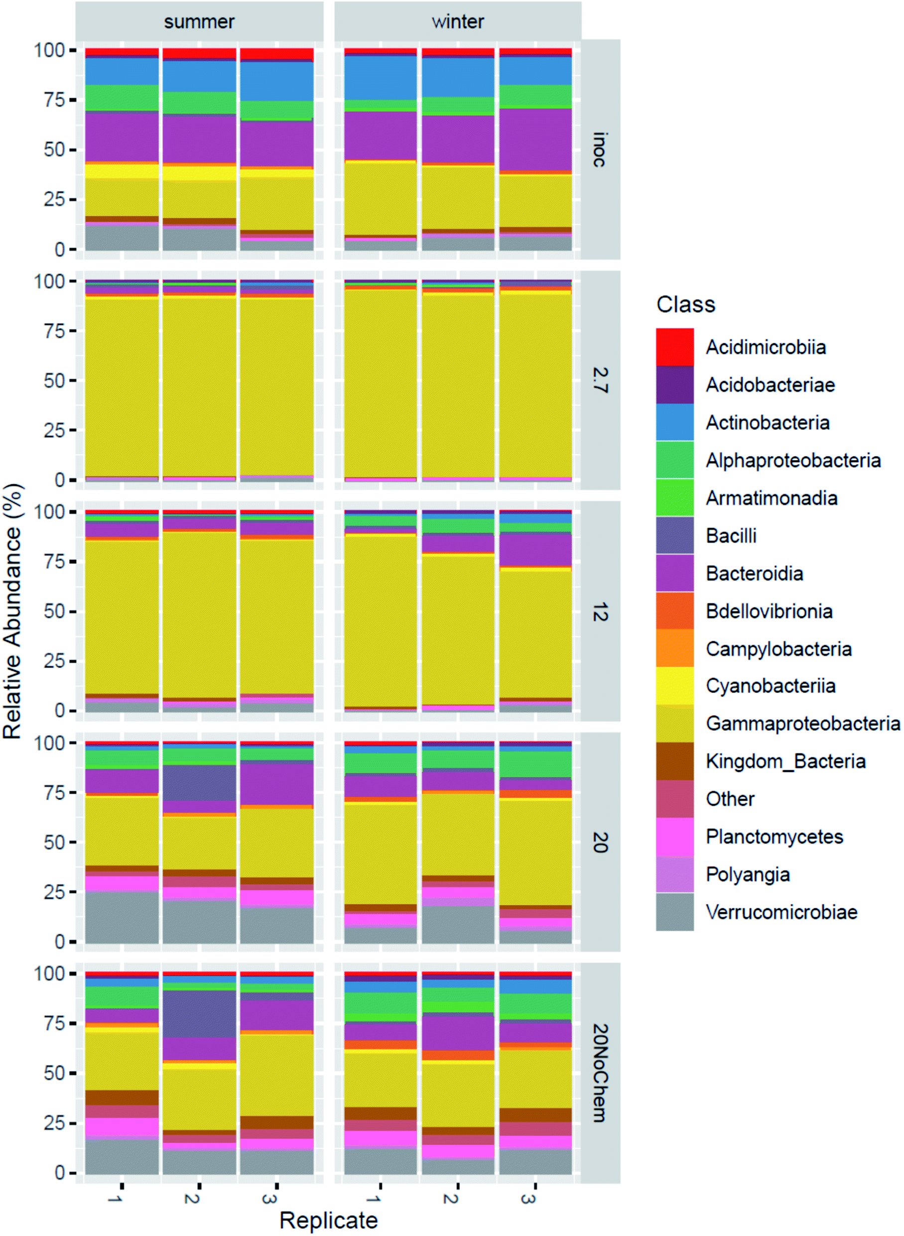 | ||
| Fig. 4 Microbial composition in the original inoculum from winter and summer and after 15 days incubation under four different treatments. | ||
The community composition of both inocula changed markedly during the 14 days incubations for all tested treatments (Fig. 3). The test temperature had a very clear and consistent effect on these changes. A permutational multivariate analysis of variance confirmed the significant effects of the test temperature, the inoculum and their interactions (p < 0.01) on microbial community composition. The adjusted R2 indicated that incubation temperature had a larger influence on the microbial community composition than inoculum origin (0.35 vs. 0.1).
Effect of test temperature on microbial community composition (spiked systems)
A large change in composition occurred during incubation at 2.7 and 12 °C for both inocula (Fig. 4), which seems to be linked to growth. This is evident from the qPCR analysis (ESI13 and ESI14†) where 16S rRNA gene copy numbers increased by 1.5 log units during the 15 days of incubation at these temperatures. The significant decrease in alpha diversity observed at 2.7 °C (Faith's phylogenetic diversity, p = 0.02 ESI13 and ESI14†), suggests that a limited number of bacterial types were responsible for this growth. Indeed, the 2.7 °C and 12 °C samples became dominated by gammaproteobacterial sequence variants that were not detected or close to detection limit in the inocula (ESI15†). The four most abundant sequence variants after incubation (two classified as Acinetobacter and two unclassified Comamonadacae), collectively accounting for 14–60% of the sequences, were undetected in the summer inoculum and only very marginally present in the winter one (average of 0.06% for the only two detected ASVs). This more than 2 log increase in relative abundance demonstrates the large growth that occurred in the two-week incubation, even at low temperature. At these temperatures, and especially at 2.7 °C, only little hydrocarbon biodegradation was detected at day 15 (ESI4†), suggesting that the observed growth was not primarily caused by hydrocarbon consumption. We hypothesize that the primary carbon and energy source at that point may have been the natural organic matter initially present in the freshwater inocula and that the sequence variants that proliferated might be the ones best adapted to grow on this substrate at low temperature.At day 15, the composition in the 20 °C incubations with chemicals was not dominated by the same sequence variants as in the two lower incubation temperatures (ESI15†). In fact, the four dominant ASVs at 2.7 and 12 °C were small contributors to the communities of the 20 °C samples (1–4%), and there was less evidence of growth in the qPCR data. We speculate that, at this higher temperature, growth on natural organic matter might have peaked before the day 15 sampling point and that bacterial density had subsequently decreased, due to predation and/or decay. This would be consistent with reports of microbial dynamics in similar assays where, in absence of spiked chemical, growth of an incubated fresh water sample peaked the first day of incubation at 20 °C and fell close to detection limit by day 10.16 A role of predation is supported by the observation of 46 ASV belonging to the bacterivorous class Bdellovibrio, collectively representing ∼3% in the 20 °C incubations (winter), increasing from <0.2% in the inoculum. Predation has been reported to have a significant effect on degradation of hydrocarbons in at least some situations.28 For the summer samples, there was no evidence of proliferation of Bdellovibrio, but we speculate that eukaryotic predators, undetectable with 16S rRNA gene analysis, such as protozoa, might have contributed to limiting prokaryotic density.
Effect of low concentration hydrocarbon mixture on microbial community composition
The samples incubated at 20 °C with and without chemicals have a similar overall composition (Fig. 3), indicating that the effects of the test chemicals on the microbial composition were limited compared to those caused by the different incubation temperatures discussed in the previous paragraph. However, differential count analysis revealed that the relative abundance of 228 ASVs were affected by the presence of the hydrocarbons. Many ASVs (148) were detected as more abundant in the presence of chemicals compared to absence of chemicals. It is likely that they include hydrocarbon degraders, especially since the qPCR data (ESI13 and ESI14†) suggests growth- or rather less decline in the 20 °C sample incubated with chemicals compared to the one without chemicals. This is consistent with the fact that the majority of the test chemicals were more than 50% degraded at day 15 at 20 °C. In particular, two genera appeared to have experienced growth exclusively in samples where hydrocarbon degradation occurred: Nevskia and Sulfuritalea. Nevskia was mostly present at 20 °C and Sulfuritalea at 12 and 20 °C, while neither were detected at 2.7 °C (ESI16 and ESI17†). Both genera have previously been associated with petroleum hydrocarbon degradation.29–31Conclusions
These dedicated experiments to link biodegradation kinetics, microbial composition and test temperature revealed a number of important observations for biodegradation testing and future development of standards biodegradation test methods.The obtained results confirmed the recent observation that the Arrhenius equation is describing the test-temperature dependency of petroleum hydrocarbon degradation well, when testing at the standard temperatures of 12 and 20 °C. Correction of biodegradation kinetics between these two test temperatures for an inoculum is thus warranted.
On the contrary, using inoculum adapted to summer temperatures in a test at very low temperature resulted in lack of biodegradation, even though biodegradation was seen in the winter inoculum incubated at the same low temperature. This observation stresses the importance of seasonal adaptation of the microbial community in the environment. Tests conducted at very low test temperatures should therefore apply inoculum sampled at temperatures close to the test temperature in order to improve environmental realism in the test. The observation also points to the need for more research on the effect of storage conditions for the inoculum prior to biodegradation testing, since cooling a warm adapted inoculum under storage might hamper the subsequent biodegradation.
The microbial community composition in the winter and summer inoculum were remarkably similar. The composition clearly changed during incubation for all treatments relative to the inoculum. This demonstrates that the decoupling of the inoculum from the environment and its incubation under constant test conditions strongly affected the microbial composition. The test temperature had a clear effect on the development of the microbial composition, which was consistent for both summer and winter inoculum. Overall, the decoupling from the environment and the conditions in the test seemed to affect the microbial composition more than the inoculum season, which asks for further research and possibly also for test method improvements.
The samples incubated with and without chemicals had a similar overall microbial composition, indicating that the effects of the test mixture on the microbial composition was limited at the low test concentrations of the present study. However, differential count analysis still revealed an effect of the presence of hydrocarbons. In particular, two genera, previously associated with petroleum hydrocarbon degradation, appeared to have experienced growth exclusively in samples where hydrocarbon degradation occurred, Nevskia and Sulfuritalea.
Funding sources
This study was funded by Concawe.Conflicts of interest
The authors state that there are no conflicts to declare.Acknowledgements
We are grateful to Hanne Bøggild, Susanne Kruse and Lene Kirstejn Jensen for technical assistance in the laboratory, and to the Concawe EMG group for their comments on the draft manuscript.References
- ECHA, Chapter R.11: PBT/vPvB Assessment, 2017 Search PubMed.
- R. Boethling, K. Fenner, P. Howard, G. Klečka, T. Madsen, J. R. Snape and M. J. Whelan, Integr. Environ. Assess. Manage., 2009, 5, 539–556 CrossRef CAS PubMed
.
- A. Kowalczyk, T. J. Martin, O. R. Price, J. R. Snape, R. A. van Egmond, C. J. Finnegan, H. Schäfer, R. J. Davenport and G. D. Bending, Ecotoxicol. Environ. Saf., 2015, 111, 9–22 CrossRef CAS PubMed
- H. Birch, H. R. Andersen, M. Comber and P. Mayer, Chemosphere, 2017, 174, 716–721 CrossRef CAS PubMed
- H. Birch, R. Hammershøj and P. Mayer, Environ. Sci. Technol., 2018, 52, 2143–2151 CrossRef CAS PubMed
- P. Shrestha, B. Meisterjahn, M. Klein, P. Mayer, H. Birch, C. B. Hughes and D. Hennecke, Environ. Sci. Technol., 2019, 53, 20–28 CrossRef CAS PubMed
- D. Salvito, M. Fernandez, K. Jenner, D. Y. Lyon, J. de Knecht, P. Mayer, M. MacLeod, K. Eisenreich, P. Leonards, R. Cesnaitis, M. León-Paumen, M. Embry and S. E. Déglin, Environ. Toxicol. Chem., 2020, 39, 2097–2108 CrossRef CAS PubMed
- P. N. H. Wassenaar and E. M. J. Verbruggen, Chemosphere, 2021, 276, 130113 CrossRef CAS PubMed
- G. Thouand, M. J. Durand, A. Maul, C. Gancet and H. Blok, Front. Microbiol., 2011, 2, 1–6 Search PubMed
- K. Fenner, M. Elsner, T. Lueders, M. S. Mclachlan, L. P. Wackett, M. Zimmermann and J. E. Drewes, ACS ES&T Water, 2021, 1, 1541–1554 Search PubMed
- D. Ribicic, K. M. McFarlin, R. Netzer, O. G. Brakstad, A. Winkler, M. Throne-Holst and T. R. Størseth, BMC Microbiol., 2018, 18, 1–15 CrossRef PubMed
- M. Posselt, J. Mechelke, C. Rutere, C. Coll, A. Jaeger, M. Raza, K. Meinikmann, S. Krause, A. Sobek, J. Lewandowski, M. A. Horn, J. Hollender and J. P. Benskin, Environ. Sci. Technol., 2020, 54, 5467–5479 CrossRef CAS PubMed
-
Organisation for Economic Co-operation and Development, OECD 309: Aerobic Mineralisation in Surface Water – Simulation Biodegradation, 2004 Search PubMed
- H. Birch, R. Hammershøj, M. Comber and P. Mayer, Chemosphere, 2017, 184, 400–407 CrossRef CAS PubMed
- R. Hammershøj, H. Birch, A. D. Redman and P. Mayer, Environ. Sci. Technol., 2019, 53, 3087–3094 CrossRef PubMed
- R. Hammershøj, K. K. Sjøholm, H. Birch, K. K. Brandt and P. Mayer, Environ. Sci.: Processes Impacts, 2020, 22, 2172–2180 RSC
-
ECHA, Guidance on Information Requirements and Chemical Safety Assessment Chapter R.16: Environmental Exposure Assessment Version 3.0 February 2016, Helsinki, European Chemicals Agency., 2017 Search PubMed
- K. K. Sjøholm, H. Birch, R. Hammershøj, D. M. V. Saunders, A. Dechesne, A. P. Loibner and P. Mayer, Environ. Sci. Technol., 2021, 55, 11091–11101 CrossRef PubMed
- M. Honti, F. Bischoff, A. Moser, C. Stamm, S. Baranya and K. Fenner, Water Resour. Res., 2018, 54, 9207–9223 CrossRef
- R. V. Southwell, S. L. Hilton, J. M. Pearson, L. H. Hand and G. D. Bending, Sci. Total Environ., 2020, 733, 139070 CrossRef CAS PubMed
- R. Hammershøj, H. Birch, K. K. Sjøholm and P. Mayer, Environ. Sci. Technol., 2020, 54, 4974–4983 CrossRef PubMed
- Aarhus University, Overfladedatabasen ODA, https://odaforalle.au.dk/, accessed 10 February 2021.
- K. E. C. Smith, N. Dom, R. Blust and P. Mayer, Aquat. Toxicol., 2010, 98, 15–24 CrossRef CAS PubMed
-
R. P. Schwarzenbach, P. M. Gschwend and D. M. Imboden, Environmental Organic Chemistry, John Wiley & Sons, New Jersey, US, 2nd edn, 2003 Search PubMed
- S. Simkins and M. Alexander, Appl. Environ. Microbiol., 1984, 47, 1299–1306 CrossRef CAS PubMed
- A. Apprill, S. Mcnally, R. Parsons and L. Weber, Aquat. Microb. Ecol., 2015, 75, 129–137 CrossRef
-
ECHA, Guidance on Information Requirements and Chemical Safety Assessment Chapter R.7b: Endpoint Specific Guidance, 2017, vol. 2012 Search PubMed
- S. Otto, H. Harms and L. Y. Wick, FEMS Microbiol. Ecol., 2017, 93, 1–7 CrossRef CAS PubMed
- B. Wang, Y. Teng, Y. Xu, W. Chen, W. Ren, Y. Li, P. Christie and Y. Luo, Sci. Total Environ., 2018, 640–641, 9–17 CrossRef CAS PubMed
- T. Fang, H. Wang, Y. Huang, H. Zhou and P. Dong, Int. J. Syst. Evol. Microbiol., 2015, 65, 1666–1671 CrossRef CAS PubMed
- E. Kim, A. Yulisa, S. Kim and S. Hwang, Bioresour. Technol., 2020, 306, 123178 CrossRef CAS PubMed
Footnote |
| † Electronic supplementary information (ESI) available. See DOI: 10.1039/d1em00319d |
| This journal is © The Royal Society of Chemistry 2022 |