Quantitative spatiotemporal mapping of thermal runaway propagation rates in lithium-ion cells using cross-correlated Gabor filtering

Abstract

Abuse testing of lithium-ion batteries is widely performed in order to develop new safety standards and strategies. However, testing methodologies are not standardised across the research community, especially with failure mechanisms being inherently difficult to reproduce. High-speed X-ray radiography is proven to be a valuable tool to capture events occurring during cell failure, but the observations made remain largely qualitative. We have therefore developed a robust image processing toolbox that can quantify, for the first time, the rate of propagation of battery failure mechanisms revealed by high-speed X-ray radiography. Using Gabor filter, the toolbox selectively tracks the electrode structure at the onset of failure. This facilitated the estimation of the displacement of electrodes undergoing abuse via nail penetration, and also the tracking of objects, such as the nail, as it propagates through a cell. Further, by cross-correlating the Gabor signals, we have produced practical, illustrative spatiotemporal maps of the failure events. From these, we can quantify the propagation rates of electrode displacement prior to the onset of thermal runaway. The highest recorded acceleration (≈514 mm s⁻²) was when a nail penetrated a cell radially (perpendicular to the electrodes) as opposed to axially (parallel to the electrodes). The initiation of thermal runaway was also resolved in combination with electrode displacement, which occurred at a lower acceleration (≈108 mm s⁻²). Our assistive toolbox can also be used to study other types of failure mechanisms, extracting otherwise unattainable kinetic data. Ultimately, this tool can be used to not only validate existing theoretical mechanical models, but also standardise battery failure testing procedures.

---

Introduction

Lithium-ion batteries offer a convenient power source for a broad range of mobile technologies,¹ as well as the potential to reduce greenhouse gas emissions, particularly in transport applications, if their life cycle is managed sustainably.² They are also finding increasing use in residential and grid energy storage.³ However, their growing uptake poses a safety issue, owing to the potential for highly energetic failure events to occur. These can be triggered in a number of ways, such as electrically (short-circuiting),⁴ thermally (overheating),⁵ or mechanically (impact or penetration),⁶ and can ultimately lead to explosions, fires, and the release of toxic and flammable ejecta and gases.^3,7 Although catastrophic failure is uncommon, occurring in around 1 in 10 million units,¹ tens of billions of batteries enter the market each year, making the risk significant.⁸ This is a particular concern for ‘mission critical’ applications, for example in communications, electric vehicles and aerospace, in which the integration of lithium-ion batteries is hampered by concerns with their safety and reliability.⁹ Therefore, to enable their continued uptake, it is crucial that lithium-ion battery failure is better understood, such that safer batteries may be engineered, with improved solutions and mitigation strategies for failure.

X-ray radiography is a powerful tool for capturing the degradation of individual lithium-ion cells operando, under both standard operation and abuse testing conditions.^4,5,10–12 Real-time and high-speed (i.e., slow-motion) imaging offer a valuable insight into the mechanisms of failure, through directly observable changes to the cell structure. X-ray radiography can track three-dimensional structural information at high speeds (i.e., 2000 Hz) offering unparalleled insights into battery failure. Additionally, the efficacy of hazard mitigation strategies, such as safety vents, separator shutdown and current interruption, and positive temperature coefficient devices, may also be investigated.⁴ However, most failure/safety testing methods do not have accompanying high-speed X-ray radiography data, and the analysis and interpretation of any such available data has remained largely qualitative. This is due to the presence of multiple complex events, involving both gradual and sudden shifts of the electrodes, and their decomposition, as well as, in some cases, the movement of a large object such as a nail. This poses a significant image-processing challenge, for which there is currently no robust, quantitative analytical approach. Typically, videos are examined by eye, with frames of interest selected to produce a timeline of visible events. Although informative, this is a very slow method, owing to the large amounts of information present in a single video, and mechanisms are typically postulated from qualitative observations. By extension, a broad, statistically significant analysis of multiple videos using the same approach is not only extremely time-consuming, but also supremely challenging. Subtle yet key events may also not be apparent to the eye, and such manual observations are likely to be inconsistent between measurements (due to the stochastic nature of these failure events) and between researchers undertaking the data analysis.¹³ A robust analytical toolbox for quantifying the kinetics of cell failure is therefore required in order to fully exploit the information contained with existing and future X-ray radiography data that are now being collated in open-access databases (e.g., the Battery Failure Databank hosted by the National Renewable Energy Laboratory¹⁴).

The internal structure of a lithium-ion cell is typically an assembly of periodic electrode layers, current collectors and separators. In X-ray radiography, this produces a distinct image ‘texture’, composed of bands of compositional contrast resulting from the different X-ray attenuation coefficients of each material. While a variety of feature-detection and object-classification algorithms are available, X-ray radiography of lithium-ion cell failure poses a unique combination of challenges that hinder their applicability:

(i) Although the electrode texture is well-defined, it degrades unevenly across the field of view, disappearing as failure occurs. Frequency-domain analyses, such as fast Fourier transforms, that can identify the initial texture based on spatial or temporal frequencies,¹⁵ are unable to track the changes in phase and orientation in the spatial domain as failure progresses.

(ii) High frequency noise is typically present, making the identification of periodic or aperiodic features challenging. Pixel-based region-labelling algorithms fail in accurately deconvoluting the noise from the features of interest.

(iii) In some cases, for example during nail penetration testing, large objects are present in the field of view. These obscure objects introduce variations in the texture, leading to analytical artefacts.

In this work, we apply Gabor filter banks and subsequent post-processing algorithms to high-speed X-ray radiography data of lithium-ion cells undergoing abuse via nail penetration and ball compression testing. Gabor filter banks are commonly used in visual processing, owing to their sensitivity to the orientation (angle) and spacing (frequency) of edge features.^16,17 They have been effective in the automated recognition of textures,^18,19 structural variations in electron microscopy images,^20–23 anatomical structures in X-ray computed tomograms,^24,25 as well as human faces²⁶ and fingerprints.²⁷ Texture may be detected and quantified as a function of component feature size, orientation and distribution. The ability to control the frequency and orientation of the Gabor filters enables the user to selectively pick out the electrode texture and omit other objects. Furthermore, the filters can track changes in the spatial domain (directional sensitivity) as failure progresses within a cell. Ultimately, this approach produces frequency-sensitive spatial information, while at the same time being noise-insensitive. Thus, it addresses the challenges outlined above and is a powerful and an appropriate technique for analysis of X-ray radiography data.

We have developed an image processing toolbox outlined in the following manner:

(i) We firstly objectively identify the internal cell structure and nail as separate textures, representing them as Gabor-filtered frames with features defined by distinct functions of angle and frequency. While failure may be induced in any direction, the electrodes present a highly ordered structure that can be resolved based on its particular orientation.

(ii) The Gabor-filtered frames are then cross-correlated over time, facilitating the tracking of the degradation and failure of cells with a high spatiotemporal resolution and allowing us to estimate the displacement of electrode layers before failure.

(iii) Finally, from the conversion to spatiotemporal information we produce a single practical, and illustrative map of the failure events occurring in an entire video, from which we quantify the rate of propagation of failure both axially (parallel to the electrodes) and radially (perpendicular to the electrodes).

Battery failure involves multiple complex events occurring in all three dimensions. Using our technique, we have, for the first time, tracked how the structure of electrodes changes over time, as a direct result of the forces acting on it. Not only does our approach introduce a means of quantifying failure processes, but it may also facilitate the validation of existing mechanistic models. Our spatiotemporal maps reveal that the rate of electrode displacement (before the onset of failure) is higher when a nail propagates radially rather than axially. We also identify and track the onset of failure, which occurs at slower velocities than the electrode displacement and exhibits varied third-order kinetic behaviour. With the spatiotemporal maps, we may accurately describe not only ‘where and when’ failure originates, but also ‘how’ it propagates over time. In the long term, we are confident that this toolbox can further the understanding of battery degradation mechanisms by coupling mechanical failure models^28–30 with electrochemical thermal-runaway models.³¹ Furthermore, our approach provides an open-source analytical toolbox developed on Python that may be readily implemented on video data from any instrumental setup, including legacy data from archives (toolbox available upon request). Furthermore, the toolbox has a user-friendly interface to guide appropriate parameter selection. Not limited to visual assessments, any user may thus gain new perspectives on their data, from which they may readily distinguish interesting behaviours for further characterisation. Analysing a variety of datasets, each of which were clearly distinct from one another in both input and output, we have evidenced that our technique is an extremely robust, efficient, informative and transferable means of analysing such dense datasets. Our technique is therefore extremely promising in advancing and strengthening the understanding of failure mechanisms of lithium-ion cells.

Experimental

Failure testing setup

The nail penetration testing was performed as previously described by Finegan et al. (2017)⁶ inside a commercial nail penetration system (MTI Nail Penetration Tester, MSK-800-TE9002, MTI, Richmond, CA, USA), modified to have X-ray transparent 2 mm thick aluminium front and rear panels for X-ray imaging. The lithium-ion cells were held in place by hydraulic clamps that operated at 4 bar. The hydraulic piston nail penetrator was connected to a 5 bar air supply. All tests were carried out using the smart nail described by Finegan et al. (2017)⁶ or a stainless steel ball of diameter 20 mm (see Table 1). Briefly, the smart nail is a 60 mm long stainless steel tube with an external diameter of 4 mm and an internal diameter of 2 mm.³² The nail contains a thermocouple and has a conical tip that was sharpened using a lathe.

Table 1 The analytical toolbox was tested on four datasets that involved failure testing using mechanical objects incident with the cells at different locations and orientations

Dataset name	Test type	Cell type	Incidence angle of object (with respect to the central axis of the electrode structure)	Location of test (along the length of the cell)
SI_Video_1.mp4	Nail penetration	LG ICR18650S3	Perpendicular	Middle
SI_Video_2.mp4	Nail penetration	LG ICR18650S3	Perpendicular	Middle
SI_Video_3.mp4	Nail penetration	LG ICR18650S3	Parallel	Bottom
SI_Video_4.mp4	Ball compression	LG ICR18650B4	Perpendicular	Middle

---

Collection of X-ray radiography data

X-ray radiography was carried out at beamline ID19 at the European Synchrotron Radiation Facility (ESRF). A polychromatic beam was used with a LuAG:Ce (Lu₃Al₅O₁₂:Ce) scintillator and a high-speed PCO.Dimax camera (PCO AG, Germany). Images were captured at 2000 fps with an exposure time of 457 μs and 10 μm pixel-size. The raw data were processed where flat-field correction was applied using a bespoke MATLAB code. The resulting videos are provided as Videos (‘SI_Video_1’–‘SI_Video_4’, ESI†).

Processing of radiography data

The pre-processed radiography data were opened in a bespoke analytical toolbox developed on Python 3,³³ with the following packages installed: imageio,³⁴ numpy,³⁵ scipy,³⁶ scikit-image,³⁷ matplotlib,³⁸ and tkinter.³⁹ An experimental dataset consisting of a single AVI/MP4 video or Tiff stack, or a folder of images, was loaded through the imageio package and presented on a graphical interface via tkinter, where the user can select the region of interest (ROI) and the set of frames to be analysed. For datasets, especially legacy data that have gone through video compression software, where the number of frames has been altered – either through the introduction of duplicate frames or dropped frames, the original frame rate of video capture cannot be used for temporal analysis. To this end, the original timestamp embedded in the frames can be analysed using Google's optical character recognition engine, Tesseract,⁴⁰via Pytesseract,⁴¹ a wrapper for Python. Any duplicate frames were ignored from analysis based on the detected timestamps.

For a set of frames loaded, we define t = 0 s as the first frame selected for analysis, unless otherwise stated, for which the electrode structure is assumed to be pristine and unaffected by any abuse process. t_i is defined as the time of the ith frame, where i frames are included in the analysis. All spatial information has been presented in the Cartesian coordinate system, where x represents the position in the axial direction, along the X axis (parallel to the electrodes), and y represents the position in the radial direction, along the Y axis (perpendicular to the electrodes). Unless otherwise stated, the origin, x = 0 mm, y = 0 mm, is the top-left corner of the rectangular ROI selected by the user.

Upon converting the frames to an 8-bit greyscale format, the contrast range of each selected frame was normalised (lowest pixel value set to 0 and highest pixel value set to 255) and a morphological reconstruction step applied to smoothen noise.⁴² Gabor filter banks were then applied as discrete sinusoidal waves modulated by a Gaussian function. This implementation consisted of a [9 × 9] pixel kernel, which scans across a frame (Fig. 1). The user can choose the most appropriate Gabor filter parameters (angle and frequency), which are then applied on all the selected frames of a dataset.

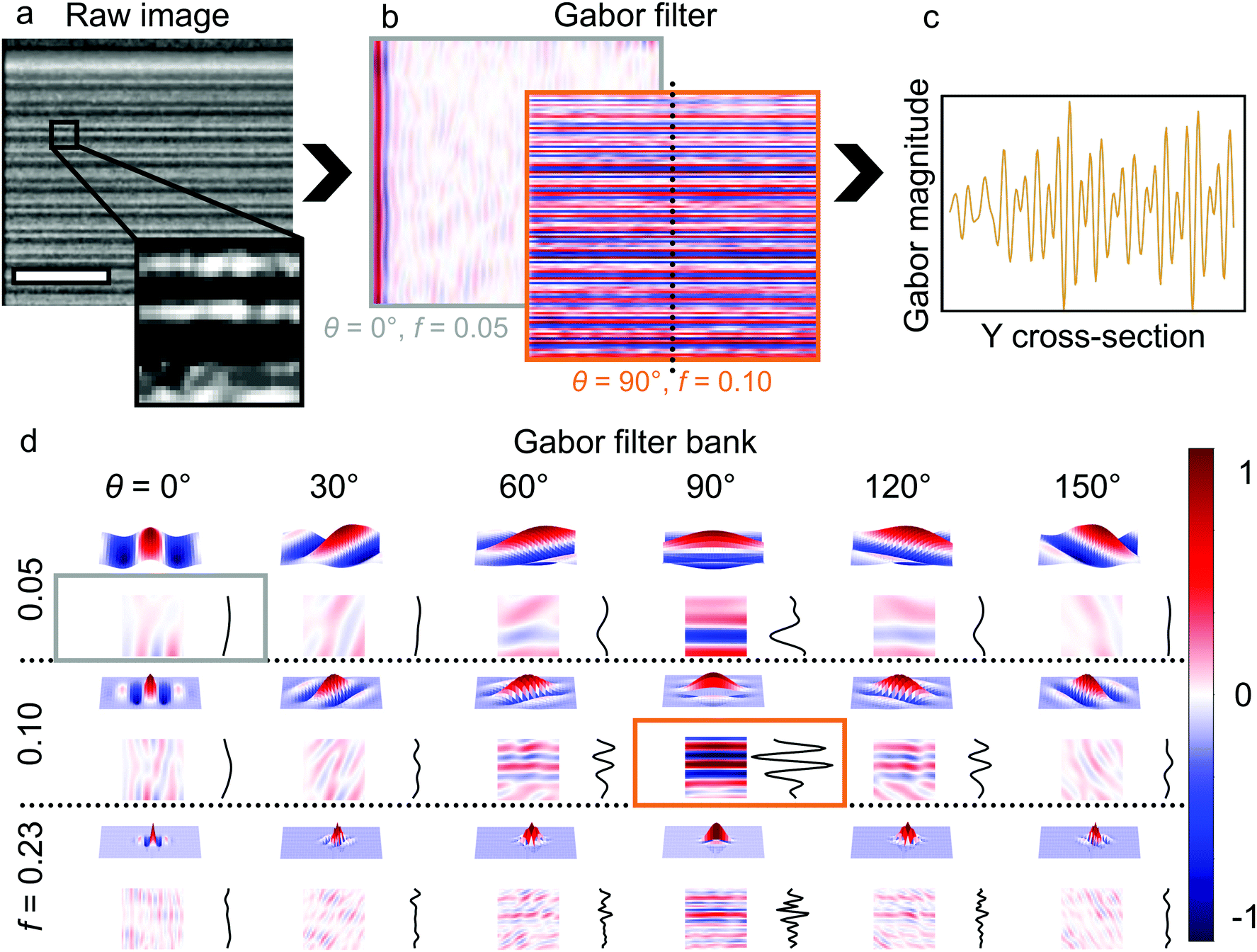Fig. 1 Directional texture classification using the Gabor filter. (a) A typical X-ray radiography frame captured at 2000 fps showing the electrode layers. The scale bar indicates 1 mm. (b) Images filtered using the Gabor kernel as shown in (d); the electrodes are filtered out when the filter (the sinusoidal harmonic function) is applied perpendicular to the electrodes (radially, θ = 0°), whereas the electrode structure is captured when filter is applied parallel to the electrode layers (axially, θ = 90°). (c) Y cross-section of the image filtered at θ = 90°, representing the output of the Gabor filter that is most sensitive to the structure of the electrodes. (d) Gabor kernels with a sinusoidal wavelet (3D projections) applied at varying angles (θ) and frequencies (f) on the inset image shown in (a). θ offers directional sensitivity to selectively filter ‘texture’ of the electrodes and the frequency (f) resolves the individual electrode layers (optimal at f = 0.10 pixels⁻¹). The output signal is maximised for θ = 90° and f = 0.1, i.e., for the filter which best matches the orientation and spacing of the electrodes (orange inset). For filters that do not match with the electrodes, the output signal is reduced, and the texture is not well-represented (grey inset). For an appropriately filtered image, a Gabor signal of +1 represents the Cu/Al layers, −1 that of graphite/electrolyte and values around 0 represent the separator material or the Cu-anode interface/Al-cathode interface.

Following the Gabor filtering step as shown in Fig. 1, post-processing analyses were performed on the filtered frames (Fig. 1c), to estimate electrode displacements and build temporal and spatiotemporal maps, enabling the extraction of cell failure kinetics.

Results and discussion

The cell types, the failure-testing modes, and the location of the tests are shown in Table 1. ‘SI_Video_1’ and ‘SI_Video_2’ (ESI†) involve radial penetration of the smart nail midway along the cell. ‘SI_Video_3’ (ESI†) entails axial propagation of the nail, where the nail penetrates through the base of the cell. ‘SI_Video_4’ (ESI†) involves compression of the electrodes by a ball, incident midway along the cell.

Texture detection using Gabor filters

We firstly applied a Gabor filter bank to a video to determine the efficacy of capturing the texture in each frame, representing the electrodes. Fig. 1a shows an example video frame, for which a pair of Gabor-filtered output images are shown in Fig. 1b. In the foreground image, which has been filtered optimally (filter applied parallel to the electrodes, with a frequency similar to the electrode spacing), the electrode structure shows up as a strong signal (red – positive peak representing Cu/Al, blue – negative peaks denoting electrolyte or the graphite layer, and whites that represent the separator material or the Cu-anode/Al-cathode interface). On the other hand, in the background image, which has been filtered poorly (filter applied perpendicular to the electrodes, with a low frequency), there are no features detected, aside from an artefact at the left side of the image. Taking a Y cross-section through the optimally filtered data, as shown in Fig. 1c, produces a very clear representation of the alternating electrode structure. So, by using an appropriate choice of filtering conditions (orientation, θ and frequency, f, for example from those shown in Fig. 1d), we acquire output data which do not contain the high-frequency noise present in the raw image, with an electrode spacing and relative contrast that are extremely well-defined between large positive and negative values (normalised here, and in the rest of the manuscript, to ±1).

Once we had chosen optimal Gabor filter parameters for a single frame of ‘SI_Video_1’ (ESI†), we applied the same process to each frame in the dataset and extracted the resulting cross-sections for comparison. This allowed us to monitor the condition of the cell over time. Fig. 2a, d and g show raw video frames of a nail gradually penetrating a cell and disrupting the electrodes. To the eye, there is a clear distinction between the nail and the electrodes, but to precisely define their relative arrangement is not trivial, particularly as the nail moves further into the cell and the electrodes deform. However, by filtering the images at θ = 0° (radially) and θ = 90° (axially), we were able to selectively identify the electrodes independently and filter out the nail. Fig. 2b, e, and h show the output frames filtered parallel to the nail. The signal is initially just noisy throughout the cell, i.e., the electrode texture is not picked out by the filter. When the nail enters, we observe the appearance of a corresponding texture perpendicular to the electrodes. Conversely, when the filter is aligned with the electrodes, as in Fig. 2c, f, and i, the signal is initially very pronounced. Its magnitude then decreases in accordance with the texture changing as the nail enters and causes a region of deformation to spread from its entry point (see ‘SI_Video_5.avi’ (ESI†) for an animated comparison of the Gabor filter ranging from θ = 0° to 180°). The outcomes of these contrasting outputs of the filters are highlighted in the bottom row of Fig. 2, which shows single-pixel-wide Y cross-sections from the centres of the filtered images. So, the Gabor signal cross-sections allow us to compare distinct features by tracking, over time, the textures that best describe them. As the texture changes, such as the electrodes losing structural integrity, the corresponding signal changes.

Fig. 2 Selective Gabor kernel filtering of electrode ‘texture’ from the dataset ‘SI_Video_1’ (ESI†). The top row shows video frames at different times during nail penetration. The second row shows the results of applying the Gabor filter at θ = 0° to the video frames. The inner core of the smart nail is detected, while the electrodes are not. The third row shows the results of applying the filter at θ = 90° to the video frames. Here, the electrode texture is captured. However, as the nail penetrates the electrodes, it is filtered out because the texture is no longer aligned with the filter. Plots in the bottom row show the normalised Gabor signals of the electrode structure at θ = 90° (black lines) and θ = 0° (orange lines). As electrodes deform due to the nail (time = 0.437 s), the Gabor signal decreases accordingly due to reducing alignment of image features with the applied filter. The electrode signal in the central region of frame, at time = 0.51 s, has disappeared as the electrodes have been entirely displaced by the nail. A Gabor map of the nail and the electrode layers in frame, at time = 0.437 s, filtered from θ = 0° to 180° has been shown in the Video ‘SI_Video_5.avi’ (ESI†). The scale bar indicates 4 mm.

Tracking the nail velocity

To expand the functionality of our Gabor filtering approach, we quantified the nail velocity using the video frames between t = 0.2075 s and t = 0.5445 s from ‘SI_Video_1’ (ESI†) (where t = 0 s refers to the first frame of analysis of the dataset shown in Fig. 2a). Fig. 3a shows a raw video frame, with the ROI cropped for nail tracking shown in Fig. 3a-(i). The corresponding Gabor-filtered frame is shown in Fig. 3a-(ii), where filter parameters of θ = 140° and f = 0.04 pixels⁻¹ have been used in order to align the filter with the edge of the conical tip of the nail. The nail's conical tip is clearly highlighted by the filter, isolated from the rest of the ROI, and appears as a distinctive peak in the Y cross-section, as shown in Fig. 3b (blue circle marker) at a given frame. Applying the filter to each cropped video frame and finding the position of this peak (black markers) allowed us to calculate the displacement of the nail tip over time, as shown in Fig. 3c. Thus, we may follow its trajectory and determine its velocity (see Video ‘SI_Video_6.avi’, ESI†). The nail pierces the cell casing and moves with a rather constant velocity of around 2.22 mm s⁻¹, balanced by the mechanical resistance of the electrodes. The electrodes then tear suddenly (t ≈ 0.4645 s), allowing the nail to accelerate to a peak velocity of 113 mm s⁻¹ under continued application of its driving force. It is worth noting that this is the first instance in which quantification of such information characterising cell failure has been reported. The understanding of safety testing procedures may therefore be enhanced by applying our toolbox to a range of failure scenarios. Such insight is likely to lead to improved cell safety standards, and thus engineering solutions for the production of safer cells.

Fig. 3 Tracking the velocity of a nail puncturing a cell. (a) A video frame was cropped around the nail (i) and a filter at θ = 140° and f = 0.04 pixels⁻¹ applied (ii), to select one-half of the conical tip of the nail in the dataset ‘SI_Video_1’ (ESI†). (b) Y cross-section of the normalised Gabor signal from (a) (ii), where the peak represents the position of the edge of the nail. The blue circle marker denotes the peak at the current frame, whereas the small black circle markers denote the peak positions in the preceding frames (i.e., the path taken by the nail edge from t = 0.2075 s). (c) Displacement profile of the nail determined from the relative positions of the tip-edge peak. The vertical dotted line denotes the timestamp of the frame shown in (a and b). A temporal map of the nail and its displacement determination are available in the Video ‘SI_Video_6.avi’ (ESI†). A peak nail velocity of 113 mm s⁻¹ was estimated at t = 0.4645 s, i.e., the point when the electrodes fractured and the nail accelerated, leading to the steepest change in displacement. The scale bar indicates 4 mm.

Temporal cross-correlation of the Gabor signal

To quantify changes to the cell structure over time, we tracked the Gabor signal at a single X cross-section over time, as shown in the top plot of Fig. 4a. This location was chosen from the dataset shown in Fig. 2, close to the surface of the nail (x ≈ 4.7 mm). Fig. 4a shows how the electrode structure in close proximity to the nail shifts over time before finally failing mechanically. We then compared the signal at time t_i to the initial signal at time t₀ using cross-correlation, i.e., we calculated the similarity between the initial signal and signals from each subsequent frame. This is shown in the bottom plot of Fig. 4a, wherein the radial information (Y cross-section) at the chosen X cross-section in each frame is collapsed into a single value representing the ‘similarity’ with the first frame. When the cross-correlation is large and positive, the texture at t_i resembles the initial texture at t₀ (Fig. 4b, t₁). When the value is large and negative, the signal appears inverted (Fig. 4b, t₃), i.e., the electrodes have shifted a distance equal to half the electrode thickness from its original position. When the value is close to zero, there is either a complete misalignment between the signals (Fig. 4b, t₂) or the Gabor signal is low at time t_i, corresponding to the absence of electrode texture in the images (Fig. 4b, t₄). Until around 0.47 s in Fig. 4a, we can see that the electrodes shift gradually and linearly due to the mechanical force from the nail. From the temporal cross-correlation, this corresponds to the electrodes moving out of alignment and then realigning with neighbouring layers, giving a total shift of around 1.5 electrode layers (i.e., 1.5 full ‘oscillations’ are present in the shifting signal). When, at t_i, the Gabor peak of an electrode layer aligns with the t₀ position of a neighbouring layer, the cross-correlation value is large and positive, corresponding to one complete ‘electrode shift’, seen as the second maxima in the cross-correlation plot. The temporal cross-correlation also accurately indicates the time at which the electrode structure completely failed (i.e., when the correlation becomes a flat line around zero) at t ≈ 0.461 s. Although these processes may be observed in the raw video, they are challenging to quantify by eye, especially when thousands of frames must be examined. Instead, our toolbox can direct the user to the time-point corresponding to the failure event, as well as quantify the preceding behaviour as a function of time.

Fig. 4 Temporal cross-correlation of the electrode texture from the dataset ‘SI_Video_1’ (ESI†). (a) Top plot – 2D map showing the temporal evolution of the normalised Gabor signal at a fixed X position, and bottom plot – corresponding normalised temporal cross-correlation, where the Gabor signals at time t_i is cross-correlated with that of time t₀ (undisturbed electrode structure). (b) Comparison of Gabor signals at different times, t_i (orange lines), with that of t₀ (black lines). When the electrode texture has a high similarity with the undisturbed texture (t₀), the correlation value is large and positive (normalised to +1), e.g., at t₁ where t₁ − t₀ = 5 ms. When the electrode is displaced and so appears inverted compared with the initial texture at t₀, the correlation is large and negative (normalised to −1), e.g., at t₃ where t₃ − t₀ = 126 ms. When there is little or no similarity between the textures at t_i and t₀, the correlation value is close or equal to zero. This happens in two scenarios – when the electrode texture is displaced slightly but not inverted (e.g., at t₂ where t₂ − t₀ = 43.5 ms) or when the electrodes are completely delaminated or expelled from the field-of-view (e.g., at t₄ where t₄ − t₀ = 620 ms).

Estimation of electrode displacement

We extended our temporal cross-correlation to multiple X positions, which enabled us to observe the displacement of the electrodes along the length of the cell over time. We initially tried to identify and track individual peaks in the Gabor signal, but this proved problematic due to the disorderly nature of the failure; as electrode layers degraded, their corresponding peaks were lost, while new peaks were introduced by the cell casing entering the ROI due to the force of the nail. These issues produced mismatches in the peak tracking, rendering such algorithms impractical.

Instead, we estimated the electrode displacement using the temporal cross-correlation. This methodology was developed using ‘SI_Video_4’ (ESI†) as an ideal test case, involving compression of the electrodes by a ball (see Table 1), without subsequent mechanical failure or thermal runaway. Fig. 5a shows the raw video frames at t₀ and t_i = 0.5 s, where the electrodes demonstrate a clear, symmetric shifting and bending under the incident ball. Fig. 5b shows three temporal cross-correlations at different X positions. At x₂, corresponding to the centre of the ball, more electrode shifts (full oscillations in the cross-correlation) are present in comparison to x₁ and x₃, at the edges of the ball. We estimated the electrode displacement by multiplying the number of shifts by the distance between electrodes, 66 ± 17 μm, which we calculated from the average distance between adjacent Gabor peaks in the ‘pristine’ structure, i.e., at t₀.

Fig. 5 Estimation of electrode displacement. (a) X-ray frames of a ball compressing the cell at t = 0 s (top) and 0.5 s (bottom) from dataset ‘SI_Video_4’ (ESI†). (b) The normalised temporal cross-correlation signals of the electrode structure at three positions, x₁, x₂, and x₃ (vertical dotted lines in (a)), where each positive peak indicates one complete shift of the electrodes into alignment with the initial position of their neighbouring electrode layer. At t = 0.5 s, the electrodes at x₂ have traversed 6.73 ‘electrode shifts’ from their original position. From the Gabor signal profiles at t = 0 s, the distance between electrode layers was estimated to be 66 ± 17 μm, so at t = 0.5 s, the electrode structure at x₂ is displaced by an estimated 444 ± 115 μm from its original position. (c) Electrode displacement at various X positions for the dataset ‘SI_Video_4’ (ESI†). (d) Electrode displacement at various X positions for the nail penetration dataset ‘SI_Video_1’ (ESI†), where the distance between electrode layers was estimated to be 111 ± 10 μm. Analysis was cropped at t = 0.6 s, when the electrode layers fractured. At x = 6.7 mm (near the surface of the nail), the electrode displacement is estimated to be 221 ± 21 μm, above which the Gabor signals were lost. Error bars denote ±1 standard deviation in the distance between electrode layers.

Fig. 5c, shows the resulting electrode displacement across the video frame at six time-points between t₀ and t_i = 0.5 s. Directly below the centre of the ball, the displacement was the greatest, around 0.44 mm at 0.5 s. This drops off symmetrically in both x directions, to a minimum of around 0.08 mm at a distance of around 3.5 mm from the centre of the ball. We also note, from the broader colour bands in the centre of the plot (around x = 3.5 mm), that the displacement had a larger acceleration directly below the ball. We applied a similar approach to the nail penetration dataset ‘SI_Video_1’ (ESI†). Fig. 5d shows the displacement of the electrodes, wherein the nail (radius = 2 mm) is incident at the right side of the ROI (x = 6.7 mm). Here, the entire structure shifts homogeneously by around 0.1 mm over 0.36 s, before the displacement at the nail location becomes much more pronounced, and then stops at around 0.22 mm, when the Gabor signals were lost. This is an interesting contrast with the ball compression, which instead produced a continuous bending. The initial homogenous shifting of the electrodes in the nail penetration dataset resulted from the overall displacement of the cell as the nail made contact, followed by displacement of the electrodes as the nail pierced through. We note that this is in the plastic flow regime, where the volumetric stress withstood by the electrodes is a property of their tensile strength and Poisson ratio, as discussed by Wierzbicki and Sahraei, 2013.⁴³ Subsequently, as discussed above, the mechanical resistance of the electrodes suddenly yields as their structure fractures, leading to an abrupt acceleration of the nail (to a maximum of 113 mm s⁻¹ as shown in Fig. 3c).

Constructing spatiotemporal failure maps

We expanded our analysis by mapping the evolution of the cell structure in the ROI for the whole video in order to visualise the entire failure on a single spatiotemporal map. Fig. 6 shows the progression from cross-correlation information to mapping, using the dataset ‘SI_Video_1’ (ESI†). Fig. 6a shows the temporal cross-correlation plots at four X positions. Separately, these do not provide information on the failure propagation in the axial direction. However, to overcome this, we may plot the cross-correlation at every X cross-section as a surface plot to yield a spatiotemporal map, as shown in Fig. 6b. Such a map may be directly compared to the raw video frames, with time passing (positive vertical direction) as events develop across the X axis, (which is aligned with the width of the frames analysed). It is important to note that representing the data in this way captures the y information at each t as a single cross-correlation value. Regions of high similarity to the initial electrode texture appear red, and regions of inverted alignment appear blue. Regions of complete misalignment or disappearance of the texture from the ROI are intermediate and appear green. The map may then be interpreted as follows: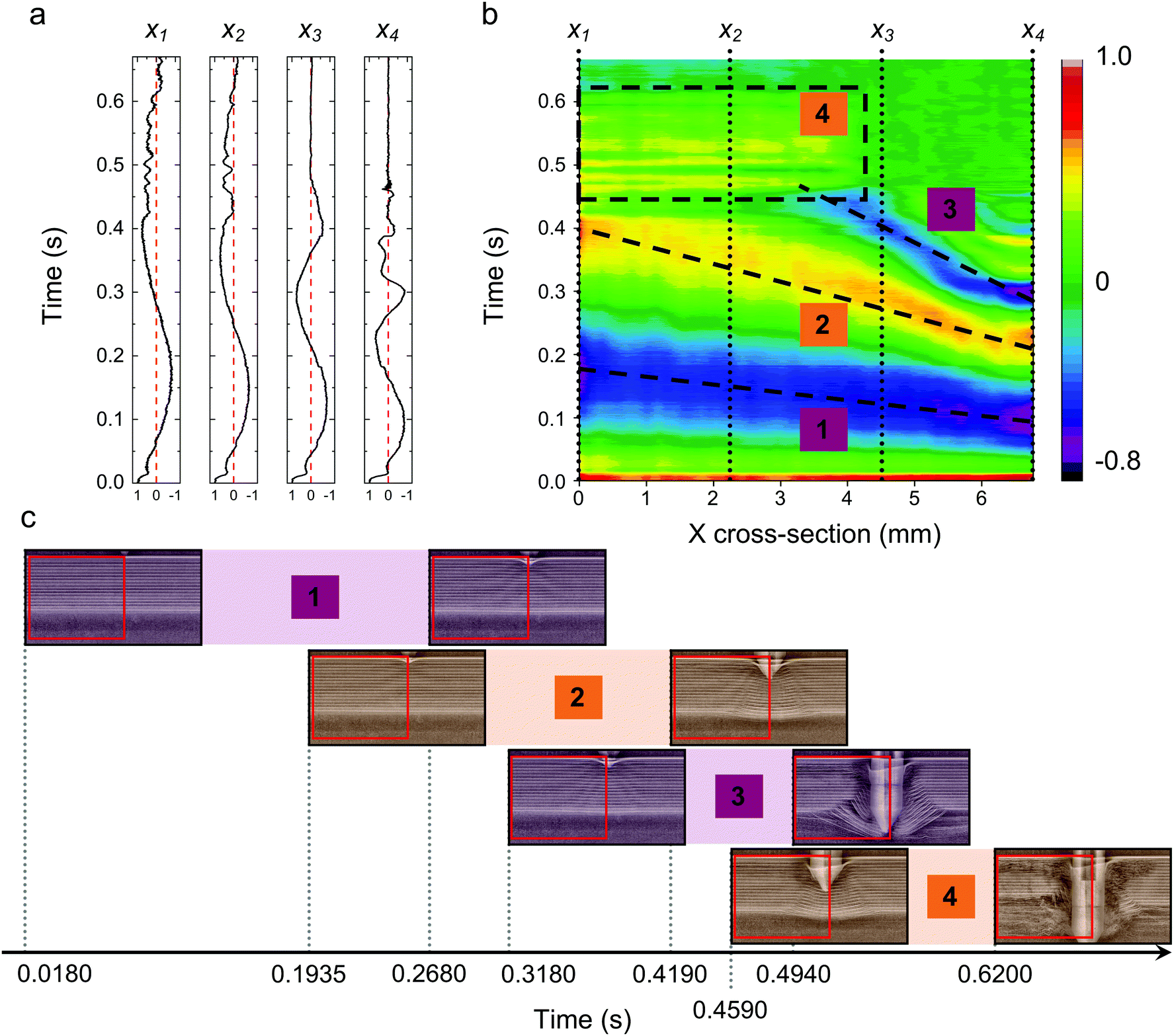

Fig. 6 Various events captured by the spatiotemporal cross-correlation map in the dataset ‘SI_Video_1’ (ESI†). (a) Normalised cross-correlation plots at four X cross-sections, x_1–4 (vertical dotted lines in (b) showing varying effects experienced by the electrodes due to the nail. (b) The 2D spatiotemporal map plotted by calculating the normalised cross-correlation values at every X position (shown in Fig. 7a). (c) Timeline of frames capturing various events picked out from the spatiotemporal map, namely: (1) nail pierces cell casing and starts pushing the electrodes; (2) the top 3–4 electrode layers are mechanically sheared with the onset of failure propagation, while the rest of the electrode structure continue to be displaced. The apparent non-linearity is potentially due to the combination of the mechanical force from the nail and the failure propagation of the top 3–4 electrode layers from the nail (right edge) towards the left edge of the frames; (3) nail fully pierces the electrode layers, which completely fracture, leading to the localised delamination (4) of the bottom 4–5 electrode layers, captured between x = 0 and 4 mm, and t = 0.45 and 0.62 s.

(i) Inspect the map for distinct features, such as continuous regions of a consistent colour (e.g., Event (1) in Fig. 6b), or abrupt axial discontinuities (e.g., Event (4) in Fig. 6b).

(ii) Continuous regions of colour characterise the behaviour of the electrodes across the length of the cell. Linear or non-linear changes to such regions of a colour indicate changes to the electrode structure propagating across the X cross-section over time. For example, the dark blue region near the bottom of Fig. 6b suggests that the electrodes are becoming misaligned with their initial structure, and that it propagates in the negative X direction, where the origin is the top left of the frames (x = 0, y = 0) and the nail enters at the right-edge of the ROI. On the other hand, areas of a constant colour indicate that the electrode structure is not changing. For example, the green region at the top right of Fig. 6b suggests the electrode structure has disappeared and no further change takes place (this corresponds to the presence of the nail in the cell once it has stopped moving).

(iii) Axial discontinuities characterise events that take place simultaneously across the distance corresponding to the width of the feature in X; at a single point in time, the colour changes homogeneously. For example, if the electrodes in a region delaminate altogether, the map would show an abrupt transition to green, as we observe at around 0.42 s in Fig. 6b.

Using the map in Fig. 6b, we have identified four different events occurring in the electrode structure. These events overlap one another in time; a timeline of raw frames is shown in Fig. 6c. Firstly, the map highlights the point of entry of the nail (right edge of the cropped ROI, x ≈ 6.7 mm) at t ≈ 0.04 s, where the electrodes shift from the right edge to the left edge. Event (1), a region of inverted electrode alignment, represents the rate at which the nail pierces the cell casing and displaces the electrodes, although they have not failed structurally at this point. Event (2) highlights the onset of failure, where the top 3–4 electrode layers are sheared by the nail, with the rest of the electrodes continuing to be displaced. This combination of failure-onset and electrode-displacement propagates non-linearly between t = 0.19 s and t = 0.42 s. This also indicates the onset of Joule heating originating from the sheared top 3–4 electrode layers, marking the increase in the internal cell temperature as reported by Finegan et al. (2017).⁶ The region of inverted cross-correlation marked as Event (3) represents the point at which the electrodes fail structurally by fracturing, leading to localised delamination, shown as Event (4). This occurs very rapidly; the colour transition in the mapping appears horizontal, indicating that the delamination occurred almost homogeneously over 4 mm along the X cross-section. This indicates the need to analyse the Gabor signals in the radial direction (as discussed in the sections below).

Fig. 6 demonstrates the strength of spatiotemporal mapping of X-ray radiography data. We can now assess an entire dataset of thousands of video frames, and thus an entire failure experiment with multiple sub-events, in a single picture. From this, we can observe, directly, how each process propagates along the cell, without needing to scroll through the video manually, further validating our analytical technique. The mapping also reveals and resolves processes that may be missed by manual interrogation, such as the distinction between the electrodes shifting, as in Event (1), and the onset of failure, as in Event (2) in Fig. 6b.

We produced spatiotemporal maps using multiple datasets of nail penetration, as well as the ball compression test, to unravel the events occurring in each experiment (Fig. 7). The maps are interpreted as follows:

Fig. 7 2D spatiotemporal cross-correlation mapping as a quantitative technique to track failure propagation. (a) Spatiotemporal map for the same dataset as in Fig. 6b, that of ‘SI_Video_1’ (ESI†). The map shows the nail entering at the right edge (x = 6.7 mm), causing a more pronounced displacement of the electrodes (Fig. 5d). The map also shows multiple events that are distinct from the electrode displacement, such as failure propagation and localised delamination. (b) Spatiotemporal map of dataset ‘SI_Video_2’ (ESI†), where the nail enters the left edge of the analysed X-ray frames (x = 0 mm) at t ≈ 0.1 s. (c) Spatiotemporal map of dataset ‘SI_Video_3’ (ESI†), where the nail traverses in the axial direction, piercing the bottom of the cell. The electrode structure is located between x = 0 and ≈2 mm. At t = 0.34 s, the core (mandrel) detaches from the bottom of the cell as the nail pierces through the cell, displacing the electrodes. (d) Spatiotemporal map of the dataset ‘SI_Video_4’ (ESI†), where a ball compresses the electrode structure. The map indicates that the centre of the ball, x ≈ 3.45 mm, starts displacing the electrodes from t ≈ 0.04 s, where the extent of displacement reduces radially due to the circular profile of the ball.

(a) Radial nail penetration. Fig. 7a and b show the spatiotemporal map of the datasets ‘SI_Video_1’ (ESI†) (also shown in Fig. 6b) and ‘SI_Video_2’ (ESI†), respectively, where the nail enters the cell in the radial direction. It has been previously reported that the tip of the nail can reach 820 °C under these conditions,⁶ with such tests expected to result in hard-shorting that gradually relaxes due to the large surface area of the nail. Here, we chose the ROI such that the nail centre was at the right edge in Fig. 7a (‘SI_Video_1’, ESI†) and at the left edge in Fig. 7b (‘SI_Video_2’, ESI†). The spatiotemporal maps illustrate similar electrode displacements processes. In Fig. 7b the nail enters the ROI at t ≈ 0.1 s. The gradual shift in the electrodes, similar to Event (1) in Fig. 6b and c (‘SI_Video_1’, ESI†), is apparent from the regions of transition from yellow to green between 0.1 s and 0.17 s. This has not previously been resolved quantitatively in the literature. After the nail penetrates the cell casing, the top electrode layers are pierced, and the onset of failure is captured between t = 0.17 s and 0.38 s. This non-linear region is similar to Events (2) and (3) in Fig. 6b and c (‘SI_Video_1’, ESI†), potentially due to the combined effect of failure of the top 2–3 electrode layers and the displacement of the rest of the layers. It has been reported that the onset of this hard-shorting effect is marked by the increase in internal temperature due to Joule heating,⁶ which has been captured by our technique as the rapid non-linear trends in Fig. 7a and b – Events (2) and (3). At t = 0.38 s in Fig. 7b, there is a horizontal shift in cross-correlation from x = 1 mm to the right edge of the frame, representing a rapid failure of the electrode structure (fracture of electrode layers). This dataset, however, did not exhibit localised delamination, in contrast to our observation of Event (4) in the dataset Fig. 6b and c.

(b) Axial nail penetration. Fig. 7c shows the spatiotemporal map for the dataset ‘SI_Video_3’ (ESI†) in which the nail enters in the axial direction, piercing the bottom of the cell. In previous work it was shown that this orientation leads to the highest internal cell temperature during testing (>900 °C), and indeed the cell fails similarly to that of a thermal abuse condition.⁶ This dataset demonstrates the functionality of our analytical approach, irrespective of the direction of incidence of mechanical objects with respect to the electrode structure. Here, the red area in the bottom left corresponds to the bottom of the cell (x = 0 mm to 2.3 mm), with high similarity due to the negligible electrode shifting, as the nail pierces only the cell casing until around 0.13 s. The blue area between x = 2.5 mm and 3.2 mm is outside the cell (and the cross-correlation is appropriately close to 0 as the Gabor signals are ≈0). The entry of the nail causes a gradual shift of the electrodes, so the correlation values reduce, shown as a transition from red to green between 0.13 s and 0.34 s. This is in agreement with the observations of Finegan et al. (2017)⁶ that there was no electrode fracturing due to the minimal tensile strain on the electrode with the parallel propagation of the nail.

At around 0.34 s, the decrease in cross-correlation speeds up, with a transition from green to blue as the nail begins pushing the electrodes. A sudden shift (seen from the horizontal dark blue line) indicates the mandrel detaching from the bottom of the cell, though thermal runaway has still not initiated. This is followed by another region of decreasing cross-correlation close to 0.39 s, where the onset of thermal runaway has been captured with the mandrel starting to disintegrate.

It is worth noting that the slope of this region represents the rate of propagation of thermal runaway for this dataset between 0.39 s and 0.8 s. Subsequently, there was a release of gas into the base of the cell, leading to the bulging of the base plate that then escaped through the vent.

(c) Radial ball compression. For the ball compression test in Fig. 7d, we observe a clear symmetrical electrode displacement centred on the incident location of the ball, x = 3.5 mm. There is a widening pattern of alternating positive (green) and negative (blue) correlation with time. This characterises the shifting of the electrodes under the ball, directly proportional to the distance from the centre of the ball, as previously discussed in Fig. 5a–c. It is interesting to note that this testing condition did not result in thermal runaway, probably due to the relatively large surface area of the ball that distributed the tensile strain axially along the cell. The experimental condition may also not have reached the maximum load-bearing capacity of the cell, as discussed by Wierzbicki and Sahraei (2013).⁴³ Comparing the three nail penetration and ball compression datasets, we observed reproducible spatiotemporal cross-correlation patterns (especially in the radial direction), which may be distinguished as electrode shifting, failure propagation, and rapid delamination, among others. This methodology emphasises the distinct effects that mechanical objects, such as a nail, have on each region of a cell, along with the axial intra-cell effects leading to the propagation of failure within the electrodes. This toolbox, therefore, has the potential to extract and elucidate multiple failure mechanisms that may initiate under abuse testing.

Quantifying the kinetics of failure

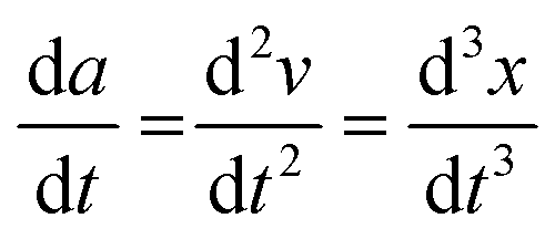
Qualitative assessment of failure has been well-documented in literature and has advised several preventative and mitigative safety considerations for the use of lithium-ion cells. We have demonstrated that, via spatiotemporal mapping of the cross-correlation values, the user obtains a greatly enhanced map of events to produce a more robust understanding of failure. In this section, we realise the true potential of such maps by tracing the trends of multiple events identified in Fig. 6 and 7 for the three nail-penetration test conditions described in Table 1, to advance our mechanistic understanding of the onset of cell failure. From the spatiotemporal maps, we extracted the (x, t) coordinates of each distinctive event described by either a negative cross-correlation region, a positive cross-correlation region, or a sloping region (Fig. 8). We performed third order polynomial regression, equivalent to the Newtonian equations of motion, on these coordinates, to extract the initial jerk (3rd order coefficient), initial acceleration (2nd order coefficient), initial velocity (1st order coefficient) and origin of each event (x intercept). Since the propagation of failure occurs due to the combination of the force imparted by the nail and the initiation of exothermic thermal runaway,^1,44–48 to capture the changing forces/stresses we assume that the rate of propagation of failure can be characterised under a time-dependent acceleration condition, such that:where, a is the acceleration with time, t, and the rate of change of acceleration is jerk, j, assumed to be constant. Further, this can be extended to a well-known form:where v is the velocity and x is the position. In polynomial terms, we can therefore express the change in position over time as:change in velocity over time as:and change in acceleration over time as:

a(t) = a₀ + j₀t (5)

We used three methods to determine the coordinates of each trend, depending on whether we were tracing peaks or valleys. The 2D maps in Fig. 8a–c are the spatiotemporal maps that have been transposed to display time in the horizontal axis and X position on the vertical axis. Our primary approach was to find the peaks (or troughs) of the cross-correlations along x for each point in time. Alternatively, we found the peaks (or troughs) of the correlations along time for each X position. This resulted in multiple X positions for a given time, where multiple x values at each t were averaged and the standard deviation, σ_exp, in x was applied as experimental uncertainty of the data. Our final method, in the case that we needed to trace a gradual shift in the correlation values as opposed to a sudden shift (used for trend (iv) in Fig. 8), was to threshold the colour scale to the correlation values associated with the trend. This isolated a 2D shape containing the trend data, from which we could find the mid-point at each X position. Multiple x values at each t were also averaged and the experimental uncertainty, σ_exp, in x estimated, as in the case above. The bottom row of Fig. 8 shows the resulting data points with the 3rd order polynomial fits. The coefficients of the fits are shown in Table 2.

Fig. 8 Quantification of the kinetics of events in three nail penetration datasets. The 2D spatiotemporal maps have been transposed such that time is on the horizontal axis and X cross-section is on the vertical axis. (a) The regions of low and high cross-correlation values of three events (described in Fig. 6) in the dataset ‘SI_Video_1’ (ESI†), traced using a simple yet robust maxima/minima finding algorithm and their corresponding 3rd order polynomial fits shown in the bottom panel (trends i–iii). (b) Two events relating to electrode shifting and propagation of failure in the dataset ‘SI_Video_2’ (ESI†), identified and traced. The bottom panel shows the 3rd order polynomial fits of these traces (trends iv and v). (c) The rates of electrode shifting in the dataset ‘SI_Video_3’ (ESI†), where the nail traverses along the axial direction of the electrodes, have been quantified as shown in the bottom panel (trends vi and vii). The results of the 3rd order polynomial fitting, corresponding to Newton's equations of motion, are shown in Table 2. Note that (vi) is composed of two smaller sections, due to difficulty in reliable peak-tracing.

Table 2 Results from the 3rd order polynomial fits of the seven trends shown in Fig. 8 from three different nail penetration datasets. The 3rd order polynomial was of the form , where v₀ is the initial velocity term, a₀ is the initial acceleration, j₀ is the jerk and x₀ is the x-intercept representing the origin of the event

Dataset	SI_Video_1 (ESI)			SI_Video_2 (ESI)		SI_Video_3 (ESI)
Trends	i	ii	iii	iv	v	vi	vii
Type of event^a	(1)	(2–3)	(2–3)	(1)	(2–3)	(1)	(1)
a The type of the event refers to the ones described in Fig. 6. Event (1) denotes electrode displacement before onset of failure, Events (2–3) denote the onset of failure propagation and further electrode displacement leading to fracture or delamination
Jerk [mm s^−3]	0.0	0.0	3209.2 ± 102.8	2572.43 ± 23.25	0.0	0.0	871.69 ± 4.74
Acceleration [mm s^−2]	−578.0 ± 29.3	108.43 ± 10.01	−281.48 ± 8.31	514.46 ± 1.41	−34.51 ± 0.71	4.91 ± 0.17	−92.39 ± 0.45
Initial velocity [mm s^−1]	91.66 ± 0.53	22.72 ± 0.38	24.58 ± 0.28	0.0 ± 0.04	9.46 ± 0.03	2.49 ± 0.01	7.49 ± 0.02
Origin of event along x [mm]	0.13 ± 0.01	0.64 ± 0.01	0.64 ± 0.01	0.61 ± 0.01	0.07 ± 0.01	1.75 ± 0.01	1.28 ± 0.01
R ^2	0.82	0.98	0.93	0.98	0.94	0.99	0.99

---

A non-linear least-squares fitting method was used to fit eqn (3) to the averaged x data (regression performed using Python 3, with a convergence tolerance = 1 × 10⁻⁸). The fitting coefficients were constrained such that v₀ is positive, i.e., we define that the events progress in the positive x direction due to the expected unidirectional movement from the nail surface propagating away from the nail. x₀ was constrained 0 ± 2 mm, i.e., events begin within the region defined by the diameter of the nail. For each fit, the model uncertainty (±1 standard deviation) was calculated from the square root of the diagonal of the covariance matrix. The corresponding R² of the fits was also estimated.

Trends (i) and (iv) represent the shifting of the electrodes prior to structural failure for nail penetration in the radial direction. Trend (i) has j₀ = 0, i.e., there is no jerk present and the acceleration is constant, whereas trend (iv) has an initial jerk of 2570 mm s⁻³. Trend (i) has an initial velocity of 91.7 mm s⁻¹ but decelerates at 578 mm s⁻². We note that this deceleration term has quite a large error of ±29 mm s⁻², which might result from the noise in the data. Conversely, trend (iv) has an initial velocity of zero, but accelerates rapidly at 515 mm s⁻² resulting in v(t_0.31) ≈ 250 mm s⁻¹ at t = 0.31 s. This highlights the intrinsic variation between the mechanical processes occurring during nail penetration tests carried under the same conditions.

Trends (ii), (iii) and (v) correspond to the combined effects of failure propagation and electrode shifting. There are also distinct differences in the acceleration and initial velocity of these processes. Trends (ii) and (iii) have accelerations of 108 mm s⁻² and −282 mm s⁻², and initial velocities of 22.7 mm s⁻¹ and 24.6 mm s⁻¹, respectively. They accelerate to a velocity of v(t_0.42) ≈ 62 mm s⁻¹ and v(t_0.45) ≈ 135 mm s⁻¹. Trend (v) appears to be much slower, with an initial velocity of 9.5 mm s⁻¹ decelerating at −34.5 mm s⁻². This again emphasises the broad range of cell failure kinetics that result from nail penetration tests, although inspection of the videos might lead one to conclude that the processes leading up to full electrode destruction are quite similar.

Trend (iii) has a large initial jerk of 3210 mm s⁻³, although (ii) and (v) have j₀ = 0. Trend (iii) has a high jerk potentially due to the rapid delamination of the bottom 3–4 electrode layers captured in the video, leading to a sudden inflexion in the x data. We note that fitting higher order polynomials is sensitive to input data, which in our case are peak traces from spatiotemporal maps extracted from legacy data. This may be overcome with acquisition of higher resolution images at higher frame rates, improving the quality of the peak traces.

We also observe abrupt transitions at 0.42 s in Fig. 8a and 0.37 s in Fig. 8b as the cells fail across their length, which effectively ends trends (iii) and (v). From the spatiotemporal maps the shape of the trends appears to diverge at these points. This end point corresponds to the nail reaching the middle of the cell as the electrodes fracture, so the spreading in the colour map likely indicates a rapid final shift of the electrodes away from the nail before they are destroyed.

Trends (vi) and (vii) characterise the electrode response for the case in which the nail entered the cell in the axial direction, causing reduced tensile strain on the electrodes in comparison to entering in the radial direction. a₀ and j₀ are relatively low in comparison to those for the nail entering in the radial direction. Trend (vi) has j₀ = 0 mm s⁻³, while trend (vii) has j₀ = 872 mm s⁻³. They have accelerations of 4.9 mm s⁻² and −92.4 mm s⁻², and initial velocities of 2.5 mm s⁻¹ and 7.5 mm s⁻¹, respectively. We also do not observe a near-homogeneous electrode shift across the cell. We suspect that this contrast in behaviours is due to the difference in mechanical resistance of the electrode layers in each case. It is interesting to compare this behaviour to the ball compression in ‘SI_Video_4’ (ESI†), wherein the electrodes do not fracture and there is no thermal runaway. Likewise, axial penetration of the nail does not stress the electrodes into fracturing, thus it is likely that when thermal runaway occurs it results from internal shorting caused by the nail.

From our quantification of the failure kinetics, we note that the propagation of structural damage (i.e., at the onset of catastrophic failure or uncontrolled thermal runaway) is slower than previously believed. Ignoring the abrupt and total cell failure, and if a certain specific trend propagation were to travel the entire length of a cell (in our case 65 mm), we may extrapolate the model to estimate the velocities to which the failures would accelerate. In the case of trend (iv), the electrodes would be displaced at a maximum velocity of 396 mm s⁻¹ (v₀ = 0 mm s⁻¹) by t = 0.578 s, traversing the entire length of an 18 650 cell, whereas, a failure trend involving a delamination event, e.g., trend (iii), would traverse the entire length of an 18 650 cell by t = 0.7 s, reaching a maximum velocity of 163 mm s⁻¹ (v₀ = 24.6 mm s⁻¹). This reinforces the view previously put forward by the authors that, counter-intuitively, failure due to nail penetration may not be as severe a mode of failure/abuse as has been reported in the literature.

Tracking the radial propagation of failure processes

So far, we have quantified the propagation of failure and the intra-cell effects in the axial direction. However, it is clear from the spatiotemporal maps that some events happen abruptly, homogeneously across the X cross-section. In these cases, we cannot track the shape of a cross-correlation trend because it describes a process occurring in the radial direction; the transformation from Gabor signals to cross-correlation collapses the information in the y direction into single values at each x position. Thus, events that appear instantaneous on the (x, t) cross-correlation maps can only be quantified by accessing the y coordinate system.

Fig. 9a shows the temporal Gabor signal from the ‘SI_Video_1’ (ESI†) dataset (nail travelling in the radial direction), 3.7 mm from the nail surface (x ≈ 1 mm); similar to that of Fig. 4a which represents the temporal map at the nail surface (x ≈ 4.7 mm). Until around 0.5 s, the electrode structure remains intact with just a gradual shift due to the nail. However, there is then a sudden shift and loss in magnitude in the lower electrode layers, from y = 2.75 mm to 6 mm, which indicates the localised delamination captured in this dataset (Fig. 6b, Event (4)). In order to extract the kinetics of this event, which was very abrupt on the (x, t) spatiotemporal maps, we tracked the net shift of each Gabor peak in the temporal Gabor map (along the y axis).

Fig. 9 Estimation of rate of failure/delamination in the radial direction from the dataset ‘SI_Video_1’ (ESI†). (a) 2D temporal Gabor map showing the evolution of the electrode structure over time (normalised) ≈3.7 mm away from the nail surface (x ≈ 1 mm), similar to that of Fig. 4a (at the nail surface). The point of delamination has been shown in the inset box, which was cropped to extract radial propagation velocities, as shown in (b). (b) The radial shift in electrodes over time was extracted by tracing the Gabor signals over a range of Gabor angles 100°–165° (see ‘SI_Video_7.avi’, ESI†). The most prominent Gabor traces were skeletonised to single-pixel wide lines that denote the rate of delamination. (c) The delamination velocity of each electrode layer was calculated by performing linear regression on the skeletonised lines at every Gabor angle and the distribution plotted.

Fig. 9b shows data manually cropped from Fig. 9a, corresponding to the delamination. This region appears disordered, with electrodes shifting in the positive y direction at different rates. In order to characterise how this failure propagates, we studied the distribution of electrode-shift velocities by capitalising on the power of Gabor filter banks again. We applied a further Gabor filter bank (θ = 100° to 160°) on the temporal Gabor signal data, with a fixed frequency equivalent to the electrode width. For each orientation we obtained an output image highlighting the most prominent trajectory taken by each electrode over time (see ‘SI_Video_7.avi’, ESI†). Fig. 9b shows the segments picked out at three angles, where we can observe a range of trajectories taken by each electrode layer. However, the filter produced some signal even for features that are slightly misaligned with the orientation. The output signals were therefore binarized in order to convert the trajectories into single-pixel-wide skeletal lines, on which a linear regression was performed to extract the velocities. By summing all the pixels of the Gabor-filtered trajectory images for every angle, we also obtain a signal intensity (Fig. 9c, top panel), wherein a higher signal indicates a greater presence of structure aligned with the filter. For a range of velocities of the electrodes per orientation, as shown in Fig. 9c bottom panel, we may use the signal intensity to guide the user to obtain the velocity distribution for angles that produce high signal intensities. Fig. 9c shows the signal intensity plot and associated velocity distribution.

Interestingly, there were two distinct peaks in the intensity, at θ = 110° and 155°. At θ = 100° we captured the top electrode layers at the onset of delamination with a velocity of around 4 mm s⁻¹, while at θ = 162.5° we captured the bottom-most electrodes that delaminated the fastest, at a velocity of 140 mm s⁻¹ leading on to delamination. Above θ = 162.5°, the extracted Gabor lines were that of the noise from the filter and not representative of the temporal electrode shifts. The orientation at θ = 130° was representative of the delamination velocities of most of the electrodes in the cropped ROI, with an average velocity of 13 mm s⁻¹. We suggest that this delamination velocity acts as a point of transition between the electrode shifting due to the force from the nail, and a fully uncontrolled thermal runaway process.

Conclusions

We have demonstrated for the first time that the texture-sensitivity of Gabor filtering is very well-suited to quantifying X-ray radiography data of lithium-ion cell failure tests. We have built an assistive toolbox for the rapid and reproducible analysis of both legacy X-ray synchrotron radiography data and future data, where the user is guided to the exact location and time-point at which interesting events occur. Using the directional sensitivity of the Gabor filter, we were able to not only selectively filter the electrodes, but also select and study other objects, such as estimating the penetration velocity of a nail. Further, upon estimating the displacement profiles of electrodes before failure, we have established a platform that extensively analyses and resolves multiple failure events occurring concurrently. These events have been spatiotemporally mapped on a quantitative scale, where an entire failure testing dataset has been condensed and projected onto a single 2D map with distinguishable events.

The true novelty of this analytical technique is the amount of kinetic information that may now be extracted, relating to the events propagating axially and radially in these datasets. Through proof-of-concept validation of our method via the analysis of distinct battery failure datasets, we observed that the nail penetration event occurs more slowly than previously supposed, indicating that the slower onset of electrode failure might render them less dangerous than instantaneous short-circuiting events or thermally induced degradation events.

With an automated, user-friendly toolbox that helps to reduce human-induced error, several X-ray radiography datasets are currently being processed to elucidate the mechanisms and rates of failure induced by a range of thermal, electrical and mechanical sources. It is worth noting that unique events such as mechanical delamination, gas generation and gas-induced electrode shifting can now be robustly identified and their propagation rates quantified. The toolbox can be applied to existing data available from databanks, such as the one hosted by the National Renewable Energy Laboratory, which can help standardise abuse testing procedures. As a first step, the toolbox directly outputs empirical data describing the mechanics of failure, presenting an opportunity for these data to be applied to mechanical as well as thermal runaway multi-physics models of Li-ion batteries. Our toolbox also has the potential to analyse high-resolution, low frame rate images captured using X-ray CT instruments, highlighting that our technique may not be limited to synchrotron radiography data.

Furthermore, this toolbox will be powerful in helping to couple mechanical models with electrochemical thermal runaway models, when used in conjunction with other electrochemical techniques, such as fractional thermal runaway calorimetry (FTRC).⁴⁹ Despite the lower sampling resolution of FTRC compared to high-speed imaging, with advances in calorimetry measurements, it may be possible for high-resolution FTRC data to be used in conjunction with our toolbox to advance understanding of battery degradation.

In the future, the many advantages of this technique can be further exploited by incorporating the ability to analyse data presented radially, i.e., investigating the failure mechanisms across the ‘jelly-roll’. One possible feature addition to our toolbox would be to apply ‘virtual unrolling’ of the jelly-roll before performing Gabor filtering,⁵⁰ thereby facilitating the analysis of batteries with any form-factor, interrogated in any direction, to truly capture the complex nature of thermal runaway.

Conflicts of interest

There are no conflicts to declare.

Acknowledgements

This work was supported by the Engineering and Physical Sciences Research Council (EP/R020973/1); and the Faraday Institution (Faraday.ac.uk; EP/S003053/1, grant numbers FIRG024 and FIRG028). P. R. S. acknowledges funding from the Royal Academy of Engineering (CiET1718\59). This work was also supported by the National Measurement System of the UK Department for Business, Energy & Industrial Strategy; and was authored in part by the National Renewable Energy Laboratory, operated by Alliance for Sustainable Energy, LLC, for the U.S. Department of Energy (DOE) under Contract No. DE-AC36-08GO28308. The views expressed in the article do not necessarily represent the views of the DOE or the U.S. Government. The failure testing experiments were performed in a controlled environment at ID19 at the ESRF (Grenoble, France).

References

1. D. Doughty and E. P. Roth, Electrochem. Soc. Interface, 2012, 21, 37–44.
2. S. R. Golroudbary, D. Calisaya-Azpilcueta and A. Kraslawski, Procedia CIRP, 2019, 80, 316–321.
3. A. R. Baird, E. J. Archibald, K. C. Marr and O. A. Ezekoye, J. Power Sources, 2020, 446, 227257.
4. D. P. Finegan, E. Darcy, M. Keyser, B. Tjaden, T. M. M. Heenan, R. Jervis, J. J. Bailey, R. Malik, N. T. Vo, O. V. Magdysyuk, R. Atwood, M. Drakopoulos, M. DiMichiel, A. Rack, G. Hinds, D. J. L. Brett and P. R. Shearing, Energy Environ. Sci., 2017, 10, 1377–1388.
5. D. P. Finegan, M. Scheel, J. B. Robinson, B. Tjaden, I. Hunt, T. J. Mason, J. Millichamp, M. Di Michiel, G. J. Offer, G. Hinds, D. J. L. Brett and P. R. Shearing, Nat. Commun., 2015, 6, 6924.
6. D. P. Finegan, B. Tjaden, T. M. M. Heenan, R. Jervis, M. Di Michiel, A. Rack, G. Hinds, D. J. L. Brett and P. R. Shearing, J. Electrochem. Soc., 2017, 164, A3285–A3291.
7. M. Onuki, S. Kinoshita, Y. Sakata, M. Yanagidate, Y. Otake, M. Ue and M. Deguchi, J. Electrochem. Soc., 2008, 155, A794.
8. J. Xu, H. R. Thomas, R. W. Francis, K. R. Lum, J. Wang and B. Liang, J. Power Sources, 2008, 177, 512–527.
9. T. Kawamura, A. Kimura, M. Egashira, S. Okada and J. I. Yamaki, J. Power Sources, 2002, 104, 260–264.
10. D. P. Finegan, E. Darcy, M. Keyser, B. Tjaden, T. M. M. Heenan, R. Jervis, J. J. Bailey, N. T. Vo, O. V. Magdysyuk, M. Drakopoulos, M. Di Michiel, A. Rack, G. Hinds, D. J. L. Brett and P. R. Shearing, Adv. Sci., 2018, 5, 1700369.
11. S. M. Bak, Z. Shadike, R. Lin, X. Yu and X. Q. Yang, NPG Asia Mater., 2018, 10, 563–580.
12. D. P. Finegan, J. Darst, W. Walker, Q. Li, C. Yang, R. Jervis, T. M. M. Heenan, J. Hack, J. C. Thomas, A. Rack, D. J. L. Brett, P. R. Shearing, M. Keyser and E. Darcy, J. Power Sources, 2019, 417, 29–41.
13. J. Lamb and C. J. Orendorff, J. Power Sources, 2014, 247, 189–196.
14. Battery Failure Databank, https://www.nrel.gov/transportation/battery-failure.html.
15. E. Cao, A. N. P. Radhakrishnan, R. bin Hasanudin and A. Gavriilidis, Ind. Eng. Chem. Res., 2021, 60, 10489–10501.
16. R. Mehrotra, K. R. Namuduri and N. Ranganathan, Pattern Recognit., 1992, 25, 1479–1494.
17. H. Kaur and L. Kaur, Int. J. Sci. Res., 2014, 3, 1879–1886.
18. A. Kumar and G. K. H. Pang, IEEE Trans. Ind. Appl., 2002, 38, 425–440.
19. A. C. Bovik, M. Clark and W. S. Geisler, IEEE Trans. Pattern Anal. Mach. Intell., 1990, 12, 55–73.
20. P. Toth, A. B. Palotas, E. G. Eddings, R. T. Whitaker and J. A. S. Lighty, Combust. Flame, 2013, 160, 909–919.
21. M. J. Hÿtch, E. Snoeck and R. Kilaas, Ultramicroscopy, 1998, 74, 131–146.
22. M. Pourfard, K. Faez and S. H. Tabaian, J. Nano Res., 2015, 31, 40–61.
23. A. Talukder and D. P. Casasent, Wavelet Appl. V, 1998, 3391, 336–347.
24. M. Freyer, A. Ale, R. B. Schulz, M. Zientkowska, V. Ntziachristos and K.-H. Englmeier, J. Biomed. Opt., 2010, 15, 036006.
25. N. Homma, K. Takei and T. Ishibashi, WSEAS Trans. Inf. Sci. Appl., 2008, 5, 1227–1236.
26. L. Wiskott, J. M. Fellous, N. Krüger and C. Von der Malsburg, Lect. Notes Comput. Sci., 1997, 1296, 456–463.
27. J. Yang, L. Liu, T. Jiang and Y. Fan, Pattern Recognit. Lett., 2003, 24, 1805–1817.
28. J. Zhu, W. Li, T. Wierzbicki, Y. Xia and J. Harding, Int. J. Plast., 2019, 121, 293–311.
29. J. Zhu, M. M. Koch, J. Lian, W. Li and T. Wierzbicki, J. Electrochem. Soc., 2020, 167, 090533.
30. C. Zhang, S. Santhanagopalan, M. A. Sprague and A. A. Pesaran, J. Power Sources, 2015, 298, 309–321.
31. X. Feng, X. He, M. Ouyang, L. Wang, L. Lu, D. Ren and S. Santhanagopalan, J. Electrochem. Soc., 2018, 165, A3748–A3765.
32. T. D. Hatchard, S. Trussler and J. R. Dahn, J. Power Sources, 2014, 247, 821–823.
33. G. van Rossum, Python tutorial, Technical Report CS-R9526, Amsterdam, 1995.
34. S. Silvester, A. Tanbakuchi, P. Müller, J. Nunez-Iglesias, M. Harfouche, A. Klein, M. McCormick, OrganicIrradiation, A. Rai, A. Ladegaard, A. Lee, T. D. Smith, G. A. Vaillant, jackwalker64, J. Nises, rreilink, H. van Kemenade, C. Dusold, F. Kohlgrüber, G. Yang, G. Inggs, J. Singleton, M. Schambach, M. Hirsch, M. Komarčević, N. Rosenstein, P.-C. Hsieh, Zulko, C. Barnes and A. Elliott, imageio DOI:10.5281/zenodo.4972048.
35. S. van Der Walt, S. C. Colbert and G. Varoquaux, Comput. Sci. Eng., 2011, 13, 22–30.
36. T. E. Oliphant, Comput. Sci. Eng., 2007, 9, 10–20.
37. S. van der Walt, J. L. Schönberger, J. Nunez-Iglesias, F. Boulogne, J. D. Warner, N. Yager, E. Gouillart and T. Yu, PeerJ, 2014, 2, e453.
38. J. D. Hunter, Comput. Sci. Eng., 2007, 9, 90–95.
39. F. Lundh, http://www.pythonware.com/library/tkinter/introduction/index.htm.
40. Google, Tesseract, https://tesseract-ocr.github.io/.
41. Pytesseract, https://pypi.org/project/pytesseract/.
42. A. N. P. Radhakrishnan, M. Pradas, E. Sorensen, S. Kalliadasis and A. Gavriilidis, Langmuir, 2019, 35, 8199–8209.
43. T. Wierzbicki and E. Sahraei, J. Power Sources, 2013, 241, 467–476.
44. M. Gikas and J. Beilinson, 2017, http://www.consumerreports.org.
45. C. Lin, Y. Piao, Y. Kan, J. Bareño, I. Bloom, Y. Ren, K. Amine and Z. Chen, ACS Appl. Mater. Interfaces, 2014, 6, 12692–12697.
46. P. Röder, N. Baba and H.-D. Wiemhöfer, J. Power Sources, 2014, 248, 978–987.
47. D. P. Abraham, E. P. Roth, R. Kostecki, K. McCarthy, S. MacLaren and D. H. Doughty, J. Power Sources, 2006, 161, 648–657.
48. D. P. Finegan, M. Scheel, J. B. Robinson, B. Tjaden, M. Di Michiel, G. Hinds, D. J. L. Brett and P. R. Shearing, Phys. Chem. Chem. Phys., 2016, 18, 30912–30919.
49. D. Patel, J. B. Robinson, S. Ball, D. J. L. Brett and P. R. Shearing, J. Electrochem. Soc., 2020, 167, 090511.
50. M. D. R. Kok, J. B. Robinson, J. S. Weaving, A. Jnawali, M. Pham, F. Iacoviello, D. J. L. Brett and P. R. Shearing, Sustainable Energy Fuels, 2019, 3, 2972–2976.

---

Footnote

† Electronic supplementary information (ESI) available. See DOI: https://doi.org/10.1039/d1ee03430h

---