
 Open Access Article
 This Open Access Article is licensed under a
 Creative Commons Attribution 3.0 Unported Licence
Towards automation of operando experiments: a case study in contactless conductivity measurements†
Peter
Kraus
 *ab,
Elisabeth H.
Wolf
ad,
Charlotte
Prinz
c,
Giulia
Bellini
a,
Annette
Trunschke
a and
Robert
Schlögl
ad
*ab,
Elisabeth H.
Wolf
ad,
Charlotte
Prinz
c,
Giulia
Bellini
a,
Annette
Trunschke
a and
Robert
Schlögl
ad
aAnorganische Chemie, Fritz-Haber-Institut der Max-Planck-Gesellschaft, Faradayweg 4-6, 14195 Berlin, Germany
bSchool of Molecular and Life Sciences, Curtin University, GPO Box U1987, Perth 6845, WA, Australia. E-mail: peter.kraus@curtin.edu.au
cElektroniklabor, Fritz-Haber-Institut der Max-Planck-Gesellschaft, Faradayweg 4-6, 14195 Berlin, Germany
dHeterogenous Reactions, Max-Planck-Institut für Energiekonversion, Stiftstr. 34-36, 45470 Mülheim an der Ruhr, Germany
First published on 28th February 2022
Abstract
Automation of experiments is a key component on the path of digitalization in catalysis and related sciences. Here we present the lessons learned and caveats avoided during the automation of our contactless conductivity measurement set-up, capable of operando measurement of catalytic samples. We briefly discuss the motivation behind the work, the technical groundwork required, and the philosophy guiding our design. The main body of this work is dedicated to the detailing of the implementation of the automation, data structures, as well as the modular data processing pipeline. The open-source toolset developed as part of this work allows us to carry out unattended and reproducible experiments, as well as post-process data according to current best practice. This process is illustrated by implementing two routine sample protocols, one of which was included in the Handbook of Catalysis, providing several case studies showing the benefits of such automation, including increased throughput and higher data quality. The datasets included as part of this work contain catalytic and operando conductivity data, and are self-consistent, annotated with metadata, and are available on a public repository in a machine-readable form. We hope the datasets as well as the tools and workflows developed as part of this work will be an useful guide on the path towards automation and digital catalysis.
1 Introduction
Heterogeneous catalysis is a complex, multiscale phenomenon. The understanding of catalysis is particularly complicated on metal-oxide materials, where the catalytically active site may appear only under operating conditions, as a component of a dynamically formed, kinetically frustrated phase.1 That is why the importance of operando experiments as investigative probes of the active state of the system cannot be overstated. To ensure interpretability and reproducibility of the obtained experimental results, the instrumentation as well as the collection of data and associated metadata should be automated.2 The use of reproducible protocols and automation during the synthesis, characterisation, and associated benchmarking of catalysts is common in the industry.3 Of course, within the proprietary context, such data is rarely shared.3 From an academic point of view, the German Catalytic Society (GeCatS)4 as well as the Swiss National Centre for Competence in Research in Catalysis (NCCR Catalysis)5 have recently focused on digitalization of catalysis. Within the vision of GeCatS, digitalization is a process that allows to compile and mine data for various catalysts, describe and understand the complexity of catalysis, predict improved catalysts, develop improved reactor designs, and optimize process conditions.4 As part of this process, the importance of operando methods for investigation of catalysts as well as the digitization and standardisation of the resulting data is strongly emphasized. As a result, several consortia (e.g. NFDI4Cat, FAIRmat) and initiatives (e.g. NOMAD, Materials Project) have been proposed and established to tackle these challenges systematically. However, the importance of smaller-scale efforts intended to boost the amount of openly available data in the short term has also been highlighted.2In our previous work, we have proposed a set of best practices in designing catalytic testing protocols, and suggested a minimum characterisation standard of materials, both codified in a Handbook for Catalysis.6 Protocols for catalytic testing in partial oxidation of lower alkanes are defined in this Handbook, including the partial oxidation of propane (C3H8) in the optional presence of steam, yielding value-adding products such as propylene (C3H6) or acrylic acid (C2H3COOH), or unwanted combustion products such as CO, CO2 and H2O:
 | (1) |
In this work we discuss the practicalities of applying the protocols defined in the Handbook to an operando experiment: a contactless operando measurement of electrical conductivity using the microwave cavity perturbation technique (MCPT).7 MCPT allows for the concurrent investigation of the electrical, dielectric, and catalytic properties of a catalytic system. This is achieved by placing the reactor, including the catalyst and reactant gases, into a cylindrical microwave cavity. The dielectric properties of the system can then be deduced from the perturbations of the quality factor of the cavity. The technique is therefore complementary to X-ray photoelectron spectroscopy (XPS), providing information about the changes of conductivity and permittivity of the overall system at ambient pressure as a function of temperature, feed composition, or feed residence time.8 Using MCPT, we can infer information about the nature of the charge carriers and the electronic structure from the direction and magnitude of the MCPT response to the imposed conditions. The importance of electrical conductivity as a potential descriptor of selectivity in vanadium catalysts has been previously discussed elsewhere.9,10
Here, we first discuss the automation of the MCPT instrument, and the improved reliability of the experiments and the uptime of the MCPT instrument by the use of a second cavity mode acting as an internal standard. A discussion of the approaches to automation during the data collection, data processing, and quantification of experimental errors follows. These improvements allow for a routine application of the technique using standardized operando test protocols.6 In the second part of this work, we highlight the quality of data obtained with the improved instrument using several examples and comparisons with previous results, and present two datasets of operando conductivity data in propane oxidation (eqn (1)) over various metal oxides as well as perovskites.
2 Methods
In the following section, we first outline the previous MCPT set-up and discuss the improvements to the hardware that underpin the automation work. Second, we summarize the working principle of MCPT and its use as a method for measuring electrical conductivity, and provide the revised equations necessary to process the raw instrumental data. In the third section, we discuss the motivation and design choices behind the automation of the instrument, focusing on the operator's point of view. Fourth, we present our strategy for automated data and metadata collection, data processing and error estimation, with emphasis on transparency and interoperability. Finally, we discuss the two sample protocols used in this work, and present the characterisation data of the materials investigated using the MCPT set-up.2.1 MCPT set-up
The details of the previous version of the MCPT set-up were first reported by Eichelbaum et al.7 A simplified block diagram of the instrument is shown in Fig. 1; a detailed instrument diagram along with a list of the key equipment for the current, revised arrangement is shown in the ESI.† | ||
| Fig. 1 A simplified block diagram of the gas flows in the MCPT instrument. | ||
Under normal operation, the inlet gases, controlled by a set of mass flow controllers (Bronkhorst), are mixed, pre-heated using a heating tape (Horst, 140 °C setpoint), and enter a cylindrical glass reactor (3 mm internal diameter, Ilmasil PN, Quarzglas Heinrich Aachen) where they pass over the studied sample. The glass reactor is connected to a Swagelok pipe at both ends using Ultratorr fittings. The reactor is horizontally mounted in a glass dewar (HSQ100, Quarzglas Heinrich Aachen), forming three separated layers when assembled: the reactor tube is filled with the flowing reactant gas mixture passing over the sample, the middle layer contains the flowing heating medium (air, 11 l min−1), and the final insulating layer of the dewar is pumped down to vacuum (∼ 10−7 mbar). The dewar/reactor assembly is mounted in the microwave cavity. The piping connecting the rear outlet of the reactor with the gas analyser is heated by a heating tape (Horst, 140 °C setpoint) and the product gases are analysed online by a gas chromatograph (Agilent 7890 GC), equipped with a thermal conductivity detector (TCD) and a polyarc flame ionisation detector (FID).
The dielectric behaviour of the system is measured using a vector network analyser (VNA, Agilent PNA-L N5320C) coupled to the cavity using a coaxial cable connected to the S11 port, i.e. in reflection mode. The cavity used in the current study is made of copper, plated with silver and gold, with a height (hc) of 20 mm and a radius (rc) of 34 mm.11 The dewar/reactor assembly crosses the centre of the cavity in the axial direction, with two more openings in the cavity in the radial direction: one is occupied by the coupling loop, while the other one acts as an inlet for a N2 purge stream (15 ml min−1) which helps to reduce condensation in the cavity. The cavity is cooled to 18 °C by a set of Peltier elements. The coolant for the Peltier elements is kept at 23 °C using a thermostat (Julabo Corio CD-200 F) to reduce measurement errors by maintaining a duty cycle of the Peltier elements above zero at low thermal loads.
To further reduce noise in the measurements, the cavity is mounted on a 5 mm thick piece of rubber to reduce vibrations, and the network analyser is separated from the mains network by an uninterruptible power supply (Eaton 5PX 2200). With the exception of the sample loading process, the operation of the instrument has been completely automated (see Section 2.3). The output of the air heater is regulated by a type K thermocouple inserted into the glass reactor but outside of the cavity, in front of the sample. The metallic thermocouple cannot be inserted into the cavity, as it would interfere with the measurement of conductivity. The temperature shift between this thermocouple and the centre of the catalytic section is calibrated using a separate thermocouple in an empty reactor with a 5 ml min−1 flow of N2. The temperatures at the ends of the catalytic zone can therefore vary by ±5 °C, and any endo- or exothermicity of the catalytic reaction is not taken into account. The Peltier elements used for cooling of the cavity are regulated by a third thermocouple, mounted to the front plate of the cavity. The power to the air heater (Serpentine III F017558) as well as the cooler is provided from a separate circuit, and is regulated by a purpose-built heater controller (based on Eurotherm 3504). The temperatures, along with the flows of individual reaction gases as well as the flow of the gas mixture, can be regulated and pre-programmed using a custom-made Labview interface (see Section 2.3).
A necessary pre-requisite to allow automated operation of the instrument was to ensure a safe unattended operation. In addition to the standard gas safety practices, instrument-specific risk mitigation strategies include the use of an uninterruptible power supply to ensure a safe shut-down of the computer, heater controller, and gas flows. The purpose-built heater controller ensures instrument safety by: (i) monitoring the flow of the heating medium using a separate flow meter (SMC PFM 725); (ii) monitoring any changes in the resistivity of the heater element (Serpentine III F017558), and (iii) monitoring the temperature of the flow against a maximum value hard-coded in the firmware of the heater controller (550 °C). Triggering either of the three thresholds immediately cuts power to the heater and replaces the current gas mixture with an inert purge. Instrument operation can then only be restored using a physical reset button on the heater controller.
2.2 MCPT theory
In previous investigations, the electrical conductivity (σ) was measured using the TM110 mode7,12 and later the TM010 and TM020 modes8,11 of the cavities. For the TM0n0 modes, the electrical field maximum is in the radial centre of the cavity as shown in Fig. 2. The shape of the field does not change axially along the cavity (i.e. along the catalytic bed). This means the interaction of the field with the system is dominated by the interaction of the field with the material at the centre of the cavity (i.e. the dewar/reactor assembly and the catalytic bed). On the contrary, the TM210 mode, also shown in Fig. 2, has a node at the radial centre of the cavity, with four equivalent field maxima located between the centre of the cavity and the cavity walls. This mode is significantly affected by the cavity itself as opposed to the dewar/reactor assembly in the centre. Therefore, it can be used as a proxy measure of the changes in the cavity during the experiment.13 As the frequency of the TM210 mode is always in the vicinity of the TM020 mode (given by the roots of the corresponding Bessel functions, which are ∼5.1356 and ∼5.5201, respectively), the two modes can be measured conveniently in a single frequency sweep of the network analyser. | ||
| Fig. 2 Comparison of the magnitude of the electric fields in the TM020 and TM210 modes. | ||
The properties of the cavity, i.e. the quality factors (Q) and the resonance frequencies (f) of the two modes are obtained by fitting the reflection coefficient, measured as a function of frequency (Γ(f)), using a Python version of Kajfez's program Q0REFL,14 see Section 2.4. In order to use the parameters obtained for the TM210 mode as a reference for the TM020 mode, the observed resonance frequency fTM210 has to be appropriately scaled up to model the reference frequency of the TM020 mode in an equivalent empty cavity (f0). It is possible to use measured data from a cavity without a sample and fit the scaling factor,13 but we prefer to use the ratio of the Bessel function roots (eqn (2)) to reduce the number of empirical parameters.
 | (2) |
Unfortunately, no such scaling is available for the quality factor. The measured quality factor of the cavity, fitted with a dewar and a reactor, heated up to 400 °C and under ∼10−7 mbar pressure is QTM020,r = 3956 ± 10. At the beginning of every measurement, the current quality factor of the TM210 mode with the sample inserted is recorded under inert conditions, or as specified in the applicable protocol (see Section 2.5), and a scaling ratio Qfac is calculated according to eqn (3).
 | (3) |
Then, the scaled quality factor corresponding to an empty cavity (Q0) is calculated using Q0 = QTM210 × Qfac for the remainder of the experiment. The MCPT parameters realated to the sample (fs and Qs) are obtained directly from the fit to the TM020 peak, as in previous work.8
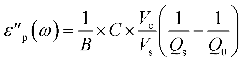
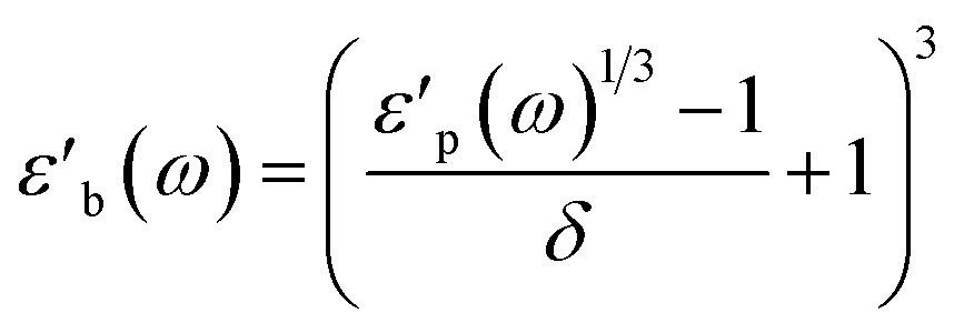
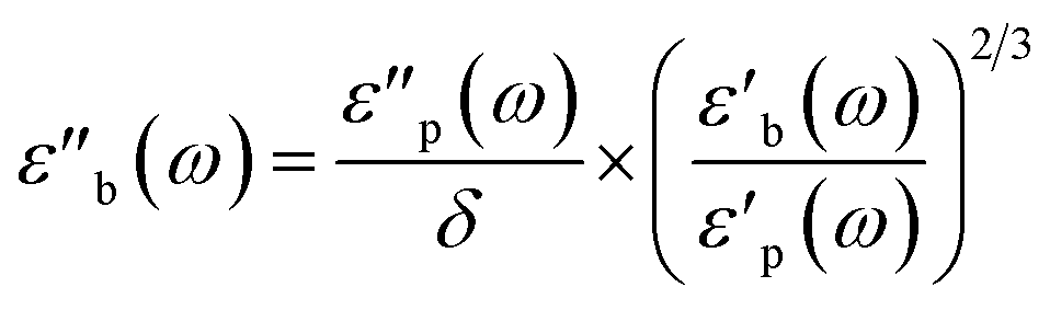
The real and imaginary part of the complex permittivity (ε) of the system are calculated according to eqn (4) and (5). The constants A, B, C were previously empirically fitted to match reference experimental data using single crystals and powders.7 In the current work we reduced the number of fitted parameters by applying A = 1, B = 2, with only C fitted. With C = 0.07 we obtain a good match with the previous experimental data on V2O5.8 The variables Vc = πrc2hc and Vs = πrs2hs are the volumes of the cavity and the sample, respectively.
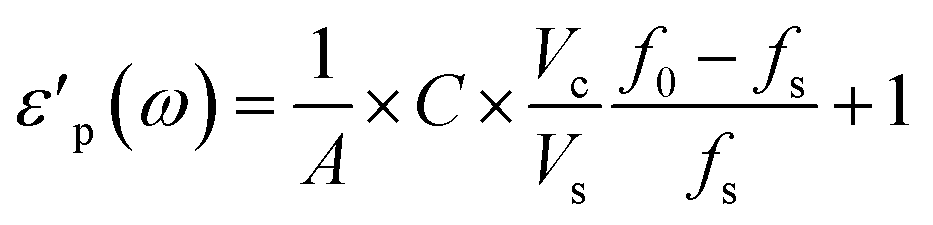 | (4) |
 | (5) |
 | (6) |
 | (7) |
 | (8) |
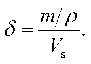 Strictly speaking, δ should be determined using the bulk density of the sample instead of the crystallographic density. However, with limited sample amounts, the determination of bulk densities that would be representative of the packing in the reactor is challenging, and as the crystallographic densities were available for all samples, we have decided to use those instead. The real part of the frequency dependent conductivity
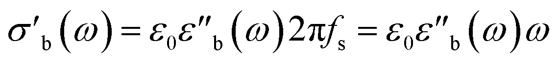
  is then calculated from the imaginary part of the bulk-like permittivity
  the permittivity of vacuum ε0, and the angular frequency ω = 2πfs.
2.3 Instrument automation
The practice of automating laboratory instruments is of course well established. For short reviews on the history of automation in clinical chemistry laboratories and in chemical process development, we refer the reader to ref. 17 and 18, respectively. The field is fast-moving, but with a clear focus on areas of chemistry other than catalysis, mainly in the areas of biochemistry,17,19 high-throughput and parallel experimentation for drug design,18,20 and automated synthesis in flow reactors.21,22Our motivation behind the automation of the instrument was two-fold. The first set of reasons were the intrinsic benefits of automation (see e.g. Ref. 23): an increased reproducibility of experiments by eliminating sample-to-sample variability introduced by human inputs, an increased ease of repeated analysis as complex sample protocols can be reused many times after their definition, and a decrease in the barrier for implementing seamless data collection and logging of metadata. The second set of reasons was much more pragmatic: an automated instrument is able to perform longer and uninterrupted experiments, it can be monitored off-site, and the only manual task in the workflow – the insertion of the sample into the reactor – can be predictably scheduled.
Among the many available platforms for instrument automation, two were considered for implementation in greater detail: Python and LabView. The advantages of a Python implementation are the zero licensing costs for the platform, its widespread use in scientific software, and a comparably easy interface with the data-processing routines, which were also written in Python (see Section 2.4). On the other hand, the key advantages of LabView are the availability of instrument drivers supplied by equipment vendors, the ease by which a graphical control interface can be developed, and the visual programming paradigm of LabView, which is more accessible for non-experts. The development of an accessible, efficient, and dependable user interface is a key factor for the success of any automation project,24 leading us to choose LabView. An additional advantage of the LabView platform in our particular case was its use in other projects in the department, including in the development of the modular iKube reactor (premex reactor GmbH). Of course, by combining a LabView-based automation interface with post-processing tools written in Python, one loses some benefits of each platform: the software stack has a non-zero licensing cost, and modifications of the post-processing software require a different skillset than the modifications of the automation interface. However, the combination of the two platforms allowed us to develop both the automation and the post-processing software rather quickly, independently from each other, with the more appropriate tool for each task.
The current version of the interface is shown in Fig. 3. On the right side, highlighted in green, is the manual control interface, which follows the general design principles outlined in ref. 24. The interface is able to control the heater circuit (A), the cavity cooling using Peltier elements (B), the gas flow settings (C), settings of the vector network analyzer (D), and internal logger settings (E). The heating/cooling panels (A) and (B) are interfacing with the Eurotherm 3504 control unit, and allow for reading and setting the temperature setpoints and a heater ramp. Panel (A) includes a trip alarm light that cannot be overriden using software (discussed in Section 2.1). The gas flow control in panel (C) interacts with a Bronkhorst Flowbus unit, schematically showing the piping arrangement. The readouts as well as the units are obtained automatically by probing the Flowbus. In panel (D), all settings relevant to data collection using the network analyzer can be modified. Finally, panel (E) allows the user to log setpoints and readouts by specifying a path of the instrument log file and the logging frequency. A sample instrument log output is shown in Fig. S1.† This panel also triggers the asynchronous recording of the network analyser signal into a separate VNA log file, applying the settings in panel (D). A sample VNA log is shown in Fig. S2.†
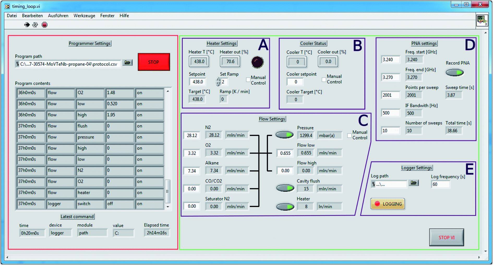 | ||
| Fig. 3 Instrument control interface. Green panel: manual instrument control. Red panel: programmable interface. See text for further details. | ||
All of the above parameters can be programmed using the panel on the left side of Fig. 3 (red highlight). This panel allows the user to load an instrument protocol file (in semicolon-separated-values (SSV) format, see Fig. 4) containing timestamped commands. The interface shows an overview of the loaded commands and also shows the last executed command. The programmer can be stopped, re-started, and overridden using the manual controls in panels (A)–(E), without having to stop the instrument logging. The “manual control” checkboxes in panels (A)–(C) prevent the accidental modification of set-points during an automated run. The LabView virtual instrument (VI) files are available under DOI: http://10.5281/zenodo.5571298.
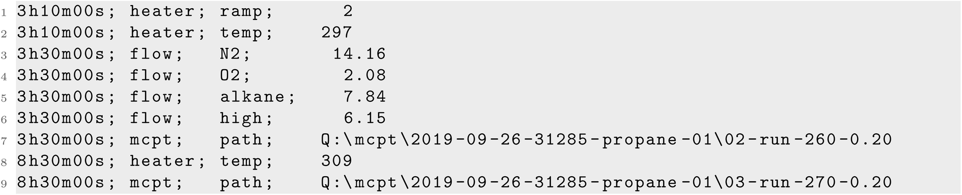 | ||
| Fig. 4 Excerpt from an instrument protocol file, showing an example of setting a ramp reaching 297 °C at 2 °C min−1 (1–2), after 20 minutes adjusting the flow mixture (3–6) and modifying the network analyzer output folder path (7), and finally after 5 hours adjusting the temperature (8) and output folder path (9) again. | ||
The instrument protocol file as well as the instrument log files are complemented by manual entries into the instrument lab book. Ideally, an electronic lab book software would be employed allowing an automated cross-linking between data,20 with the added benefit of enforcing that a run protocol is filled prior to data collection.24 Alternatively, such as in our case, a paper-based run protocol form was developed for each standardized experiment, as shown in Fig. 5. The yellow areas indicate fields that ought to be filled by the operator. Note the entries for calibration files used in the temperature, flow setpoint, MCPT, as well as the GC sections. The run protocol was then digitized and the hard-copy was archived along the instrument lab book. The digitized run protocols are included alongside the processed instrumental data in the ESI.†
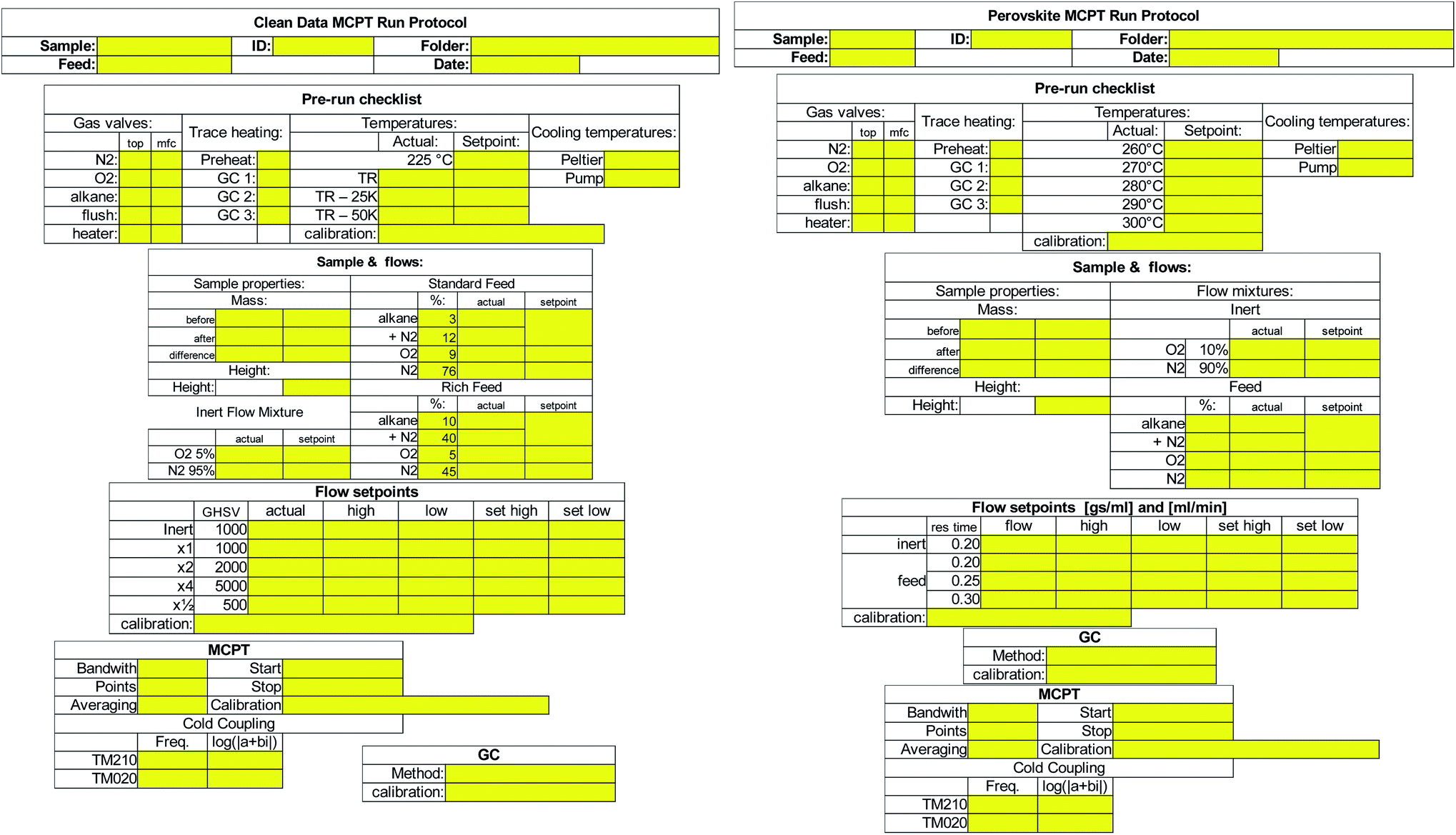 | ||
| Fig. 5 MCPT run protocols for a sample analysis according to the Handbook procedure (left) and procedure used for perovskite samples (right). | ||
2.4 Data collection: from raw data to datagrams
All raw data (VNA logs, instrument protocols and instrument logs, as well as chromatograms automatically exported in ASCII format) are automatically stored on a network-accessible read-only drive, using a timestamped folder structure, with regular backups. The processing of the three data streams (VNA logs, instrument logs, chromatograms) is performed using a set of open-source tools available on Github in two stages. Some of the design principles applied during the development of the tools as well as the nomenclature used in our work are strongly influenced by the QCARCHIVE project, developed by the MOLSSI.25In the first stage, shown in Fig. 6, the yadg tool is used to merge the three data streams into a single datagram file in json format, using the prescription specified in the schema file. The calibration data are specified in the schema, and may be provided in a separate file, which makes them easily exchangeable. The yadg tool allows for the conversion of the setpoints and readouts in instrument logs to time, temperature, pressure, inlet composition, and inlet mass flow rate; the conversion of the frequency dependent reflection coefficient Γ(f) from the VNA logs to quality factors Q and frequencies f used in the MCPT equations; and for the integration and conversion of the peak areas in the chromatograms into the outlet composition. All datapoints within the datagram are timestamped using Unix time format (seconds since the midnight that begins the 1st of Jan. 1970), which allows for a facile calculation of time differences between datapoints, and plotting several datagrams on a single time axis. A Binder-ready Jupyter notebook showing the usage of yadg is included under DOI: http://10.5281/zenodo.5895962. Both the schema and the datagram files are in JSON format, containing an array of dictionaries. The JSON standard is used as it is compact (cf. XML), human-readable (cf. HDF5), flexible (cf. CSV or SSV), and Pythonic. Other formats may be more suitable for different applications, especially if high performance is necessary. The data structure within the schema file is processed separately and sequentially, with a direct 1![[thin space (1/6-em)]](https://www.rsc.org/images/entities/char_2009.gif) :1 map between the schema and the datagram. The elements of the array within the schema describe the nature (instrument log, VNA log, chromatogram) and location (path to file or a folder with files) of the source data, as well as any parameters, calibration data, or calibration files to be applied. The elements of the array within the datagram contain three entries: input, which contains the portion of the schema used to derive the contents; metadata, which contain information about the version of yadg used, path to the schema file, and the date and time of processing; and results, which is an array of timestamped datapoints that were contained within the files/folders specified by the schema. We would like to note that the run protocols, shown in Fig. 5 and discussed in Section 2.3, were tailored to contain all relevant information for specifying the schema.
:1 map between the schema and the datagram. The elements of the array within the schema describe the nature (instrument log, VNA log, chromatogram) and location (path to file or a folder with files) of the source data, as well as any parameters, calibration data, or calibration files to be applied. The elements of the array within the datagram contain three entries: input, which contains the portion of the schema used to derive the contents; metadata, which contain information about the version of yadg used, path to the schema file, and the date and time of processing; and results, which is an array of timestamped datapoints that were contained within the files/folders specified by the schema. We would like to note that the run protocols, shown in Fig. 5 and discussed in Section 2.3, were tailored to contain all relevant information for specifying the schema.
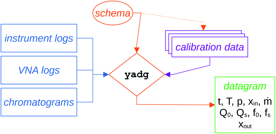 | ||
| Fig. 6 Flowchart of the first stage in the data processing, using yadg. | ||
The obtained datagrams can then be post-processed, based on the required analysis (see Section 2.5) as illustrated in the flowchart shown in Fig. 7. A key item is the parameter file, which contains ESI† about the microwave cavity (cavity radius (rc), cavity height (hc), the reference Q factors (QTM020,r and QTM210,r)), the constants A, B, and C from eqn (4) and (5), the ratio of Bessel function roots jm,n/jμ,η from eqn (2), and the sample parameters (name, sample ID, repetition number, sample radius (rs), sample height (hs), sample mass (m), and the crystallographic density of the material (ρ)). Again, some of the latter parameters are recorded in the corresponding run protocol, see Fig. 5. The entries in this parameter file are formatted to include measurement uncertainties as well as units.
 | ||
| Fig. 7 Flowchart of the second stage in the data processing, transforming the datagram file to processed data. | ||
The main elements of the flowchart in Fig. 7, i.e. the datagram, the parameter file, and the dg2json and dg2png tools, are purposefully kept separate from each other: the datagram contains only data that is recorded by the MCPT instrument, and the parameter file provides data from other measurements that is required to interpret the MCPT results. Notably, neither dg2json nor dg2png contain any data, keeping the data separate from the tools used for analysis (dg2json or dg2png).
As shown in Fig. 7, the dg2json tool is used to post-process the datagrams using supplemental parameters from the parameter file, obtaining a JSON-formatted output file which can be further analysed (directly, using e.g. Jupyter notebooks, or upon conversion to CSV in any spreadsheet software). Indeed, most of the figures in the Results section were prepared this way, see the ESI.† However, sometimes one may wish to have a quick visual overview of the data in one or multiple datagrams, or generate automated reports. For this, the dg2png tool can be used, producing pre-formatted figures which show the operating conditions, catalytic performance, as well as the conductivity of the sample as a function of time. A representative example is shown in Fig. 8, where a normalized conductivity (σ/σr, where σr is determined at 225 °C and 5% O2 in N2 during step 1 of the Handbook protocol, see below) is plotted along propane conversion (Xp(C3H8), subscript “p” denotes a product-based conversion obtained from FID data, as specified by the Handbook).
 | ||
| Fig. 8 A sample PNG file generated using the dg2png tool. Top panel shows the conductivity data (grayscale, left) and propane conversion (blue symbols, right). The bottom panel shows the temperature (black, left), and the gas space velocity (green, right) as well as the inlet mixture (propane in red, oxygen in blue, both right). | ||
2.5 Post-processing: from run protocols and datagrams to results
The final post-processing depends heavily on the type of investigation performed, and different presets for the dg2json tool have been developed for each analysis. As shown in Fig. 5, here we present results based on two types of run protocols: the Handbook procedure, and the perovskite protocol.The Handbook procedure for MCPT investigations is described in the ESI† of ref. 6, with the key reaction shortly summarised in eqn (1). The design of the Handbook MCPT experiment is closely related to the Handbook catalytic testing protocols, as both follow a similar set of conditions, intended to investigate the steady-state behaviour of the catalyst.6 The stages of the experiment are shown in Fig. 9, measuring the catalytic performance as well as the operando conductivity of the catalyst as a function of gas hourly space velocity (GHSV) in steps 2–5, temperature variation in steps 6–8, and feed variation in steps 9–11. Note that steps 2, 6, and 9 correspond to the same conditions, which is important for confirming the reversibility of the observed processes as well as for detecting any drift in the measurement.
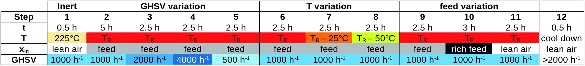 | ||
| Fig. 9 Stages in a Handbook MCPT experiment. TR corresponds to the temperature at which the catalyst shows ∼ 30% conversion, with a maximum of 450 °C. “Lean air” is 5% O2 in N2, “feed” is 3% C3H8 and 9% O2 in N2, and “rich feed” is 10% C3H8 and 5% O2 in N2. | ||
For each step in Fig. 9, the following properties are derived: the inlet mixture composition (xin) and inlet parameters (fuel-to-air equivalence ratio (ϕ), flow rate (![[small nu, Greek, dot above]](https://www.rsc.org/images/entities/i_char_e154.gif) ), residence time (τ), GHSV, temperature (T)), the electrical and dielectric properties
), residence time (τ), GHSV, temperature (T)), the electrical and dielectric properties  as well as the composition of the outlet mixture (xout), and the catalytic properties (reactant and product as well as carbon and oxygen based conversions Xr, Xp, XO,r and XO,p, as well as carbon based selectivities Sp). As the Handbook specifies that steady state properties are to be measured, the post-processing performed when dg2json is used with the Handbook preset reports the means and standard deviations for each of the listed properties by averaging over the datapoints within the last 60 minutes of each step. In principle, such analysis could be performed automatically for each datapoint, and the steady state criterium could be evaluated by the LabView control interface. However, this feedback loop is not yet implemented.
Within the dg2json tool, a full uncertainty propagation is carried out, employing the uncertainties Python package. This package allows for the determination of the largest contributing factors to the errors in each property. In practice, the dominant contribution to the uncertainty is usually the inaccuracy in the loaded catalyst mass (m, default uncertainty of ±1 mg) and sometimes the height of the sample (hs, default uncertainty ±1 mm).
Several derived electronic structure and catalytic performance properties are calculated automatically using these steady-state values. The derived electronic structure properties include:
• The electronic conductivity under reference conditions σr (step 1).
• The change in the electronic conductivity as a function of residence time Δσ(τ) (steps 2–5) or equivalence ratio Δσ(ϕ) (steps 9–11), and
• The activation energy of conductivity EA(σ) (steps 6–8).
The derived electronic properties (Δσ(τ) and Δσ(ϕ)) are derived using both absolute values of σ at each condition, as well as relative values normalised using σr. Note that the uncertainty listed with σr takes into account the supplied uncertainties in other parameters, while the mean values of σ reported with each step are accompanied by the standard deviation from the datapoints within the last 60 minutes of each step. This means that σr and its uncertainty can be used to compare the absolute conductivity values between two experiments, while the other values of σ are useful for statistical analysis between steps within a single experiment. The properties Δσ(τ) and Δσ(ϕ) are used to determine the semiconductor type, with positive values corresponding to an n-type semiconductor.26 Three models are used to fit the activation energy of conductivity: a standard Arrhenius fit (EA(σ)), the ionic hopping model (EA(σT)), and the polaron model (EA(σT3/2));8 we list the associated root mean square errors of the fits to allow the user to decide which model fits the behaviour of the sample the best. The catalytic performance properties include:
• The apparent activation energy of conversion EA(X) (steps 6–8).
• The activation energy of mass-normalized conversion EA(X/m) (steps 6–8).
• A check of the linearity of conversion with residence time ΔX(τ)/X (steps 2–5), and
• The carbon selectivities to propylene or COx (SC3H6(X) or SCOx(X)) at Xp = 5% and 10%, calculated using parabolic splines fitted to data (steps 2–5).
As with the conductivity data above, the activation energy of mass-normalized conversion EA(X/m) and its error should be used for comparison between two experiments instead of EA(X). This is especially important when the inlet flow rate is determined from a prescribed space velocity (GHSV) as opposed to a mass/flow ratio (m/), such as in the Handbook protocol. The parameter ΔX(τ)/X is a helpful tool for the diagnosis of mass transport issues, which can be common when dealing with powdered samples. Under kinetic control, X should double for every doubling of τ, yielding ΔX(τ)/X of unity; lower values of ΔX(τ)/X are observed for non-ideal (or non-linear) scaling.
The stages in the perovskite protocol for MCPT experiments are shown in Fig. 10. Unlike in the Handbook protocol, the temperature range for the perovskite samples was kept fixed (260–300 °C), and the flow rate is adjusted with respect to the catalyst mass (m) as opposed to the volume of the sample (Vs). The data processing is carried out in the same way as for the Handbook procedure, with the reference conductivity σr obtained at 300 °C (step 1), the activation energies of conductivity EA(σ) and conversion EA(X) from Arrhenius fits of 5 temperature points (steps 2–6) as opposed to 3, and the change of conductivity due to equivalence ratio variation Δσ(ϕ) from 2 values of ϕ (steps 9–10). Note that steps 1 and 10, as well as steps 6 and 9 correspond to identical conditions.
 | ||
| Fig. 10 Stages in a perovskite MCPT experiment. “Feed” is 5% C3H8 and 10% O2 in N2. | ||
2.6 Materials
The vanadium oxides and phosphates studied in the current work using the Handbook protocol were prepared as follows:• MoVOx: the parent material (ID 30821) was prepared according to ref. 27. Then, the sample was thermally pre-treated at 400 °C, pressed (1 t for 1 min), and sieved (sieve fraction 100–200 μm), obtaining sample ID 31012. Finally, the pressed and sieved sample was activated in propane oxidation according to the Handbook,6 resulting in the activated MoVOx–C3 sample (ID 31804).
• MoVTeNbOx: the parent material (ID 31307) was prepared and thermally treated according to ref. 28. This sample was then pressed (1 t for 1 min) and sieved (sieve fraction 100–200 μm), obtaining the MoVTeNbOx with sample ID 31652.
• α-VOPO4: the parent material (ID 31905) was prepared by refluxing 48.48 g of V2O5, 170 ml of 65% H3PO4, and 1165 g of H2O in a 2 l flask for 17 h at 124 °C. The solid product was washed three times with 100 ml of H2O and once with 100 ml of acetone, then dried at 100 °C for 16 h, and finally calcined at 725 °C for 24 h. This parent material was then pressed (1 t for 1 min) and sieved (sieve fraction 100–200 μm), obtaining sample ID 31915. Finally, the pressed and sieved sample was activated in propane oxidation according to the Handbook,6 resulting in the activated α-VOPO4–C3 sample (ID 32084).
• V2O5: the parent material was received from BASF, pressed (5 t for 1 min), and sieved (sieve fraction 100–200 μm), obtaining sample ID 31034. This sample was activated in propane oxidation according to the Handbook,6 resulting in the activated V2O5–C3 sample (ID 31846).
• β-VOPO4: the parent material (ID 31452) was prepared by dissolving 10.28 g of NH4H2PO4 and 12.23 g of NH4VO3 in 250 ml of H2O to which 1 ml conc. HNO3 was added. This solution was dried in a 400 ml beaker on a hot plate at 100 °C. The resulting solid was calcined in air, stepwise, at 300 °C, 500 °C, 600 °C, and 700 °C for 24 h each. Afterwards, the sample was calcined at 700 °C again, for 12 h. The calcined powder was pressed (1 t for 1 m), sieved (sieve fraction 100–200 μm), obtaining sample ID 31620. This pressed and sieved sample was then activated in propane oxidation according to the Handbook,6 resulting in the activated β-VOPO4–C3 sample (ID 31848).
The lanthanide manganese perovskites were prepared from the following starting materials: La(NO3)3·6H2O (Alpha Aesar, purity 99.9%, lot: 61800314); Pr(NO3)3·6H2O (Alpha Aesar, purity 99.9%, lot: 61300461); Mn(NO3)2·4H2O (Roth, purity ≥ 98%); Cu(NO3)2·6H2O (Acros Organics, purity 99%, lot: AO374996); glycine (TCI, purity ≥99%); and deionized H2O obtained from a laboratory purification system.
The perovskites were syntehsised via sol–gel Pechini route,29 where the glycine serves both as a fuel and as a complexing agent. Amounts of the metal nitrates, that are stoichiometrically required to obtain 10 g of products, were dissolved in H2O and glycine. The ratio of glycine to the metal nitrates was fixed to 2.36 in order to reach the required oxygen balance. The clear solution was stirred for 30 min, then quantitatively transferred into an evaporation basin, where the solvent was evaporated using a hot plate at 95 °C. The obtained foam-like resin was self-ignited using the hot plate set to 460 °C. The produced black powders (yields between 37–84%) were collected and calcined at 800 °C in 20% O2 and 80% Ar flow, using a heating ramp of 3°C min−1, for 6 h. The amount of sample lost during the calcination process varied between 3% and 35%. Finally, the PrMn0.35Cu0.65O3, PrMn0.4Cu0.6O3, and LaMn0.4Cu0.6O3 samples were washed with 5 wt% acetic acid after the first calcination, and then subjected to a second calcination, in order to remove traces of (La,Pr)2CuO4 by-phases.
3 Results
3.1 Internal standard: automation and uptime
The effects of introducing the second cavity mode (TM210) as an internal standard into the data processing are shown in Fig. 11. Throughout this work, the conductivity σ is measured at ω = 2πfs, where fs ∼ 7.2 GHz, using the TM020 mode of the cavity. The values of σ reported here correspond to the real part of the bulk-like conductivity, following the mean-field corrections shown in eqn (4)–(8). In most cases, the differences between using a single, constant Q0 and a Q0 based on the second cavity mode are imperceptible. This is especially the case in systems showing a large absolute response of σ on the imposed conditions, such as the 31804 MoVox–C3 data in the top panel of Fig. 11. A more detailed comparison between the use of the TM210 mode (colours) and a single Q0 value (gray) shows the use of the internal standard adds a small amount of noise into the conductivity data. In previous work, a separate value of Q0 would be determined for every set of steady-state conditions imposed on the sample during the protocol,8 causing discontinuities in the data during transients. The use of a single Q0 value avoids this discontinuity, however the values of may be affected by the resonance properties of the cavity which change as a function of temperature, and cannot be described using a single Q0 value. An example of this behaviour is shown by the offsets between the two series in the 32084 α-VOPO4 (center) as well as the 31652 MoVTeNbOx data (bottom).
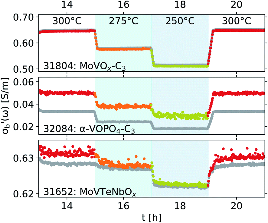 | ||
Fig. 11 Comparison of conductivity traces  obtained as a function of time with three representative samples at three temperatures. Data processed with the TM210 mode used as an internal standard (colours), and with a constant Q0 = 3956 ± 10 (gray) for comparison. obtained as a function of time with three representative samples at three temperatures. Data processed with the TM210 mode used as an internal standard (colours), and with a constant Q0 = 3956 ± 10 (gray) for comparison. | ||
The use of the internal standard allows for an increased instrument uptime, as it is sufficient to measure the properties of the empty cavity (Q0, f0) at a monthly or lower frequency as opposed to the weekly or higher frequency used previously.8 Additionally, the standard parameters for the operation of the network analyser were adjusted to follow the Handbook procedure,6i.e. 20001 points are recorded in each sweep between 7.1 and 7.4 GHz, using a filter bandwidth of 10 kHz, and each datapoint is calculated from the average of 10 sweeps. This approach reduces noise by higher averaging (10 instead of 3 in ref. 8) and increases time-resolution (∼1 min per datapoint instead of ∼3 min in ref. 8). In practical terms, the automation of the instrument allowed for an operando investigation of 27 samples based on pre-defined protocols over a 46 days period. The data collection itself spanned 72% of the total hours in this period, excluding instrument calibration, maintenance and sample preparation, but including nights and weekends, with the instrument operated by a single operator.
3.2 Modularity: comparing algorithms
The modular nature of the yadg software allows for a facile development and a quick and comparative analysis of data using different algorithms. An example is shown in Fig. 12, where the same Γ(f) raw data (measured using the 31804 MoVOx–C3 sample) are processed by yadg to obtain Q0, Qs, f0, and fs using three different algorithms: Kajfez's circle fitting algorithm (colours),14 an algorithm using Lorentzian functions which are fitted to log(|Γ(f)|) (blue), and a naive fit which approximates Q from the full width at half minimum (FWHM) of |Γ(f)| (gray). The qualitative aspects of the plot, i.e. the temperature dependence of are well reproduced by all three algorithms. The absolute
  is reproduced to within a scaling constant, which can be lumped into the fitted parameter C in eqn (4) and (5). However, the circle fitting algorithm is comparably fast (∼1.5 s per trace with 20001 points, including disk I/O) and the most robust of the three, and results in data with the least amount of noise; it is therefore recommended by default. By comparison, the naive algorithm is very noisy due to the comparatively low number of points in each Γ(f) trace.
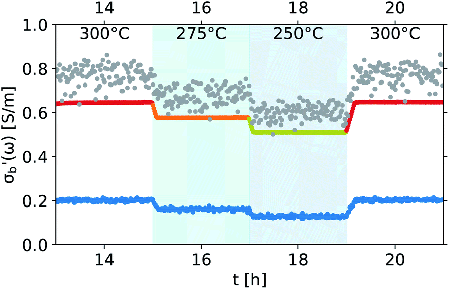 | ||
Fig. 12 Comparison of conductivity traces  of the 31804 MoVOx–C3 sample calculated from Q and f values obtained from Γ(f) with Kajfez's circle fitting algorithm (colours),14 a Lorentzian function model (blue), or naive FWHM algorithm (gray). of the 31804 MoVOx–C3 sample calculated from Q and f values obtained from Γ(f) with Kajfez's circle fitting algorithm (colours),14 a Lorentzian function model (blue), or naive FWHM algorithm (gray). | ||
3.3 Experimental uncertainties: robust cross-sample comparisons
The reproducible and automated protocols as well as the uncertainty propagation performed throughout the analysis allow for a statistically supported discrimination between materials and/or samples. An example is shown in Fig. 13, where two V2O5 samples with a different pre-treatment history (a sample activated in propane, 31846 V2O5–C3 (orange), and its parent sample, 31034 V2O5 (blue)) were studied using the Handbook protocol in the MCPT set-up. At a first glance, panel A shows a significant difference in the properties of the two samples, both in the conductivity (dashed) as well as in conversion (solid). However, as shown in panel B, the selectivity as a function of conversion of the two catalysts is essentially identical, and the differences in conversion in panel A can be explained by different packing density of the samples in the reactor. More importantly, as shown in panel C, the error bars of the reference conductivities (measured at 225 °C in lean air during step 1 of the Handbook protocol, see Fig. 9) of the two samples overlap (0.84 ± 0.36 S m−1 and 0.54 ± 0.15 S m−1), meaning the absolute values of the conductivities when comparing the two experiments are statistically equivalent. Derived properties of the two samples, such as the activation energy of mass-normalized conversion (EA(X/m); 66 ± 15 kJ mol−1 and 60 ± 5 kJ mol−1) as well as the activation energy of conductivity (EA(σ); 8.03 ± 0.04 kJ mol−1 and 8.68 ± 0.09 kJ mol−1) are also in a good agreement, confirming that based on the shown data, the behaviour of the two samples is indistinguishable.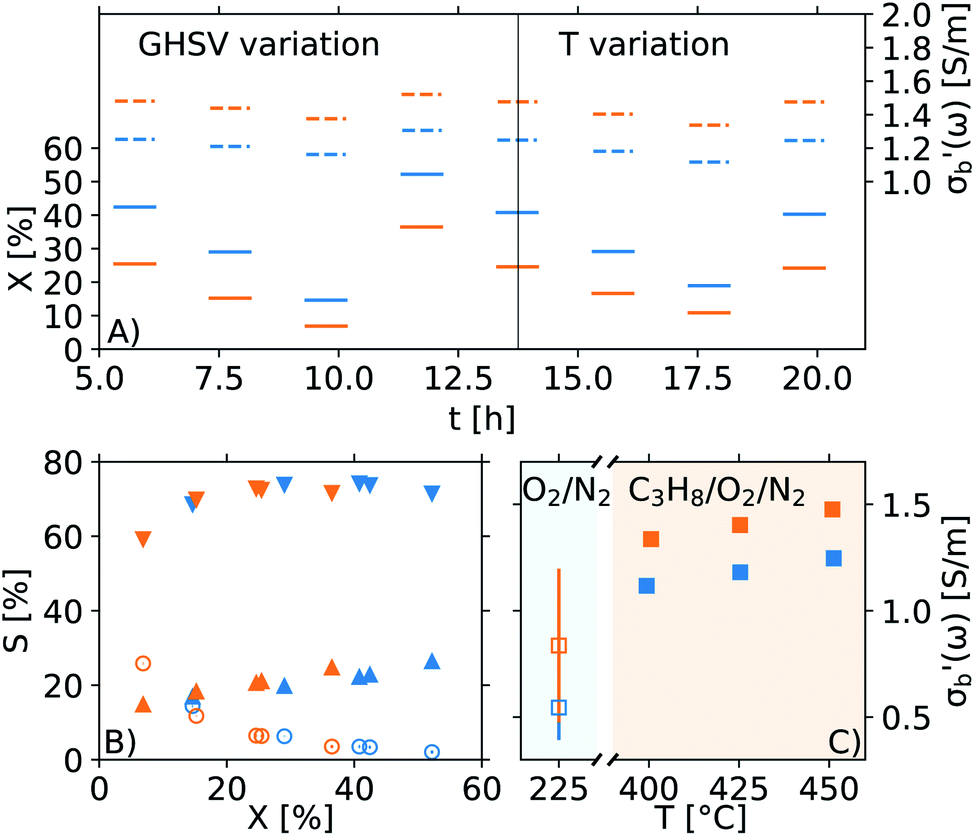 | ||
| Fig. 13 Operando MCPT investigation of two V2O5 samples using the Handbook protocol. A sample activated in propane (31846 V2O5–C3, orange) is compared to its non-activated precursor (31034 V2O5, blue): (A) steps 2–9 of the Handbook protocol, including GHSV variation and T variation; (B) selectivity to C3H6 (○), CO (▽), and CO2 (△) as a function of conversion; (C) conductivity as a function of feed composition and temperature. | ||
The availability of error estimates also aids with data analysis, and provides trust in the absolute values of  Previous reproduction studies using a single batch of vanadium pyrophospate report
  values spanning a factor of 3, depending on the ω and other parameters used.8 Further analysis of this data is hindered by the lack of error estimates in quantities such as catalyst mass (m), sample volume (Vs), or the properties of the empty cavity (f0 and Q0) during each reproduction. A set of new measurements, performed using three fresh aliquots from a single batch of three different materials, are shown in Fig. 14. The results for the three repeats shown in panels A and B using 31848 β-VOPO4–C3 and 31034 V2O5, respectively, are in an excellent agreement with each other, despite the slightly different ranges of conversion covered by each repeat. Note that this degree of reproducibility is achieved with weakly conducting samples (σr of 31848 β-VOPO4–C3 is ∼ 2 × 10⁻² S m−1) as well as for more conductive samples (σr of 31034 V2O5 is ∼ 2 S m−1). An example of a strong conversion dependence is shown in panel C with 31180 LaMn0.80Cu0.20O3: the orange and green repeats cover the same conversion range and nearly identical results are obtained (the points of the two series overlap in the upper panel of Fig. 14C); the red series has been carried out with ∼2× the catalytic mass packed into a similar volume, achieving nearly double the conversion. The red series suffers from significant mass transport issues, confirmed by the slope of conversion as a function of residence time (ΔX(τ)/X), which achieves only 40% of the ideal value.
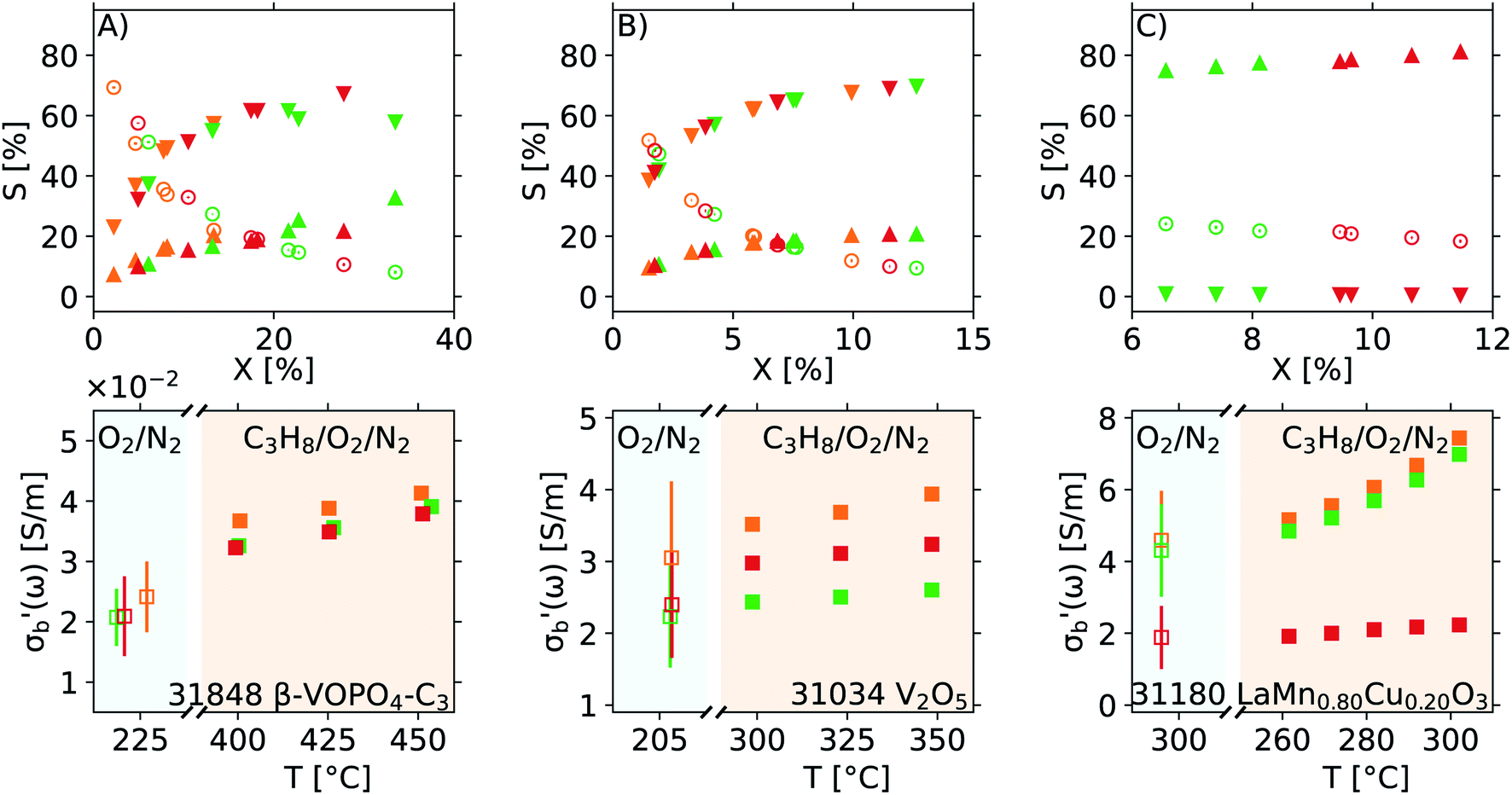 | ||
Fig. 14 Reproduction runs with three sets of samples: (A) 31848 β-VOPO4–C3 investigated using the Handbook protocol; (B) 31034 V2O5 investigated using a development version of the Handbook protocol; and (C) 31180 LaMn0.80Cu0.20O3 investigated using the perovskite protocol. Top panels show selectivity to C3H6 (○), CO (▽) and CO2 (△) as a function of conversion. Bottom panels show the reference conductivity with error bars, and temperature dependence of the conductivity under operating conditions. Note that the error bars for the S/X plots and  points in feed are too small to be visible, indicating the changes in the observed quantities are statistically significant. points in feed are too small to be visible, indicating the changes in the observed quantities are statistically significant. | ||
3.4 Increased resolution: analysis of transients possible
As the acquisition time has been significantly reduced and discontinuities in the conductivity data are avoided, the method is suitable for a transient analysis of samples. An example is shown in Fig. 15, showing the MCPT analysis of a 30624 LaMn0.65Cu0.35O3 sample using the perovskite protocol. We note that the conversion (Xp(C3H8), blue squares) reaches a steady state at every condition, however the conductivity ( top panel) shows a significant upwards drift throughout the experiment (0.33 S m−1 over the course of 30 h). This can be attributed to the desorption of CO2 by oxidation of the carbon-containing impurities on the surface, as shown by the non-zero mol fraction of CO2 in the outlet stream (black triangles) even before the catalyst is exposed to the propane feed. This is consistent with the n-type semiconducting behaviour of this sample: as the adsorbed carbon is removed from the surface by oxygen, the surface of the material is reduced, further filling the conduction band and leading to an increase in σ in n-type semiconductors. The sensitivity of the electrical conductivity to the red-ox behaviour of the system is shown to be significantly higher than the sensitivity of the catalytic conversion. Our testing shows that a quantitative analysis of transient effects on σ in the MCPT instrument is feasible with ∼5 s resolution by simply reducing the amount of averaged scans per datapoint from 10 to 1. A finer time-resolution may be achieved by increasing the filter bandwidth from 10 kHz, potentially sacrificing instrument sensitivity.
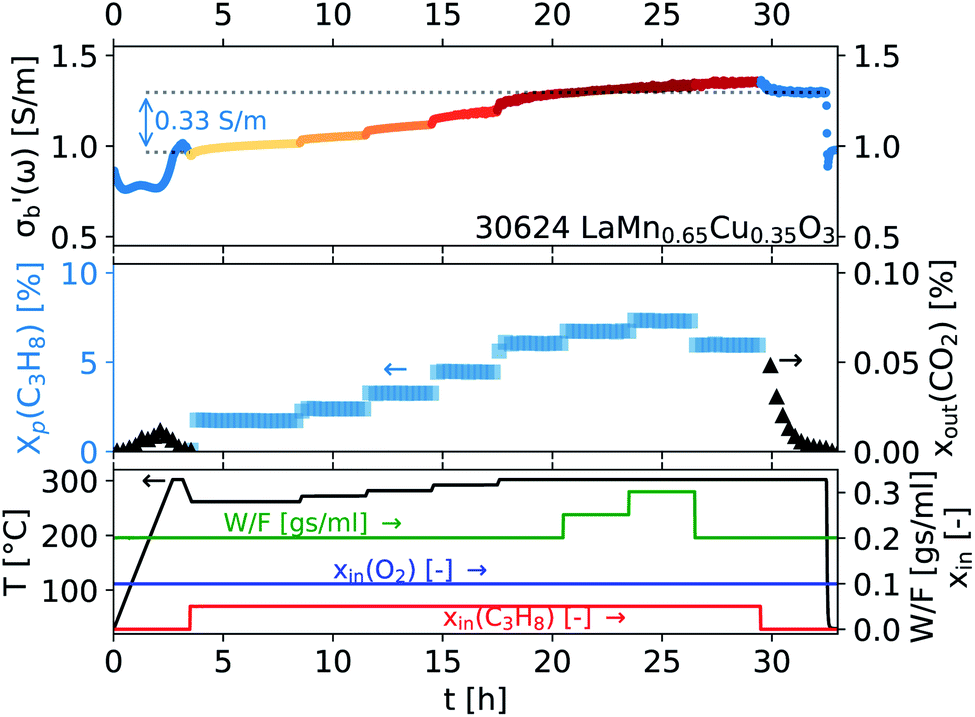 | ||
| Fig. 15 A time-resolved plot of a MCPT experiment using the perovskite protocol. Electrical conductivity (top panel), conversion of propane and outlet molar fraction of CO2 (middle panel), and the temperature, inlet molar fractions of propane and O2, and the catalyst weight over gas flow ratio (bottom panel) are plotted from recorded instrument data within the datagram directly. | ||
3.5 Reproducibility: pathway towards big data
The operando data obtained for all samples studied with the Handbook and perovskite protocols are presented in Tables S1 and S2 in the ESI.† The overall dataset is summarized in Fig. 16, displaying the broad ranges of selectivity and conductivity of the catalysts. While no obvious trend can be deduced from Fig. 16, a machine learning-driven analysis of a subset of data comprising the vanadium containing catalysts (red) revealed a link between conductivity and selectivity of the materials.10 The availability of well annotated operando data, including any “negative results” as shown in Fig. 16, is therefore a key prerequisite for modern, non-linear data-scientific analysis.22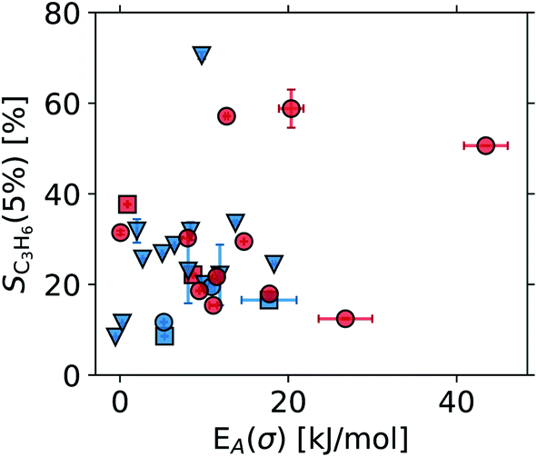 | ||
| Fig. 16 Diversity in the dataset, illustrated via plot of selectivity to propylene at 5% conversion against the activation energy of conductivity. Colours show perovskites (blue) and all other samples (red). Symbols indicate whether the sample was activated in propane prior to the MCPT study (○), or not (□); in both cases the sample was investigated using the Handbook protocol. Additionally, perovskites investigated using the perovskite protocol are included for comparison (▽). | ||
When the operando MCPT results are combined with elemental composition data obtained from X-ray fluorescence and inductively coupled plasma optical emission spectroscopy, an exploratory analysis using a facet–grid plot30 of all observables can quickly reveal trends such as that shown in Fig. 17. Here, two series of copper-doped lanthanide manganates were investigated using the perovskite protocol, and a switch in the semiconducting behaviour from n-type to p-type was observed at Cu substitution levels between 35% and 40% of the total B-sites in the perovskite. The switch in the semiconducting behaviour can be attributed to an increase in MnIV+ centres in the perovskite lattice, which are required to balance the excess charge upon substitution of MnIII+ by CuII+. Cu-substitution therefore introduces holes into the d-band of the perovskite,31 which become the dominant charge carrier above ∼35 at% Cu. The reproducible nature of the automated experiments and the data storage using common formats allows for a systematic analysis in a less diverse set of samples with little effort.
 | ||
| Fig. 17 Semi-conducting behaviour of lanthanide manganates (ABO3 formula). Change in the conductivity as a function of equivalence ratio is plotted against Cu-substitution of Mn at the B-site of the perovskite. The element occupying the A-site is indicated by the symbols: lanthanum (green ▽) or praseodymium (brown △). | ||
4 Summary and outlook
The digitalization of catalysis is an important,4 but long-term goal,2 which is likely to be achieved by iterative development of processes6 rather than a step change. In the present work, we document our efforts in the digitization of data obtained from an operando instrument by automation, and standardised data processing according to FAIR principles. In order to allow for an informed transition towards digital catalysis, we share the design principles, reasoning, and justifications behind the choices in the automation process that we found important during the development of our instrument, from the operator's point of view.This work details the practical implementation of sample protocols, such as the Handbook for Catalysis,6 in an operando study of catalytic samples. We show that by transitioning towards an automated operation of the MCPT set-up, we were able to increase the quality, reproducibility, diversity, and confidence in the obtained data without sacrificing throughput. The increased confidence in the measured conductivity data has implications for the further development of sample protocols: determining a steady state of the system from the catalytic conversion and selectivity alone may not be sufficient, and is in fact impossible under the inert conditions chosen as a reference. Further work is also indicated in aspects of electronic data integration, both before and during the experiment. In fact, data processing routines may be tied back into the instrument control system and provide information about steady state in a closed feedback loop. Another shortcoming of the presented data processing pipeline is its specificity for the MCPT instrument. By tailoring the software to the hardware we were able to develop the toolchain much faster, at the cost of generality and code quality. We are working on further versions of the software, making the toolchain more general, and portable to other instruments.
Finally, we include two self-consistent datasets describing the behaviour of operando electronic conductivity of metal oxide catalysts in propane oxidation. To our best knowledge, these are the first catalytic datasets that include the operando electronic conductivity of the system and conform to the FAIR data principles. A subset of one of the datasets has already been analysed using novel, data-scientific methods,10 and we hope both datasets will be of direct interest to the catalytic community, e.g. as benchmarks.3 Additionally, we hope that our datasets, as well as the processes and tools developed as part of this work, may inform the design of data repositories and infrastructure2 and help with achieving the goals of digital catalysis4 and open science.
Data availability
• The datagrams and parameter files as well as the Jupyter notebooks used to create the figures in this manuscript are archived on Zenodo under https://doi.org/10.5281/zenodo.5011202. The archive is Binder-ready.• A Jupyter notebook containing instruction on installing yadg, as well as its execution to process schema into datagrams, is available on Zenodo under https://doi.org/10.5281/zenodo.5895962. The archive is Binder-ready.
• All processed data (the datagrams and the schema files used to create them, as well as the parameter files) and raw instrument data (instrument logs, VNA logs, chromatograms and run protocols) are available on Zenodo under https://doi.org/10.5281/zenodo.5008960, https://doi.org/10.5281/zenodo.5010992, and https://doi.org/10.5281/zenodo.4980210.
• The calibration files required to process the raw data files contained in the above archives are available on Zenodo under https://doi.org/10.5281/zenodo.5894835.
• The open-source MCPT toolkit including the yadg tool as well as the dg2png and dg2json scripts is available on Zenodo at https://doi.org/10.5281/zenodo.5894823. The code is also available on Github under dgbowl/yadg. The data in this work were processed using version yadg-3.1.0 or earlier.
• The LabView VI developed for the automation of the MCPT instrument is available on Zenodo under https://doi.org/10.5281/zenodo.5571298. Further information available from the authors on request.
Conflicts of interest
There are no conflicts to declare.Acknowledgements
This work was conducted in the framework of the BasCat collaboration among BASF SE, Technical University Berlin, Fritz Haber Institute of the Max Planck Society, and the cluster of excellence “Unified Concepts in Catalysis” (UniCat, see http://www.unicat.tu-berlin.de). The authors would like to thank Stephen Lohr and Sven Richter for the synthesis of vanadium samples, Rania Hanna for sample pressing and sieving, Dr Pierre Kube for sample activation, Tobias Lewerenz for the technical drawings, Dr Nicolai Groβe for numerous consultations, Dr Olaf Timpe for XRF and ICP-OES analysis, Dr Frank Girgsdies for XRD analysis, and Dr Frank Rosowski. P. K. would like to thank the Forrest Research Foundation for funding. E. H. W. would like to thank the IMPRS (International Max Planck Research School) “Functional Interfaces in Physics and Chemistry” for funding and support.References
- R. Schlögl, Catalysis 4.0, ChemCatChem, 2017, 9, 533–541 CrossRef.
- P. S. F. Mendes, S. Siradze, L. Pirro and J. W. Thybaut, Open data in catalysis: From today's big picture to the future of small data, ChemCatChem, 2021, 13, 836–850 CrossRef CAS.
- T. Bligaard, R. M. Bullock, C. T. Campbell, J. G. Chen, B. C. Gates, R. J. Gorte, C. W. Jones, W. D. Jones, J. R. Kitchin and S. L. Scott, Toward benchmarking in catalysis science: Best practices, challenges, and opportunities, ACS Catal., 2016, 6, 2590–2602 CrossRef CAS.
- D. Demtröder, O. Deutschmann, B. Eck, R. Franke, R. Gläser, L. Goosen, J. D. Grunwaldt, R. Krähnert, U. Kragl, W. Leitner, G. Mestl, K. Reuter, F. Rosowski, A. Schäfer, M. Scheffler, R. Schlögl, F. Schüth, S. A. Schunk, F. Studt, K. Wagemann, P. Wasserscheid, C. Wöll, and D. Wolf, The digitalization of catalysis-related sciences, whitepaper, German Catalysis Society (GeCatS), Mar. 2019 Search PubMed.
- NCCR Catalysis: Our approach, https://www.nccr-catalysis.ch/research/approach/, June 2021 Search PubMed.
- A. Trunschke, G. Bellini, M. Boniface, S. J. Carey, J. Dong, E. Erdem, L. Foppa, W. Frandsen, M. Geske, L. M. Ghiringhelli, F. Girgsdies, R. Hanna, M. Hashagen, M. Hävecker, G. Huff, A. Knop-Gericke, G. Koch, P. Kraus, J. Kröhnert, P. Kube, S. Lohr, T. Lunkenbein, L. Masliuk, R. Naumann d'Alnoncourt, T. Omojola, C. Pratsch, S. Richter, C. Rohner, F. Rosowski, F. Rüther, M. Scheffler, R. Schlögl, A. Tarasov, D. Teschner, O. Timpe, P. Trunschke, Y. Wang and S. Wrabetz, Towards experimental handbooks in catalysis, Top. Catal., 2020, 63, 1683–1699 CrossRef CAS.
- M. Eichelbaum, R. Stößer, A. Karpov, C.-K. Dobner, F. Rosowski, A. Trunschke and R. Schlögl, The microwave cavity perturbation technique for contact-free and in situ electrical conductivity measurements in catalysis and materials science, Phys. Chem. Chem. Phys., 2012, 14(3), 1302–1312 RSC.
- A. M. Wernbacher, M. Eichelbaum, T. Risse, S. Cap, A. Trunschke and R. Schlögl, Operando electrical conductivity and complex permittivity study on vanadia oxidation catalysts, J. Phys. Chem. C, 2019, 123, 8005–8017 CrossRef CAS.
- M. Eichelbaum, M. Hävecker, C. Heine, A. M. Wernbacher, F. Rosowski, A. Trunschke and R. Schlögl, The electronic factor in alkane oxidation catalysis, Angew. Chem., Int. Ed., 2015, 54, 2922–2926 CrossRef CAS PubMed.
- L. Foppa, L. M. Ghiringhelli, F. Girgsdies, M. Hashagen, P. Kube, M. Hävecker, S. J. Carey, A. Tarasov, P. Kraus, F. Rosowski, R. Schlögl, A. Trunschke and M. Scheffler, Materials genes of heterogeneous catalysis from clean experiments and artificial intelligence, MRS Bull., 2021, 46, 1016–1026 CrossRef CAS PubMed.
- M. Heenemann, Charge transfer in catalysis studied by in situ microwave cavity perturbation techniques, PhD thesis, Technische Universität Berlin, Berlin, 2017.
- C. Heine, F. Girgsdies, A. Trunschke, R. Schlögl and M. Eichelbaum, The model oxidation catalyst α-V2O5: insights from contactless in situ microwave permittivity and conductivity measurements, Appl. Phys. A, 2013, 112, 289–296 CrossRef CAS.
- D. Slocombe, The electrical properties of transparent conducting oxide composites. PhD thesis, Cardiff University, Cardiff, 2012.
- D. Kajfez, Linear fractional curve fitting for measurement of high Q factors, IEEE Trans. Microwave Theory Techn., July 1994, 42, 1149–1153 Search PubMed.
- H. Looyenga, Dielectric constants of heterogeneous mixtures, Physica, 1965, 31, 401–406 CrossRef CAS.
- D. C. Dube, Study of Landau-Lifshitz-Looyenga’s formula for dielectric correlation between powder and bulk, J. Phys. D: Appl. Phys., 1970, 3, 1648–1652 CrossRef CAS.
- C. D. Hawker, Nonanalytic laboratory automation: A quarter century of progress, Clin. Chem., 2017, 63, 1074–1082 CrossRef CAS PubMed.
- J. A. Selekman, J. Qiu, K. Tran, J. Stevens, V. Rosso, E. Simmons, Y. Xiao and J. Janey, High-throughput automation in chemical process development, Annu. Rev. Chem. Biomol. Eng., 2017, 8, 525–547 CrossRef PubMed.
- D. A. Armbruster, D. R. Overcash and J. Reyes, Clinical chemistry laboratory automation in the 21st century - Amat victoria curam (Victory loves careful preparation), Clin. Biochem. Rev., 2014, 35(3), 143–153 Search PubMed.
- S. M. Mennen, C. Alhambra, C. L. Allen, M. Barberis, S. Berritt, T. A. Brandt, A. D. Campbell, J. Castañón, A. H. Cherney, M. Christensen, D. B. Damon, J. Eugenio de Diego, S. García-Cerrada, P. García-Losada, R. Haro, J. Janey, D. C. Leitch, L. Li, F. Liu, P. C. Lobben, D. W. C. MacMillan, J. Magano, E. McInturff, S. Monfette, R. J. Post, D. Schultz, B. J. Sitter, J. M. Stevens, I. I. Strambeanu, J. Twilton, K. Wang and M. A. Zajac, The evolution of high-throughput experimentation in pharmaceutical development and perspectives on the future, Org. Process Res. Dev., 2019, 23, 1213–1242 CrossRef CAS.
- S. Steiner, J. Wolf, S. Glatzel, A. Andreou, J. M. Granda, G. Keenan, T. Hinkley, G. Aragon-Camarasa, P. J. Kitson, D. Angelone and L. Cronin, Organic synthesis in a modular robotic system driven by a chemical programming language, Science, 2019, 363, eaav2211 CrossRef CAS PubMed.
- A. G. Godfrey, S. G. Michael, G. S. Sittampalam and G. Zahoránszky-Köhalmi, A perspective on innovating the chemistry lab bench, Front. Robot. AI, 2020, 7, 24 CrossRef PubMed.
- G. Lippi and G. Da Rin, Advantages and limitations of total laboratory automation: a personal overview, Clin. Chem. Lab. Med., 2019, 57, 802–811 CrossRef CAS PubMed.
- P. Orange, J. Willmot, and W. Fazackerley, Good automation practices in the laboratory, Pharmaceutical Technology’s In the Lab eNewsletter, vol. 15, pp. 44–45, June 2020 Search PubMed.
- D. G. A. Smith, D. Altarawy, L. A. Burns, M. Welborn, L. N. Naden, L. Ward, S. Ellis, B. P. Pritchard and T. D. Crawford, The MolSSI QCArchive project: An open-source platform to compute, organize, and share quantum chemistry data, WIREs Comput. Mol. Sci., 2021, 11(2), e1491 CAS.
- A. M. Wernbacher, P. Kube, M. Hävecker, R. Schlögl and A. Trunschke, Electronic and dielectric properties of MoV-oxide (M1 ohase) under alkane oxidation conditions, J. Phys. Chem. C, 2019, 123, 13269–13282 CrossRef CAS.
- A. Trunschke, J. Noack, S. Trojanov, F. Girgsdies, T. Lunkenbein, V. Pfeifer, M. Hävecker, P. Kube, C. Sprung, F. Rosowski and R. Schlögl, The impact of the bulk structure on surface dynamics of complex Mo–V-based oxide catalysts, ACS Catal., 2017, 7, 3061–3071 CrossRef CAS.
- M. Sanchez Sanchez, F. Girgsdies, M. Jastak, P. Kube, R. Schlögl and A. Trunschke, Aiding the self-assembly of supramolecular polyoxometalates under hydrothermal conditions to give precursors of complex functional oxides, Angew. Chem., Int. Ed., 2012, 51, 7194–7197 CrossRef CAS PubMed.
- M. P. Pechini, Method of preparing lead and alkaline earth titanates and niobates and coating method using the same to form a capacitor, July 1967 Search PubMed.
- M. Waskom, Seaborne: statistical data visualization, J. Open Source Softw., 2021, 6, 3021 CrossRef.
- T. Arakawa, H. Kurachi and J. Shiokawa, Physicochemical properties of rare earth perovskite oxides used as gas sensor material, J. Mater. Sci., 1985, 20, 1207–1210 CrossRef CAS.
Footnote |
| † Electronic supplementary information (ESI) available. See DOI: 10.1039/d1dd00029b |
| This journal is © The Royal Society of Chemistry 2022 |