
 Open Access Article
 This Open Access Article is licensed under a
 Creative Commons Attribution 3.0 Unported Licence
The surface site interaction point approach to non-covalent interactions†
Maria Chiara
Storer
 and
Christopher A.
Hunter
*
and
Christopher A.
Hunter
*
Yusuf Hamied Department of Chemistry, University of Cambridge, Lensfield Road, Cambridge, CB2 1EW, UK. E-mail: herchelsmith.orgchem@ch.cam.ac.uk
First published on 22nd November 2022
Abstract
The functional properties of molecular systems are generally determined by the sum of many weak non-covalent interactions, and therefore methods for predicting the relative magnitudes of these interactions is fundamental to understanding the relationship between function and structure in chemistry, biology and materials science. This review focuses on the Surface Site Interaction Point (SSIP) approach which describes molecules as a set of points that capture the properties of all possible non-covalent interactions that the molecule might make with another molecule. The first half of the review focuses on the empirical non-covalent interaction parameters, α and β, and provides simple rules of thumb to estimate free energy changes for interactions between different types of functional group. These parameters have been used to have been used to establish a quantitative understanding of the role of solvent in solution phase equilibria, and to describe non-covalent interactions at the interface between macroscopic surfaces as well as in the solid state. The second half of the review focuses on a computational approach for obtaining SSIPs and applications in multi-component systems where many different interactions compete. Ab initio calculation of the Molecular Electrostatic Potential (MEP) surface is used to derive an SSIP description of a molecule, where each SSIP is assigned a value equivalent to the corresponding empirical parameter, α or β. By considering the free energies of all possible pairing interactions between all SSIPs in a molecular ensemble, it is possible to calculate the speciation of all intermolecular interactions and hence predict thermodynamic properties using the SSIMPLE algorithm. SSIPs have been used to describe both the solution phase and the solid state and provide accurate predictions of partition coefficients, solvent effects on association constants for formation of intermolecular complexes, and the probability of cocrystal formation. SSIPs represent a simple and intuitive tool for describing the relationship between chemical structure and non-covalent interactions with sufficient accuracy to understand and predict the properties of complex molecular ensembles without the need for computationally expensive simulations.
 Maria Chiara Storer | Maria Chiara Storer received her BA and MSc degrees in Natural Sciences at the University of Cambridge. She has been a PhD student of Professor Christopher Hunter at the Yusuf Hamied Department of Chemistry at the University of Cambridge since 2019. The focus of her doctoral research is the quantitative prediction of non-covalent interactions and in particular extending the scope of the Surface Site Interaction Point model. |
 Christopher A. Hunter | Chris Hunter was educated at the University of Cambridge. He was a lecturer at the University of Otago in New Zealand till 1991, when he moved to the University of Sheffield. He was promoted to a chair in 1997, and in 2014, he took up the Herchel Smith Professorship of Organic Chemistry at the University of Cambridge. In 2008, he was elected a Fellow of the Royal Society, and he is an Honorary Member of the Royal Irish Academy. His research focusses on the chemistry of non-covalent interactions, combining physical organic chemistry, computational modelling and synthetic supramolecular chemistry. |
1 Introduction
The functional properties of most organic molecules are determined by the way in which they interact with other molecules. Non-covalent interactions determine the organisation of organic molecules in materials, the folding and self-organisation of biomolecules, the formation of intermolecular complexes and supramolecular assemblies, as well as partitioning and solubility of small molecules.1–3 They also play an important role in many catalytic processes.4,5 Prediction of these properties is challenging, because they involve the interplay of multiple relatively weak interactions between different molecules, including the solvent. Empirical scales of non-covalent interaction parameters have been developed to characterise the relationship between the chemical structures of the functional groups involved and the interaction energies.6,7Ab initio calculations have been used to provide insight into the forces that govern different types of non-covalent interaction, and molecular dynamics approaches are being developed to calculate free energy changes for solution phase processes.8,9 We have been working on a method that attempts to combine insights from experiment and theory to develop simple tools capable of describing the relationship between chemical structure and non-covalent interactions with sufficient accuracy to understand and predict the properties of complex molecular ensembles.The basis of the approach is the description of a molecule as a set of Surface Site Interaction Points (SSIP) that capture the properties of all possible non-covalent interactions that the molecule might make with another molecule.10 Each SSIP represents an area of approximately 9 Å2 on the van der Waals surface, which corresponds to the footprint of a single hydrogen bond (H-bond).10 SSIPs can exist in one of two states, either non-bonded or paired with an SSIP from another molecule, and interactions between SSIPs are mutually exclusive. The non-polar interaction between two SSIPs is described by a constant van der Waals energy, but SSIPs also have polarity, so there is an additional polar contribution to the interaction energy when a positive SSIP interacts with a negative SSIP. Positive SSIPs represent regions of local positive electrostatic potential, associated with H-bond donors or σ-holes, and interactions at these sites are quantified by the non-covalent interaction parameter α. Negative SSIPs represent regions of local negative electrostatic potential, associated with lone pair H-bond acceptor sites or π-electron density, and interactions at these sites are quantified by the non-covalent interaction parameter β.
Fig. 1 shows the SSIP representation of two simple molecules.11 Methanol is described by six SSIPs: the two negative SSIPs (red) represent the lone pair H-bond acceptor sites on the oxygen; the large positive SSIP (blue) represents the H-bond donor site on the hydroxyl group; and the small positive SSIPs represent the less polar CH groups. Pyridine is described by eight SSIPs: the large negative SSIP represents the H-bond acceptor site at the nitrogen lone pair; there is one small negative SSIP on each face of the ring, representing sites of interaction with the π-electron density; and five positive SSIPs represent the CH groups. These SSIPs allow prediction of the energies of non-covalent interactions with these molecules. For example in a mixture of pyridine and methanol, the most favourable interaction is between the negative SSIP that represents the lone pair of the pyridine nitrogen, which has the largest β value, and the positive SSIP that represents the methanol hydroxyl proton, which has the largest α value. The structure of the resulting H-bonded complex is illustrated in Fig. 1, and the polar contribution to the interaction energy is quantified by the product of the non-covalent interaction parameters that describe the two SSIPs, −(α × β).
 | ||
| Fig. 1 The Surface Site Interaction Point (SSIP) description of methanol and pyridine shown as a set of spheres on the van der Waals surface. Negative SSIPs (red) are described by the non-covalent interaction parameter β, positive SSIPs (blue) are described by the non-covalent interaction parameter α, and the size of each sphere is proportional to the value of α or β. The H-bonded complex shown is described as a contact between the SSIP that represents the pyridine lone pair H-bond acceptor and the SSIP that represents the methanol hydroxyl H-bond donor, and the interaction energy is quantified by multiplying the corresponding non-covalent interaction parameters, −(α × β). | ||
Here we provide an overview of the development of the SSIP approach and discuss applications to understanding the thermodynamic properties of intermolecular complexes and solvation free energies. The review is broadly divided into two parts. The first half focuses on the empirical non-covalent interaction parameters, α and β, which have been developed to describe the properties of different functional groups and form the basis for describing the interaction properties of SSIPs. These empirical parameters have been used to establish a quantitative understanding of the role of solvent in solution phase equilibria, and to describe non-covalent interactions at the interface between macroscopic surfaces as well as in the solid state. The second half of the review focuses on a computational approach to predicting the properties of molecular ensembles using SSIPs. Ab initio calculation of the Molecular Electrostatic Potential (MEP) surface is used to derive an SSIP description of a molecule, where each SSIP is assigned a non-covalent interaction parameter, which is equivalent to the corresponding empirical parameter, α or β. By considering the free energies of all possible pairing interactions between all SSIPs in a molecular ensemble, it is possible to calculate the speciation of all intermolecular interactions and hence predict thermodynamic properties. Applications of this approach to both the solution phase and the solid state are discussed, including methods that have been developed for virtual cocrystal screening, prediction of partition coefficients and solvent effects on association constants for formation of intermolecular complexes.
2 Empirical non-covalent interaction parameters
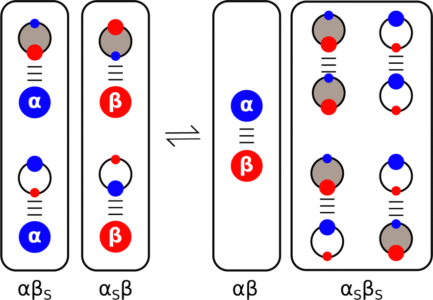
Solvatochromic dyes have been used to probe non-covalent interactions between solvents and solutes, and empirical scales have been developed to characterise solvation properties in terms of specific interactions with solutes.12–15 For example, the Taft solvent parameters quantify how strongly a solvent interacts with H-bond acceptor and H-bond donor sites on solutes. The thermodynamic properties of 1![[thin space (1/6-em)]](https://www.rsc.org/images/entities/char_2009.gif) :1 complexes formed in non-polar organic solvents have been used to probe non-covalent interactions between two solutes. IR, NMR and UV-Vis titrations were used to measure association constants (K) for the formation of H-bonded complexes between thousands of different compounds. These experiments provided insight into the H-bonding properties of a wide range of different functional groups, because simple molecules were chosen, so that complexation was dominated by a single H-bonding interaction between two well-defined polar sites. The experimental data were used to establish empirical scales, such as pKHB for H-bond acceptors,16,17 and Abraham developed the approach further with the H-bond donor and acceptor parameters, αH2 and βH2, that can be multiplied together to predict the relative strengths of interactions between different solutes.6 Hunter generalised the application of these parameters to any solvent environment by explicitly including the competition between solute and solvent interactions (Fig. 2).18 The assumption is that the equilibrium is dominated by interactions between the most polar sites on the solute and the most polar sites on the solvent. Therefore the experimentally determined non-covalent interaction parameters that describe the properties of the most polar sites of the two solutes (α and β) and of the solvent (αS and βS) can be used to estimate the free energy change associated with the exchange of pairwise interactions illustrated in Fig. 2 (eqn (1)).18
:1 complexes formed in non-polar organic solvents have been used to probe non-covalent interactions between two solutes. IR, NMR and UV-Vis titrations were used to measure association constants (K) for the formation of H-bonded complexes between thousands of different compounds. These experiments provided insight into the H-bonding properties of a wide range of different functional groups, because simple molecules were chosen, so that complexation was dominated by a single H-bonding interaction between two well-defined polar sites. The experimental data were used to establish empirical scales, such as pKHB for H-bond acceptors,16,17 and Abraham developed the approach further with the H-bond donor and acceptor parameters, αH2 and βH2, that can be multiplied together to predict the relative strengths of interactions between different solutes.6 Hunter generalised the application of these parameters to any solvent environment by explicitly including the competition between solute and solvent interactions (Fig. 2).18 The assumption is that the equilibrium is dominated by interactions between the most polar sites on the solute and the most polar sites on the solvent. Therefore the experimentally determined non-covalent interaction parameters that describe the properties of the most polar sites of the two solutes (α and β) and of the solvent (αS and βS) can be used to estimate the free energy change associated with the exchange of pairwise interactions illustrated in Fig. 2 (eqn (1)).18| ΔΔG/kJ mol−1 = (αβS + αSβ) − (αβ + αSβS) | (1) |
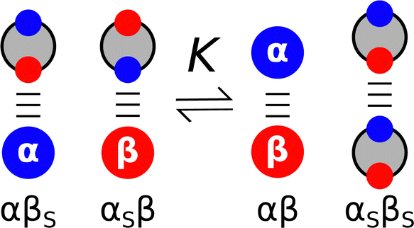 | ||
| Fig. 2 Solvent competition model for complex formation between a H-bond donor (α) and a H-bond acceptor (β) in a solvent, which is described by the H-bond parameters αS and βS. The free energy contribution from pairwise interactions between solutes or solvents is given by the product of the corresponding H-bond parameters. | ||
The value of the association constant for formation of a 1:1 complex (K) is obtained by addition of a constant c, which is related to the entropy changes associated with bimolecular association and desolvation (eqn (2)).
| −RTlnK/kJ mol−1 = − (α − αS)(β − βS) + c | (2) |
The value of c was experimentally determined to be 6 kJ mol−1 in carbon tetrachloride solution, and this value has been shown to provide a good description of a range of different solvents.18–20 The four non-covalent interaction terms in eqn (2) make it clear that the position of equilibrium in Fig. 2 depends on the relative polarities of the solutes and the solvent. The key point is that the solvent is treated in exactly the same way as the solute, and so the non-covalent interaction parameters that have been determined for solutes can be used to describe the same functional groups when they occur in a solvent.18,21,22
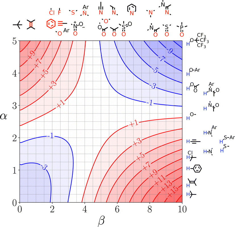
Fig. 3 illustrates the range of values of α and β found for different functional groups. The values of α generally fall in the range 0–5, and the values of β for most functional groups fall in the range 0–10. Variations in the values of the non-covalent interaction parameters can be understood based on the polarity of the atom at the site of interaction. For example, the presence of a nearby electron-withdrawing group would increase the value of α and decrease the value of β. Fig. 3 also includes parameters for anions and cations (red and blue boxes respectively). These parameters can be used in eqn (2) to describe interactions between a neutral solute and a charged solute, but interactions between two charged solutes are beyond the scope of the current treatment, because additional Coulombic interactions come into play. A more complete listing of experimentally determined α and β parameters derived from literature data on the formation of 1:1 complexes is provided in the (ESI†).23–57 Although these parameters were determined from measurements of H-bonded complexes involving polar functional groups, they can be applied to all classes of non-covalent interaction. A H-bond is defined as an attractive interaction between the hydrogen atom of an XH group, in which X is more electronegative than H, and another atom,58 but the non-covalent interaction parameters in Fig. 3 encompass a wider range of functional groups. For example, the α parameter of the iodo compound in Fig. 3 describes a positive σ-hole, which is a region of electron density deficiency located on the surface of the iodine atom on the extension of the carbon–iodine bond axis.59,60 A halogen-bonding interaction between this σ-hole and the lone pair of another compound is described in the same way as a H-bond, i.e. using −(α × β).61 Similarly, different combinations of the functional groups in Fig. 3 can be used to describe any other class of non-covalent interaction, such as aromatic interactions62,63 or weak polar interactions with non-polar functional groups that do not form conventional H-bonds. As will be explained below, the non-covalent interaction parameters illustrated in Fig. 3 are the basis for the SSIP approach, which is used to describe the entire surface of a molecule, rather than single point contacts at the most polar site.
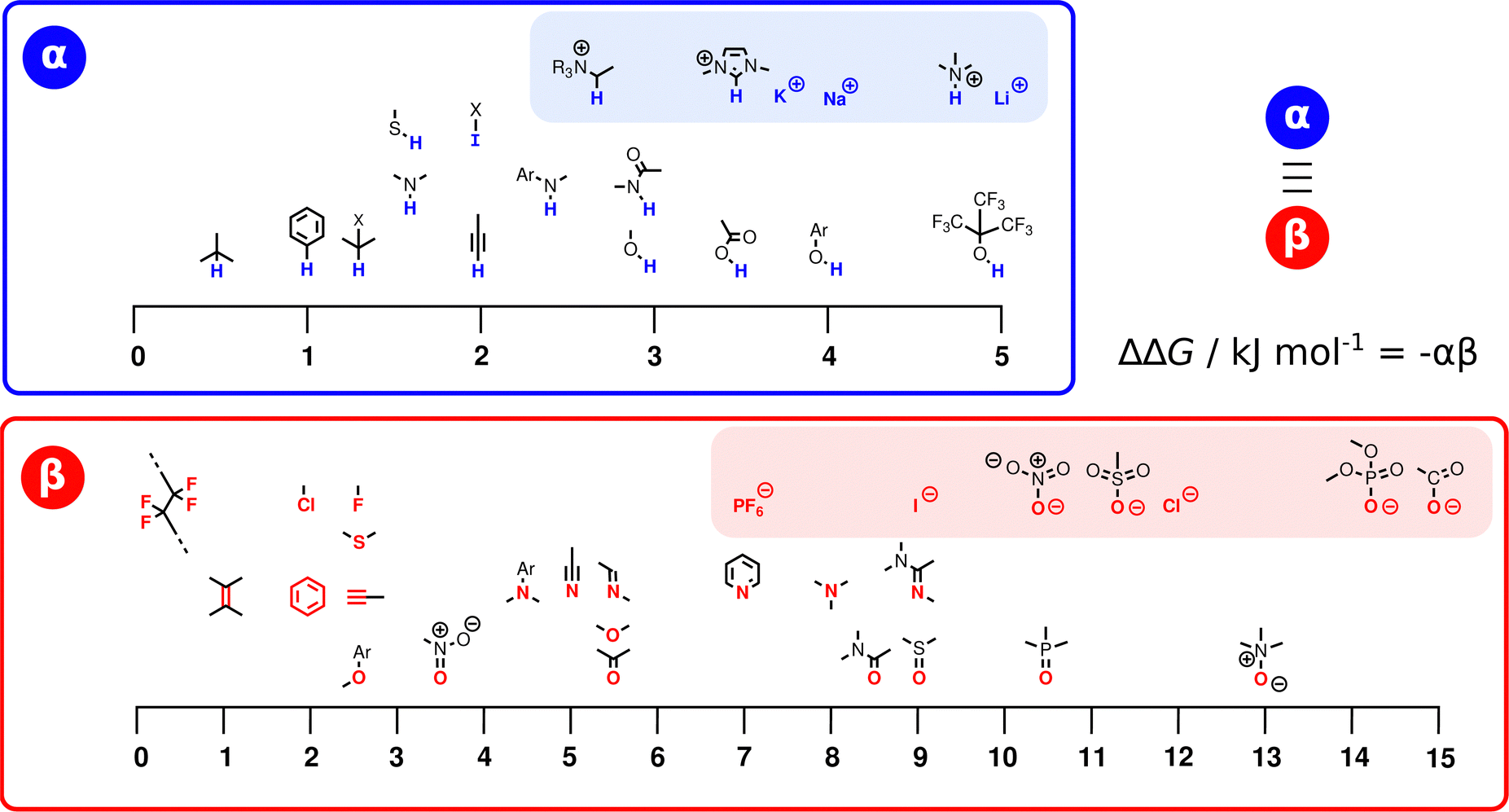 | ||
| Fig. 3 The α and β parameters used to describe non-covalent interactions with different functional groups. The atoms highlighted in blue (α) and red (β) are the atoms involved in the interaction, and ions are separated in shaded boxes. X represents an electron-withdrawing group (see ESI† for complete listing of experimentally determined parameters). | ||
Eqn (2) can be used to obtain a quantitative description of the effects of solvent on the properties of non-covalent interactions. For example, the association constant measured for the 1:1 complex formed between perfluoro-t-butanol and tri-n-butylphosphine oxide decreases by five orders of magnitude when the solvent polarity is increased from benzene to N-methyl formamide, and the values measured in 10 different solvents were accurately predicted by eqn (2) (RMSE in logK = 0.18).19 Similarly, eqn (2) accurately predicted the values of the association constants for 254 different 1:1 complexes, which were experimentally measured in seven different organic solvents (RMSE in logK = 0.32).20
However, when eqn (2) was applied to H-bonded complexes in alcohol solvents, the predicted association constants were more than an order magnitude higher than the values measured experimentally.19 The reasons for this discrepancy, and the properties of alcohol solvents will be discussed in more detail below.
The original H-bond scales were developed by measuring association constants for formation of complexes in non-polar solvents. In effect, these experiments fixed the values of αS and βS in eqn (2) and used association constants for different solute combinations to determine the corresponding α and β parameters. An alternative approach is to use association constants for combinations of solutes with known α and β parameters in eqn (2) to determine values of αS and βS for the solvent. This method has been used to determine empirical non-covalent interaction parameters for non-polar solvents like hydrocarbons and perfluorocarbons.20
2.1 Functional group interaction profiles
The ideas encapsulated in Fig. 2 can be used to construct Functional Group Interaction Profiles (FGIP) that provide maps of the free energy landscape of all possible pairwise functional group interactions in a particular solvent environment.18 The results are illustrated schematically in Fig. 4. An FGIP is a graphical representation of eqn (1) and partitions the functional group interaction space into four quadrants. The solvent parameters αS and βS set the dividing lines, because when α = αS or β = βS, all interactions cancel out, and there is no free energy change associated with the exchange of pairwise interactions between solvent and solutes. The two red quadrants in Fig. 4 identify combination of solutes for which non-covalent interactions are unfavourable, because in these regions, one of the two solute–solvent complexes in Fig. 2 is the most stable of the four possible pairwise interactions. The two blue quadrants identify the combinations of solute for which non-covalent interactions are favourable. In one of these quadrants, the solutes are both more polar than the solvent, so the solute–solute interaction dominates (top right in Fig. 4). In the other blue quadrant, the solutes are both less polar than the solvent, so the solvent–solvent interaction dominates (bottom left in Fig. 4), i.e. this quadrant represents the solvophobic region.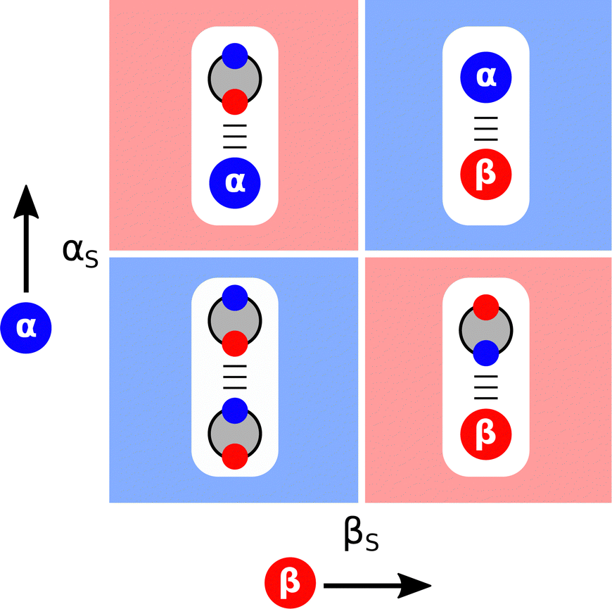 | ||
| Fig. 4 Generalised Functional Group Interaction Profiles (FGIP) which shows the free energy landscape for interaction between two solutes (α and β) in a solvent (αS and βS) as defined by ΔΔG in eqn (1). The blue regions indicate solute combinations that make favourable interactions, and the red regions indicate solute combinations for which interactions are unfavourable. The most stable pairwise interaction that dominates the equilibrium in Fig. 2 is illustrated for each quadrant. | ||
Fig. 5 shows how the non-covalent interaction parameters of common solvents, αS and βS, map onto the FGIP, and Fig. 6 shows how the appearance of the FGIP changes for different types of solvent. Non-polar solvents like hydrocarbons and perfluorocarbons have low values of αS and βS and lie in the bottom left corner of the solvent map in Fig. 5. The corresponding FGIP for cyclohexane shown in Fig. 6(a) is almost completely blue, because the solute–solute interaction always dominates the equilibrium. All interactions between solute functional groups are favourable, which accounts for the poor solvating properties of these solvents.
 | ||
| Fig. 5 Map of the non-covalent interaction parameters that describe the properties of common solvents (αS and βS). Polar interaction sites are highlighted in blue (αS) and red (βS) (see ESI† for complete listing of experimentally determined parameters). | ||
 | ||
| Fig. 6 Functional Group Interaction Profiles (FGIP) showing the free energy landscape for interaction between two solutes (α and β) in (a) a non-polar solvent, cyclohexane, (b) a polar protic solvent, water, (c) a very polar aprotic solvent, DMSO, (d) a moderately polar aprotic solvent, THF, (e) a polar fluorinated solvent, hexafluoroisopropanol, (f) a halogenated solvent, chloroform. The blue regions indicate solute combinations that make favourable interactions, and the red regions indicate solute combinations for which interactions are unfavourable. Where one quadrant dominates the FGIP, the relevant pairwise interaction is illustrated. | ||
Polar protic solvents like water fall in the centre of the solvent map in Fig. 5 and 6(b) shows the corresponding FGIP. The four quadrants of the FGIP are approximately the same size, because the solvent parameters lie in the middle of the solute α and β scales. As a result, solvophobic effects and polar interactions play an equally important role in determining the properties of non-covalent interactions between solutes in water. Other polar protic solvents, like alcohols and carboxylic acids, are not shown in Fig. 5, because they have non-polar functional groups that play a role in solvation of solutes. A treatment for obtaining FGIPs for these more complicated solvents and the consequences for solvophobic region will be discussed later.
Polar aprotic solvents are characterised by low values of αS, but this group of solvents spans a wide range of βS values. The most polar examples, like dimethylsulfoxide (DMSO) and hexamethylphosphoramide (HMPA), are grouped in the bottom left corner of the solvent map in Fig. 5, and the corresponding FGIP is shown in Fig. 6(c). The FGIP for DMSO is almost completely red, because solvation by the solvent H-bond acceptor dominates the equilibrium. Almost all interactions between solute functional groups are unfavourable, which explains why DMSO is such a good solvent. THF is also a polar aprotic solvent, but in this case, the value of βS lies in the middle of the solute β scale. The resulting FGIP shown in Fig. 6(d) is dominated by two quadrants, one in which polar solutes make favourable interactions (blue) and one in which solvation by the solvent H-bond acceptor dominates (red).
Polar fluorinated solvents are grouped in the top left corner of the solvent map in Fig. 5 and constitute a special class of solvents with unique properties. The FGIP for hexafluoroisopropanol (HFIP) shown in Fig. 6(e) is almost completely red, because solvation by the solvent H-bond donor dominates the equilibrium. There is a clear relationship between the FGIPs for DMSO in Fig. 6(c) and HFIP in Fig. 6(e). Both solvents break up almost all solute–solute interactions, but DMSO solvates H-bond acceptors and anions poorly, whereas HFIP solvates H-donors and cations poorly. These selective solvation properties can lead to enhanced rates of chemical reaction in these solvents, if a key reactant is poorly solvated.64–67
Fig. 6(f) shows the FGIP for chloroform. Halogenated solvents have values of βS that are similar to hydrocarbons but the values of αS are significantly higher. As a result, the FGIP is dominated by two quadrants, one in which polar solutes make favourable interactions (blue) and one in which solvation by the solvent CH group dominates (red). Fig. 6 provides a qualitative illustration of the solvation properties of six different classes of solvent, but it is also possible to construct quantitative FGIPs that map the value of ΔΔG for any solute combination in any solvent or solvent mixture. Application of this approach to obtain FGIPs for alcohols and solvent mixtures is discussed in detail below.
2.2 Solvation properties of solvent mixtures
Experiments on the properties of H-bonded complexes in solvent mixtures confirm the validity of treating solvation as a set of competing equilibria between pairwise interactions of solute and solvent molecules.68–72Fig. 7 shows how the solvent competition model can be extended to describe complexation in a mixture of two different solvents. The solute–solute interaction is the same as in Fig. 2, but now the solute–solvent interactions both involve two solvation states, due to the two different complexes that can be formed with the two different solvents, and there are four possible solvent–solvent interactions. The multiple competing equilibria lead to a significant increase in complexity, but the overall behaviour of the system can still be understood based on the relative stability of each of the pairwise interactions shown in Fig. 7. For example, the association constant for the 1:1 complex formed between perfluoro-t-butanol and tri-n-butyl phosphine oxide in mixtures of chloroform and tetrahydrofuran (THF) is an order of magnitude lower than the value measured in either of the pure solvents.73 Chloroform is a good H-bond donor and weak H-bond acceptor, so it preferentially solvates the phosphine oxide. THF is a good H-bond acceptor and weak H-bond donor, so it preferentially solvates the alcohol. As a result, both solutes are better solvated in the mixture leading to a reduction in the stability of the complex.
 | ||
| Fig. 7 Solvent competition model for formation of a complex between two solutes (α and β) in a mixture of two different solvents (white and grey). The black frames draw a comparison with Fig. 2, grouping the multiple solute–solvent and solvent–solvent interactions that are possible in the solvent mixture. The solvent with the largest αS preferentially solvates β, and the solvent with the largest βS preferentially solvates α. | ||
The competing solvation equilibria illustrated in Fig. 7 have been quantified for mixtures of polar solvents and alkanes.68–70Fig. 8 shows how the association constant for formation of a H-bonded complex changes with varying solvent composition for a mixture of a non-polar solvent (S1) and a polar aprotic solvent (S2). Low concentrations of S2 have no effect on the association constant, because the solutes are exclusively solvated by S1, i.e. only the species shown in the orange box are populated, and the observed association constant is equal to K1. However, once the concentration of S2 is high enough, the H-bond donor is preferentially solvated by S2, and this equilibrium competes with the solute–solute interaction, reducing the observed association constant in proportion to the concentration of S2. The concentration of S2 at which solvent competition becomes apparent can be accurately predicted by using the relevant non-covalent interaction parameters in eqn (2) to estimate the equilibrium constant K2 for the solvation equilibrium shown in the green box in Fig. 8.68,69
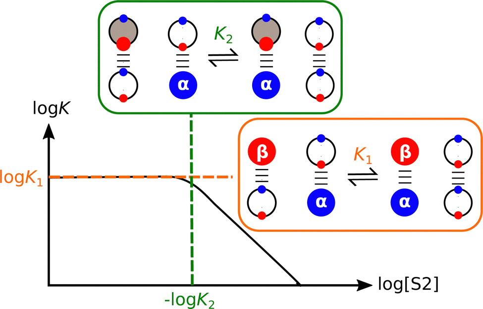 | ||
| Fig. 8 Relationship between the association constant (logK) for formation a complex between two solutes (α and β) and the composition of the solvent (log[S2]) for mixtures of a non-polar solvent (S1, white) and a polar aprotic solvent (S2, grey). The species that dominate at low concentrations of S2 are highlighted in the orange box. The green box highlights the competition between S1 and S2 for solvation of the H-bond donor (α), which leads to a decrease in log K at higher concentrations of S2. | ||
The association constant for formation of the 1:1 complex between 4-phenylazophenol and tri-n-butylphosphine oxide was measured in mixtures of n-octane as the non-polar solvent S1 and a number of different ethers and polyethers as the polar solvent S2.70 When the values of log K for all of alkane–ether mixtures were plotted as a function of the total concentration of ether oxygen atoms present in the solvent mixture ([O]), the same profile shown in Fig. 8 was obtained except with log[S2] replaced by log[O].70 This result shows that the solvation states of solutes are determined by the concentrations and the polarities of the functional groups present in a solvent. It makes no difference whether the oxygen acceptor sites in an ether solvent are all separated on different molecules or multiple oxygen acceptor sites are located on the same polyether molecule: the resulting solvation of H-bond donor solutes is indistinguishable. The implication for understanding solvation phenomena is that solvents can be described in a straightforward manner as a collection of independent non-covalent interaction sites (SSIPs). Competing solvation equilibria and interactions with solutes can be quantitatively predicted based on the concentrations and non-covalent interaction parameters of the SSIPs. This finding forms the basis for the Surface Site Interaction Model for the Properties of Liquids at Equilibrium (SSIMPLE), which is discussed in more detail below.
The solvent mixture experiment illustrated in Fig. 8 provided insight into the properties of alcohol solvents.71,72 When alcohols were used as the polar solvent (S2) in mixtures with n-octane (S1), the association constants measured for the formation of H-bonded complexes between two solutes showed a much more dramatic dependence on the concentration of S2 than had been observed for other polar solvents. The reason for the anomalous behaviour of alcohols is that they have both H-bond donor and H-bond acceptor sites, which leads to two important consequences.
The green box in Fig. 8 highlights how a polar aprotic solvent preferentially solvates H-bond donor solutes, reducing the observed association constant (logK). When alcohols are used as S2, the same preferential solvation of the H-bond donor solute occurs, but in this case, there is also preferential solvation of the H-bond acceptor solute, so at high concentrations of S2, the effect of an alcohol on log K is double that of a polar aprotic solvent, which only solvates one of the two solutes.71
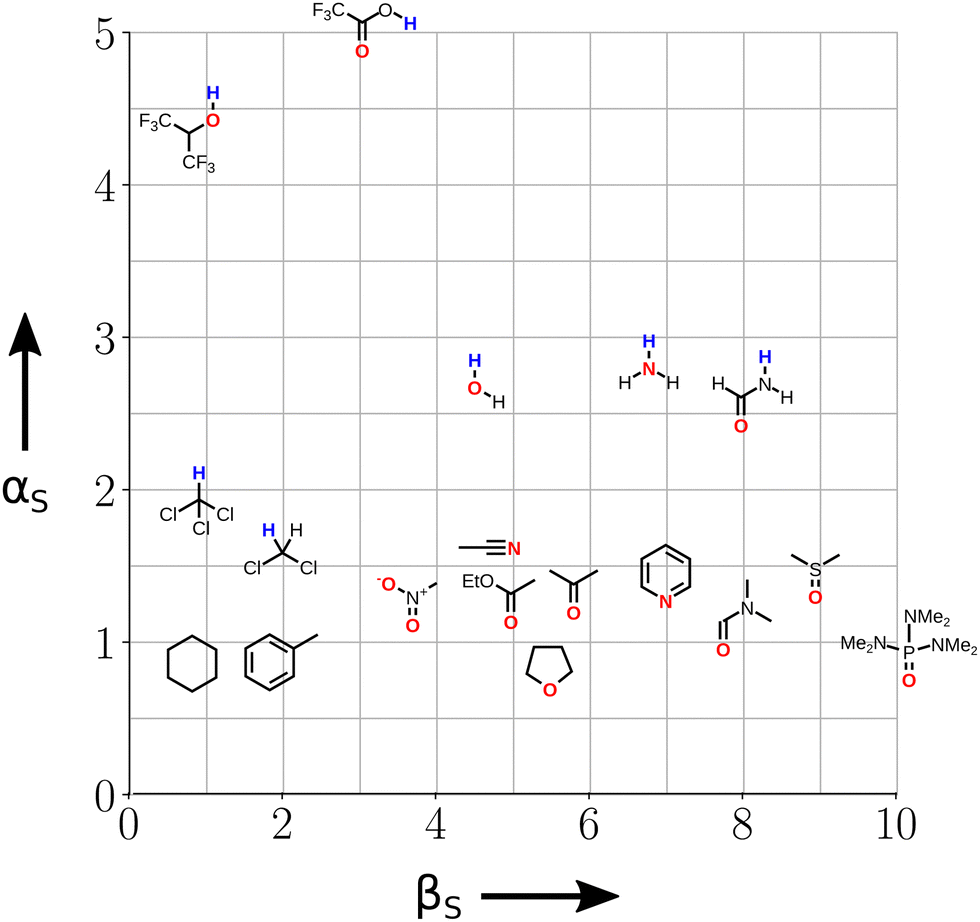
The other consequence of the presence of both H-bond donor and acceptor sites in alcohol solvents is that there is strong self-association. At high S2 concentrations, the H-bond donor and acceptor sites at the ends of the resulting oligomeric chains interact more strongly with solutes than the monomeric alcohols present at low S2 concentrations (Fig. 9). The solvent mixture experiments were used to determine αS and βS for alcohol solvents, and the values are significantly higher than the corresponding values of α and β measured for alcohols as monomeric solutes in dilute solution.72 The assumption that solute and solvent non-covalent interaction parameters can be used interchangeably breaks down for this class of solvents, but the behaviour appears to be unique to alcohols, and a large increase in polarity was not observed for secondary amides, which also self-associate into oligomeric chains.71
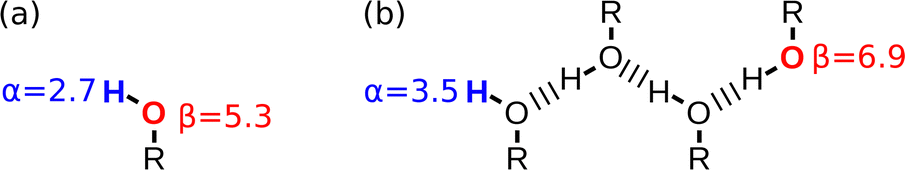 | ||
| Fig. 9 Non-covalent interactions parameters (α and β) measured for alcohols as (a) monomeric solutes in dilute solution and (b) solvents at high concentrations where oligomeric H-bonded chains predominate. | ||
2.3 Beyond the solution phase
Although the α and β parameters were derived using solution phase experiments, they can also be used to understand non-covalent interactions at surfaces and in the solid state. Fig. 10 depicts an Atomic Force Microscopy (AFM) experiment used to measure friction and adhesion properties due to non-covalent interactions between two macroscopic surfaces in the presence of a solvent. The tip of the AFM probe was functionalised with alcohols, the surface was functionalised with phosphonate diesters, and interactions were measured in solvent mixtures.74–76 The friction and adhesion between the tip and the surface were both large in alkanes, but when polar aprotic solvents were added, the strength of the surface interactions decreased. The relationship between the total energy of the surface contacts and solvent composition was exactly the same as that shown in Fig. 8 for solution phase solute–solute interactions. The concentration of polar solvent (S2) at which preferential solvation of the alcohol H-bond donor surface began to compete with the surface contacts was accurately predicted by using the relevant non-covalent interaction parameters in eqn (2) to estimate the equilibrium constant K2 for the solvation equilibrium shown in the green box in Fig. 8. | ||
| Fig. 10 An Atomic Force Microscopy (AFM) experiment to probe effect of solvent mixtures on surface adhesion and friction. The AFM tip was functionalised with H-bond donors (α), the surface was functionalised with H-bond acceptors (β), and measurements were made in a mixture of two different solvents (white and grey). | ||
The α and β parameters can also be used to accurately predict the relative probability of formation of different non-covalent interactions in the solid state.77,78 For example, for compounds that contain only one H-bond donor (α) and only two H-bond acceptors (β1 and β2), there are two possible modes of interaction in a crystal lattice (Forms I and II in Fig. 11). An analysis of crystal structures of such compounds using the Cambridge Structural Database (CSD)79 showed that the frequency of occurrence of Forms I and II can be accurately predicted based on the difference in interaction energy calculated using eqn (3).77
| ΔE/kJ mol−1 = −αβ1 + αβ2 | (3) |
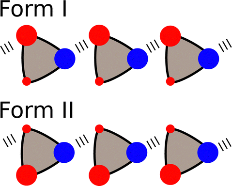 | ||
| Fig. 11 Compounds that contain one H-bond donor (blue) and two different H-bond acceptors (red) can adopt two different packing motifs in the solid state. | ||
Note that eqn (3) treats interactions in the solid using parameters derived from free energy measurements made in solution. The contributions of entropy to interactions in the solid and in solution are different, so ΔE is used to compare the relative probability of formation of different non-covalent interactions in a solid rather than to determine the free energy difference between two solids.
This idea can be generalised to an analysis of all pairwise functional group interactions in the CSD. The non-covalent interactions observed in a crystal structure are the outcome of a competition between different potential functional group interactions. The frequency of occurrence of an interaction between two specific functional groups in the CSD is therefore related to both the strength of this interaction and the strength of the alternative interactions that it had to compete with. A statistical analysis of the occurrence of non-covalent interactions in the CSD was used to make a quantitative ranking of the H-bond acceptor properties of different functional groups (RA). The solid state RA values obtained from the CSD correlate well with the corresponding β parameters measured in solution (Fig. 12).78 These analyses of interactions in solids, as well as at surfaces, indicate that the α and β parameters derived from solution phase experiments are not limited to liquids, but have general applicability for making quantitative predictions of non-covalent interaction energies in a range of different environments.
 | ||
| Fig. 12 Relationship between β parameters and solid state H-bond acceptor ratings RA for different functional groups. The best fit line is shown (R2 = 0.88).78 | ||
3 Ab initio calculation of non-covalent interaction parameters
The experimental α and β parameters quantify the relationship between chemical structure and the free energy change for the formation or exchange of non-covalent interactions, and describe the sum of all contributions to the interaction energy, i.e. changes in electrostatics, polarisation, dispersion and entropy. One approach to the development of a computational method for obtaining the non-covalent interaction parameters would be to evaluate each of these contributions using a sufficiently high level of theory.80 An alternative is to correlate the empirical α and β parameters with computed molecular descriptors that can be obtained in a straightforward manner using density functional theory (DFT),81–87 and this is the approach we have opted for.11 The most striking correlation was found with the maximum (Emax) and minimum (Emin) of the Molecular Electrostatic Potential (MEP) calculated at the 0.002 e bohr−3 isodensity surface, which approximates the van der Waals surface.88Fig. 13 shows that the experimentally determined values of α and β can be accurately reproduced by eqn (4) and (5) using the calculated MEP values.| α = 1.2 × 10−5Emax2 + 1.14 × 10⁻²Emax | (4) |
| β = cFG(8.33 × 10⁻⁵Emin2 − 2.08 × 10⁻²Emin) | (5) |
 | ||
| Fig. 13 Comparison of non-covalent interaction parameters calculated using eqn (4) and (5) with the corresponding experimental values. (a) α (RMSE = 0.32) (b) β (RMSE = 0.64).11 | ||
This result suggests that the exchange of solute and solvent interactions illustrated in Fig. 2 is dominated by differences in electrostatic interactions and that the other contributions largely cancel out. However, the relationships in eqn (4) and (5) are both quadratic, and additional functional group specific constants (cFG) were required to obtain accurate values of the β parameter, which implies that other factors also play a role.
4 Surface site interaction points
The availability of a computational method for obtaining non-covalent interaction parameters allowed the development of a general treatment of intermolecular interactions, which we call the SSIP approach. Experimental non-covalent interaction parameters can only be determined for the most polar site on the surface of a molecule, but Fig. 13 shows that these experimentally determined values of α and β correlate well with the calculated MEP values for the most polar site on the van der Waals surface. Since the MEP can be calculated across the entire surface of the molecule, it is possible to describe all possible interactions at all points on the molecular surface in the same way. Whereas the experimental approach described previously only focuses on the most polar site of interaction, with a computational approach we can get a more complete picture of how a molecule interacts with the environment.The number of simultaneous interactions that a molecule can make is limited by steric packing of the interacting partners, so a molecular surface is described as a finite number of SSIPs. The area of an SSIP is defined based on the footprint of a H-bonding interaction at the van der Waals surface (9 Å2).10 A footprinting algorithm was developed to convert the MEP surface of a molecule into a set of SSIPs, where each SSIP is described by a non-covalent interaction parameter (α or β) calculated using eqn (4) and (5) and the value of Emax or Emin for the patch of surface under that footprint.11,89Fig. 1 illustrates the results for methanol and pyridine, showing how the SSIP description captures the properties of both polar and non-polar interaction sites. The COSMO methodology developed by Klamt et al. also uses surface patches to characterise non-covalent interactions across the entire surface of a molecule.90,91 However, an important difference between the COSMO and SSIP methods is the use of empirical calibration. SSIPs represent surface patches that correspond to the area involved in a H-bonding interaction, which means that the SSIP non-covalent interaction parameters can be calibrated by using experimental data on H-bonded complexes to make a direct connection between ab initio MEP calculations and solution phase free energies (Fig. 13).
Experimental data on vapour–liquid equilibria for noble gases and alkanes show that van der Waals or dispersion interactions are proportional to molecular surface area, regardless of atom type.92 The use of SSIPs that each represent the same area on the van der Waals surface therefore provides a relatively straightforward treatment of dispersion, because the contribution to SSIP interactions can be treated as a constant (EvdW = −5.6 kJ mol−1).92 For solution phase equilibria such as the solvent competition model shown in Fig. 2, contributions due to the exchange of dispersion interactions largely cancel out, because there is an exchange of surface contacts of equal surface area: there are two SSIP interactions on each side of the equilibrium.18,93 However, the magnitude of the dispersion contribution becomes important for an accurate description of phenomena where the number of SSIP contacts changes, for example in the hydrophobic effect (see below).92 There is also experimental evidence that the contribution from van der Waals interactions does not fully cancel out in solution phase interactions between aromatic rings, where there is exceptionally good geometric complementarity,94 and in the interactions between perfluorocarbons, which pack poorly.92,95
4.1 SSIP interactions in the solid state
Etters analysis of non-covalent interactions in crystal structures suggests that packing is dictated to a first approximation by hierarchical formation of the most polar interactions.96 This idea can be used to predict the pairing of SSIPs in crystal structures, and hence estimate the relative stabilities of different solids. Fig. 14 illustrates how SSIPs are likely to be paired in a cocrystal of two different compounds. The overall energy is minimised if the SSIP with the largest α interacts with the SSIP with the largest β, the second best α interacts with the second best β and so forth. The total SSIP pairing energy of the crystalline solid (E) is obtained by summing over all contacts (eqn (6)).97,98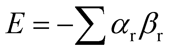 | (6) |
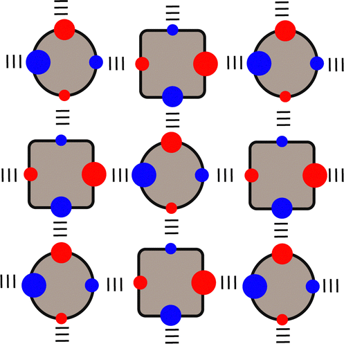 | ||
| Fig. 14 SSIP interactions in a cocrystal of two different compounds. Packing is dictated by hierarchical organisation of SSIP contacts based on polarity, which is indicated by the size of the circles representing the SSIPs: large α pairs with large β and small α pairs with small β. | ||
An alternative packing arrangement for these compounds would be crystallisation separately as the pure substances. Eqn (6) can be used to calculate the difference between the SSIP pairing energy for the cocrystal and SSIP pairing energies for the two pure substances. This calculated energy difference has been successfully used as a selection tool in virtual screening of large compound libraries to identify coformers that have a high probability of forming cocrystals with an active pharmaceutical ingredient (API).99,100 For example, new cocrystals of nalidixic acid, sildenafil, griseofulvin and spironolactone have been discovered using the SSIP virtual screening method.98,101,102
4.2 SSIP interactions in solution
A number of approaches have been developed to compute solvation energies based on empirical H-bond parameters103–107 and on an analysis of the MEP.90,91,108,109 Solvation free energies can also be obtained by considering pairwise interactions between SSIPs.Treatment of SSIP interactions in the solid state is relatively straightforward, because the molecules are static and closely packed, so that each SSIP is in contact with a partner. In solution, all possible SSIP interactions are in dynamic equilibrium, and there are void spaces, so that non-bound states are also accessible. Fig. 15 illustrates non-covalent interactions in a solution phase mixture of a solute (square) and solvent (circles). The dots represent the relatively large volume of void space present in a liquid (approximately 45% for organic solvents at room temperature).10 The probability of forming an interaction between two SSIPs, i and j, is given by the equilibrium constant Kij in eqn (7).10
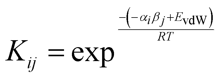 | (7) |
 | ||
| Fig. 15 SSIP description of a solution of a solute (square) dissolved in a solvent (circle). There are multiple competing equilibria between SSIP contacts, and there are void spaces (dots), so that not all SSIPs are paired. | ||
The inclusion of the van der Waals term in the interaction energy (EvdW) is important for accurately describing the probability of formation of non-bonded states, which do not make van der Waals interactions and are treated as contact with void space.
The solution phase can therefore be treated as a Boltzmann ensemble of all possible SSIP interactions, and the matrix of Kij values calculated using eqn (7) can be used to determine the speciation of intermolecular contacts for any mixture of solvents and solutes. The Surface Site Interaction Model for the Properties of Liquids at Equilibrium (SSIMPLE) is a general implementation of this approach that is used to calculate solvation free energies from the SSIP description of molecules. The method is described in detail elsewhere,10,11,110 but the assumption is that SSIPs can adopt either bonded or non-bonded states, and that the non-bonded state has the same potential energy in any environment. For an individual SSIP in a given phase, calculation of the speciation of intermolecular contacts is used to obtain the total amount that interacts with other SSIPs and how much is non-bonded. These concentrations give an effective equilibrium constant for interaction of a single SSIP with the solvent environment and are used to calculate the solvation free energy of the SSIP relative to an infinitely dilute phase, where there are no intermolecular interactions.
Fig. 16 shows how the solvation free energy (ΔGS) calculated for a single SSIP varies with non-covalent interaction parameter in different solvent environments. n-Hexadecane (grey) is a non-polar solvent, so the interaction is dominated by the van der Waals term, and the solvation free energy does not depend strongly on the polarity of the SSIP. Chloroform (blue) has a relatively polar CH group, which strongly solvates negative SSIPs with large β parameters. However, there are no polar negative sites in chloroform, so the solvation profile is similar to n-hexadecane for positive SSIPs. THF (red) has a polar H-bond acceptor but no polar positive sites, so it solvates positive SSIPs with large α parameters strongly but behaves similarly to n-hexadecane for negative SSIPs. Water (black) has both H-bond donor and acceptor sites, so it solvates SSIPs with either large α or large β values strongly. However, water is unique in that the solvation free energy is positive for non-polar solutes. The solvation profile in Fig. 16 shows that for SSIPs with values between −1.5 and +1.0, the water–water interaction is more favourable than the water–solute interaction. This behaviour is a manifestation of the hydrophobic effect and shows that this phenomenon can be understood simply based on competition for pairwise interactions between solvent and solute. Solvation profiles such as those illustrated in Fig. 16 can be used in a quantitative manner to calculate solvent similarity indices to compare the solvation properties of different solvents with respect to all possible solutes. Solvent similarity indices provide a tool for the design of cost effective or environmentally-friendly alternatives to conventional solvents.111
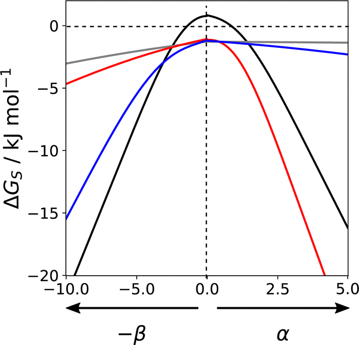 | ||
| Fig. 16 Solvation free energies (ΔGS) calculated for a single SSIP as a function of non-covalent interaction parameter (α or β) in different solvents: n-hexadecane (grey), chloroform (blue), THF (red), water (black) at 298 K. | ||
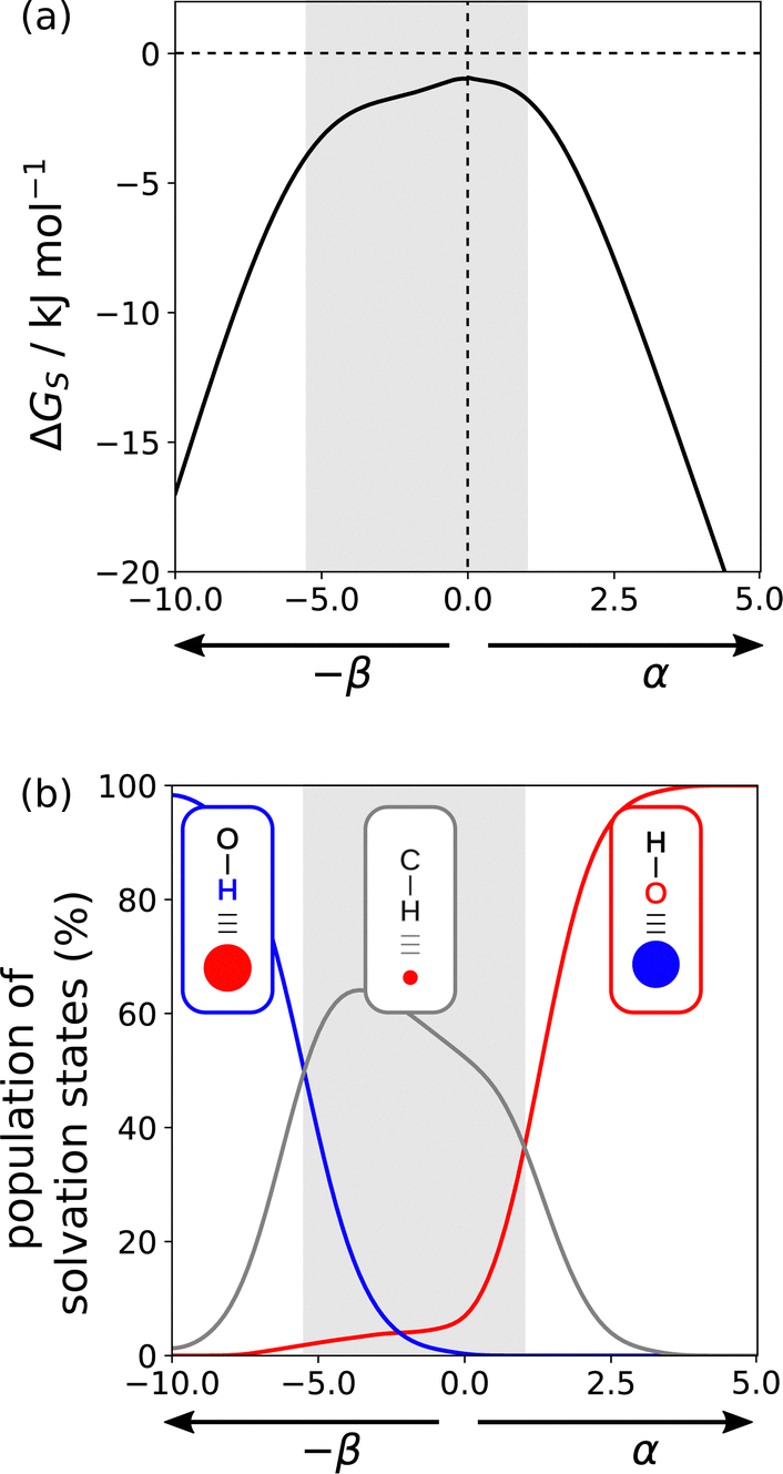
Fig. 17(a) shows the solvation profile for ethanol, which is a more complex solvent than the examples shown in Fig. 16, because it contains both polar and non-polar functional groups. Three different solvation regimes are apparent, and the changes in gradient in 17a are indicative of changes in the polarity of the solvent functional group that interacts with the solute. Fig. 17(b) shows the populations of the three different solvation states that determine the properties of ethanol. Negative SSIPs with large β values are solvated by the OH H-bond donor of ethanol (blue line). Negative SSIPs with β values less than 6.9 are solvated by the CH groups of ethanol (grey line). The reason for this switch from solvation by OH to CH is that the β value of the H-bond acceptor sites associated with the oxygen lone pairs of ethanol is 6.9. The concentration of solvent is overwhelmingly higher than the concentration of the solute, so solutes with negative SSIPs that are less polar than the solvent will be outcompeted for interaction with solvent OH H-bond donors. In the third regime in 17a, positive SSIPs are preferentially solvated by the H-bond acceptor sites associated with the oxygen lone pairs of ethanol (red line in 17b). The red and blue lines in 17b show that the total population of solvation states is nearly 100% for polar SSIPs with large α or β values. For non-polar SSIPs, solvation is dominated by the van der Waals term, so the grey line in 17b only reaches a maximum of 60% and there is 40% of the non-bonded state.
 | ||
| Fig. 17 (a) Solvation free energies (ΔGS) calculated for a single SSIP as a function of non-covalent interaction parameter (α or β) in ethanol. The shading highlights three different solvation regimes. (b) Population of solvation states of a single SSIP in ethanol plotted as a function of non-covalent interaction parameter (α or β). The blue line shows solvation by the OH H-bond donor, the red line solvation by the oxygen H-bond acceptor and the grey line solvation by the CH groups. | ||
Solvation profiles can also be used to obtain insights into the properties of solvent mixtures. Fig. 18(a) compares the solvation profiles of chloroform (blue), THF (red) and a 1:1 mixture (black). The solvation profile of the mixture closely resembles THF for positive SSIPs, whereas for negative SSIPs, the solvation profile of the mixture is closer to chloroform (blue). Fig. 18(b) provides an explanation for this behaviour. The blue line shows the extent to which SSIPs are solvated by chloroform in the mixed solvent, and the red line shows the proportion of SSIPs solvated by THF. The CH group in chloroform is more polar than the CH groups in THF, so chloroform preferentially solvates negative SSIPs. The H-bond acceptors sites associated with the oxygen lone pairs of THF are more polar than any of the negative sites in chloroform, so THF preferentially solvate positive SSIPs. For non-polar SSIPs, the van der Waals term dominates, so there is an equal probability of interaction with either of the two solvents. One consequence of the preferential solvation illustrated in Fig. 18 is that interactions between two polar solutes are generally less favourable in mixtures than in the pure solvents because they are more strongly solvated.
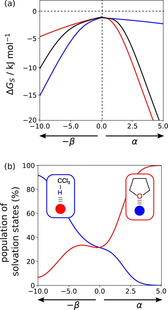 | ||
| Fig. 18 (a) Solvation free energies (ΔGS) calculated using SSIMPLE for a single SSIP as a function of non-covalent interaction parameter (α or β) in chloroform (blue), THF (red), and a 1:1 mixture of chloroform and THF (black). (b) Population of solvation states of a single SSIP in a 1:1 mixture of chloroform and THF plotted as a function of non-covalent interaction parameter (α or β). The blue line shows solvation by chloroform, and the red line shows solvation by THF. | ||
:1 complex between two solutes. Thus the difference between the free energy change for formation of an interaction between two solute SSIPs (−αβ + EvdW) and the sum of the two solute SSIP solvation free energies can be used to make predictions about solvent effects on association constants for formation of intermolecular complexes.110Fig. 19 compares calculated and experimental values for 351 different complexes in 12 different solvents (RMSE in logK = 0.37), and the values calculated using SSIMPLE solvation free energies have comparable accuracy to association constants predicted using empirical solvent parameters in eqn (3) (RMSE in logK = 0.29).20,112,113
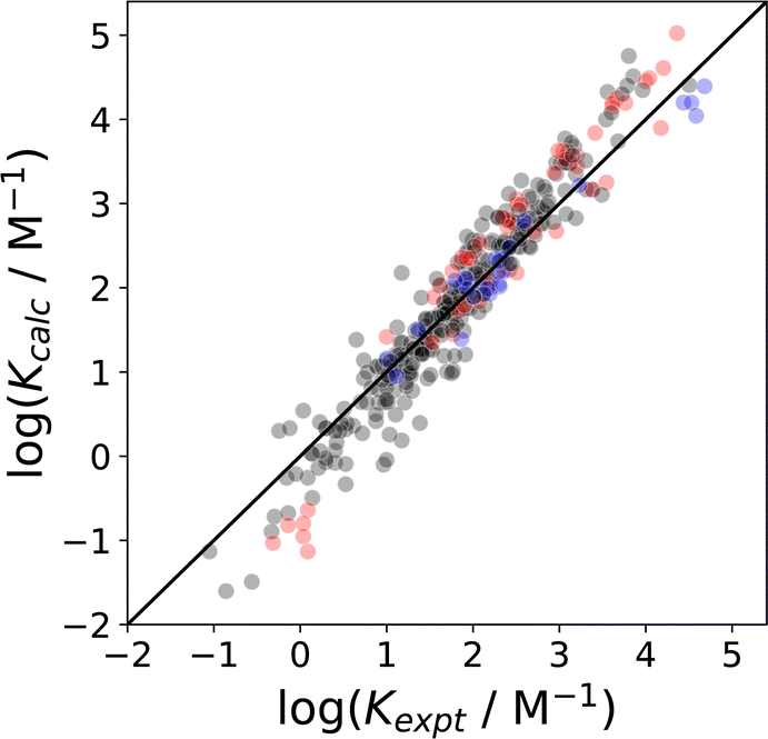 | ||
| Fig. 19 Comparison of association constants (logK) for formation of 1:1 complexes between two solutes calculated using SSIMPLE with the corresponding experimental values (RMSE in logK = 0.37) for 351 complexes involving a range of different solutes and solvents (1,1,1-trichloroethane, 1,2-dichloroethane, benzene, chlorobenzene, chloroform, cyclohexane, dichloromethane, n-heptane, n-hexane, o-dichlorobenzene, acetonitrile, acetone).20,112,113 The black points are interactions between neutral compounds, red points indicate that one of the compounds is an anion, and blue points indicate that one of the compounds is a cation. The line corresponds to y = x. | ||
The advantage of the SSIMPLE approach over the use of empirical parameters in eqn (2) is that SSIMPLE can be applied to any solvent mixture of any composition and predictions can be made for solvents for which experimental parameterisation is not possible. Fig. 20 shows that SSIMPLE provides an excellent description of the effect of solvent composition on the association constant for formation of a 1:1 complex between tri-n-butylphosphine oxide 4-phenylazophenol.69,71 This complex was studied in mixtures of n-octane (S1) and seven more polar solvents (S2). For each solvent mixture, the relationship between log K and log[S2] follows the general trend illustrated in Fig. 7, and SSIMPLE accurately predicts the concentration of S2 at which preferential solvation starts to compete with the solute–solute interaction in each case.
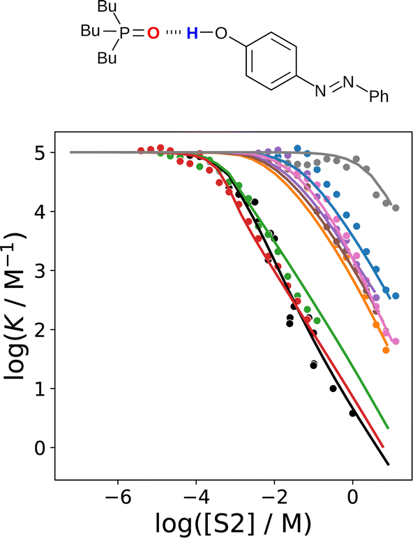 | ||
| Fig. 20 The association constant (logK) for formation a 1:1 complex between tri-n-butylphosphine oxide and 4-phenylazophenol in mixtures of n-octane (S1) and a more polar solvent (S2) plotted as a function of solvent composition (log[S2]). S2 is di-n-butyl sulfoxide (red), N,N-diethyl acetamide (green), 2-ethylhexyl-acetamide (black) 2-heptanone (orange), ethyl heptanoate (brown), di-n-octyl ether (purple), n-butyl cyanide (pink), 1,1,2,2-tetrachloroethane (blue) and toluene (grey). The points are experimental measurements,69,71 and the lines were calculated using SSIMPLE. | ||
SSIMPLE can also be used to construct quantitative versions of the generic Functional Group Interaction Profile (FGIP) shown in Fig. 4 for any solvent or solvent mixture, providing a useful design tool for guiding the choice of functional group or solvent composition in order to optimise the relative contributions of different types of non-covalent interaction.110Fig. 21 shows the SSIMPLE FGIP for water. There are two regions in which functional group interactions are favourable and two regions where interactions with the solvent dominate (cf. Fig. 4). The value of ΔΔG for the interaction between two non-polar solutes in the solvophobic quadrant is about −3 kJ mol−1. This result differs from the prediction obtained using eqn (1), which gives a value of ΔΔG of about −12 kJ mol−1. The reason for the difference is that the solvent competition model illustrated in Fig. 2 assumes that interactions with the solvent are either fully made or fully broken. In water, the solvent shell around non-polar solutes reorganises to minimise the disruption of water–water H-bonds, and consequently there is less H-bonding to be gained on desolvation. In other words, the gain in solvent–solvent interactions on the right hand side of the equilibrium in Fig. 2 is only a quarter of a H-bond rather than a full water–water interaction, because both solvents on the left hand side of the equilibrium retain 75% of a H-bond with the surrounding solvent. These solvation equilibria are accurately described by the SSIMPLE treatment, and the resulting value of ΔΔG is consistent with experimental data on the magnitude of the hydrophobic effect. For example, the contribution of the hydrophobic effect to the stability of biomolecular complexes is 0.3 kJ mol−1 per Å2 of buried non-polar surface, which corresponds to −3 kJ mol−1 for the interaction between two non-polar SSIPs with a contact surface area of 9 Å2.114
 | ||
| Fig. 21 FGIP for water calculated using SSIMPLE. Red regions represent unfavourable interactions, blue regions represent favourable interactions, and the contours are labelled with ΔΔG values in kJ mol−1. Representative solute functional groups are illustrated (reproduced from ref. 110 with permission from RSC Publishing, copyright 2020). | ||
Fig. 22 shows how the FGIP of water changes when cosolvents are added. In a mixture of water and THF, the hydrophobic region disappears, but the other three quadrants are unaffected (Fig. 22(a)). The reason for this behaviour is that in a mixture of water and THF non-polar solutes are preferentially solvated by the CH groups of THF. As a result, the driving force for the hydrophobic effect is eliminated, because no water–water H-bonds are formed when the solutes are desolvated. In a mixture of water and HMPA, the hydrophobic quadrant again disappears due to preferential solvation of non-polar solutes by the CH groups of the cosolvent (Fig. 22(b)). In this case, the favourable interactions between polar solutes in the other blue quadrant of the FGIP are also suppressed. The reason for this behaviour is that HMPA has an exceptionally polar H-bond acceptor (β = 10.9), so H-bond donor solutes are more strongly solvated in the mixed solvent than in pure water. Quantitative measurements of the effects of cosolvents on protein denaturation show that THF and HMPA are two of the most effective solvents at unfolding proteins, and the FGIPs in Fig. 22 provide an explanation.115
 | ||
| Fig. 22 (a) FGIP for an equimolar mixture of water and THF. (b) FGIP for an equimolar mixture of water and HMPA. Red regions represent unfavourable interactions, blue regions represent favourable interactions, and the contours are labelled with ΔΔG values in kJ mol−1 calculated using SSIMPLE.110 | ||
The generalised FGIP in Fig. 4 suggests that all polar protic solvents should show solvophobic properties similar to water, but this is not necessarily the case. Fig. 23 shows the FGIPs for two polar protic solvents where the solvophobic quadrant is absent. The FGIP for ethanol (Fig. 23(a)) resembles the FGIP for a mixture of water and THF shown in Fig. 22(a), and the reasons for the absence of a solvophobic region are similar. In ethanol, non-polar solutes are solvated by the non-polar CH groups of ethanol rather than the polar OH group (see Fig. 17(b)), and so the new solvent–solvent interactions that are made when non-polar solutes are desolvated are not H-bonds. Exchange of non-polar contacts leads to no overall change in interaction energy, so the bottom left quadrant of the FGIP is now white rather than blue. Fig. 23(b) shows the FGIP for liquid ammonia. In this case, the solvent has one H-bond acceptor and three H-bonds donors, so oligomeric chains of H-bonded solvent molecules predominate. However, only one of the three H-bond donors can be paired, and the excess H-bond donors present in the solvent are always available for interaction with H-bond acceptor solutes.116 The result is that the corresponding red quadrant where solute–solvent interactions dominate is enlarged to fill most of the bottom half of the FGIP, and the solvophobic quadrant disappears. Solvophobic effects are only observed if the solvation of a non-polar solute has to compete with polar solvent–solvent interactions. If the solvent has additional interaction sites that are not fully H-bonded, these sites will be used to solvate non-polar solutes, and there is no solvophobic region in the FGIP. Other than water, two solvents that have an FGIP with a large solvophobic quadrant are formamide and ethylene glycol, which is consistent with Abrahams experimentally determined solvophobicity scale.103,110
 | ||
| Fig. 23 (a) FGIP for ethanol (b) FGIP for ammonia. Red regions represent unfavourable interactions, blue regions represent favourable interactions, and the contours are labelled with ΔΔG values in kJ mol−1 calculated using SSIMPLE.110 | ||
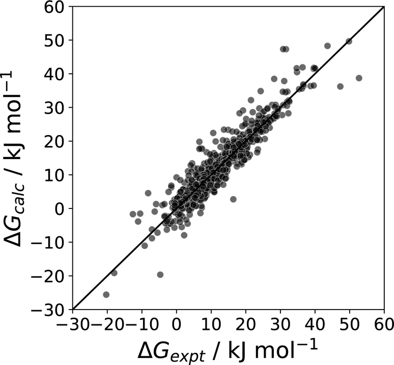 | ||
| Fig. 24 Comparison of calculated and experimental phase transfer free energies (ΔG, mole fraction standard state) for transfer of 214 compounds from n-octanol to water n-hexadecane to water, 177 compounds from the pure liquid to water, 177 compounds from the pure liquid to n-hexadecane, and for transfer of water from water to 115 different pure liquids (RMSE = 3.4 kJ mol−1).11 | ||
Phase transfer free energies calculated using SSIMPLE have been used to parametrise beads that are used to represent fragments of molecules in Dissipative Particle Dynamics (DPD) simulations. The SSIMPLE approach is ideally suited to the description of molecular fragments, since any SSIPs that would sit at the junction point between two fragments in the complete molecule can be removed and do not contribute to the calculated solvation energies. A DPD description of a range of surfactants has been developed using this methodology, and simulations of aqueous solutions of these compounds accurately predict self-assembly properties such as critical micelle concentration and aggregation number.117,118
5 Limitations
The examples above highlight areas in which SSIPs and SSIMPLE can be used to make useful quantitative predictions about the free energy changes associated with formation or exchange of non-covalent interactions. However, there are some limitations to the current methodology.5.1 Temperature
Eqn (4) and (5) that are used to convert the ab initio MEP surface into the non-covalent interaction parameters, α and β, are based on experimental measurements that were carried out at 298 K. Although it should be possible to generalise the treatment to different temperatures, additional methodology is required.1195.2 Ionic interactions
Although α and β parameters for ions have been measured, the experiments are restricted to interactions with a neutral binding partner. For two charged species, long-range Coulombic interactions are likely to play an important role, so non-covalent interactions between charged solutes and the solvation properties of ionic liquids are beyond the scope of the current treatment.120 In addition, it is not possible to use DFT to calculate SSIPs for an ion, because the MEP calculated in the gas phase is dominated by the Coulombic interaction with the overall molecular charge.5.3 Conformational equilibria
The treatment described above uses a single conformation of a molecule to calculate SSIPs. For flexible molecules, the choice of conformation can affect the functional groups that are exposed on the van der Waals surface. As a consequence, the SSIP description of a molecule can change with conformation and is not defined by the atomic connectivity. One advantage is that changes in the polarity and number of SSIPs reflects differences in the non-covalent interaction properties of different conformations, but a disadvantage is that treatment of flexible molecules requires calculation of an SSIP description for each conformer. Consider a molecule that can adopt two conformations, one of which is folded to make an intramolecular H-bond and one which is extended with no intramolecular interactions. In the extended conformer, all of the SSIPs describing all of the functional groups will manifest on the van der Waals surface. In the folded conformer, the two SSIPs involved in the intramolecular interaction will be buried, and footprinting of the van der Waals surface will generate two fewer SSIPs than the extended conformer. The population of these two conformers will depend on the solvent environment, so consideration of conformational ensembles is required for an accurate description of these systems.10,121 The development of a fully predictive approach requires a method for combining the free energy contributions due to non-covalent interactions calculated using SSIPs with conformational energy differences calculated using a different computational method, such as DFT.122 Studies on molecular balances have begun to tackle this problem. The equilibrium between two well-defined conformations can be used to quantify solvent effects on an intramolecular non-covalent interaction that is formed in one conformer and not in the other. This molecular balance experiment is equivalent to the equilibrium shown in Fig. 2, except that the two functional groups are part of the same molecule. The sensitivity of these systems to small free energy differences allows very weak interactions to be investigated. The results have been rationalised using eqn (1) and can be used to investigate the balance between covalent torsional energies and non-covalent interaction energies.62,1235.4 Allosteric cooperativity
The SSIMPLE approach assumes that all SSIPs are independent of one another, so that an interaction made with one SSIP does not have any effect on the properties of the other SSIPs in the molecule. There is experimental evidence that this assumption does not hold in some situations, and significant allosteric cooperativity has been observed between two different interaction sites on the same functional group. For example, formation of a H-bond with one of the lone pair sites on a carbonyl oxygen causes a significant decrease in the β parameter for interaction at the second lone pair site.124,125 Conversely, formation of an H-bond with an alcohol or amide oxygen leads to a significant increase in the α parameter of the OH hydrogen and the NH hydrogen respectively (see Fig. 9).72,126–128 Polarisation has also been shown to affect aromatic interactions.129 The magnitude of these allosteric effects is likely to depend on the nature of interacting partners, so a treatment that goes beyond pairwise interactions is required to describe this phenomenon.5.5 Chelate cooperativity
The treatment of intermolecular complexes described above deals with single point interactions between two functional groups. However, most complexation processes involve multiple intermolecular contacts at many sites on the surfaces of the two molecules. In addition to simply summing the free energy contributions from each intermolecular interaction, the chelate cooperativity associated with formation of multiple interactions must be considered.56 Effective molarity (EM) is used to experimentally quantify chelate cooperativity, and a wide range of different values have been reported for different supramolecular systems (10−3 to 103 M).130–132 However, there are no reliable theoretical methods for predicting the value of EM. Chelate cooperativity will also play a role in describing the properties of solvents which have adjacent H-bond donor and H-bond acceptor sites. For example, in carboxylic acids, the solvent–solvent interaction involves cooperative formation of two intermolecular H-bonds.71,133 Similarly, carboxylic acid solvents can make cooperative interactions with solutes that have adjacent H-bond donor and H-bond acceptor sites. The treatment of such systems depends on the geometrical complementarity of the two interacting molecular surfaces and is beyond the scope of the current SSIMPLE approach, where all SSIPs are considered to act independently.5.6 Three-dimensional structure
Although the SSIP description of a molecule defines a location in space for each SSIP, this information is not used in any of the examples discussed here. The SSIPs are simply used to determine the free energy contributions from pairwise interactions, and each interaction site is treated independently. The advantage of this approach is that calculations are fast, because it is not necessary to compute three-dimensional structures or interaction geometries. The underlying assumption is that when two SSIPs interact, the arrangement of the two interacting groups is sufficiently close to ideal that the interaction energy can be considered a constant given by (−αβ + EvdW). This assumption is reasonable for systems where any two molecules make a single SSIP contact, because the molecules are free to adopt the optimal geometry. However for systems where there are significant geometric constraints, it may not be possible for all intermolecular contacts to attain a suitable geometrical arrangement, and then the SSIP interaction energies will be less favourable. For example, interactions between molecules in confined spaces and solvation of small cavities can show quite different behaviour from solution phase processes, and the treatment of such systems would require some consideration of the distance and angular dependence of the SSIP interaction energies.134,1355.7 Covalent bonding
For specific combinations of functional groups, covalent interactions can be significant. These complexes show quite different behaviour from the non-covalent systems discussed in this review.136 A good example is the 1:1 complex formed between molecular iodine and tetramethyl thiourea, which has been studied in 15 different solvents. Solvent effects on the stability of this complex are quite different from closely related halogen-bonded and H-bonded complexes (Fig. 25). Using the non-covalent interaction parameter α for molecular iodine in eqn (2) accurately predicts the association constants measured for the halogen-bonded complex formed with tetramethyl urea (green points). Similarly, the β values for both tetramethyl urea and tetramethyl thiourea and accurately predict the association constants measured for the H-bonded complex formed with 4-azophenylphenol (blue and red points respectively). In contrast, the iodine–tetramethyl thiourea complex is four orders of magnitude more stable than predicted by eqn (2) (black points). Spectroscopic and structural evidence supports the conclusion that a significant covalent contribution leads to the anomalous stability. A survey of cocrystals of molecular iodine and thiocarbonyl compounds in the CSD shows that short intermolecular sulfur–iodine distances are correlated with increases of up to 0.4 Å in the iodine–iodine bond length.57
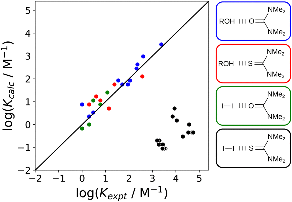 | ||
| Fig. 25 Comparison of association constants (logK) for formation of 1:1 complexes calculated using eqn (2) with the corresponding experimental values for four different complexes in 15 different solvents.57 The structures of the complexes are shown, and the colouring of the boxes indicates which data points belong to which complex. The line corresponds to y = x. | ||
Covalent interactions probably make a contribution in all of the complexes discussed in this review, but in most cases, these effects are small enough to be captured as perturbations in the empirical values of the non-covalent interaction parameters α and β. Observation that a complex is significantly more stable than predicted by the non-covalent interaction parameters is an indication that covalent contributions may be important.57,137,138
6 Conclusion
This review summarises twenty years of research on a surface-based approach to describing non-covalent interactions. Molecules are described by a discrete set of points on the van der Waals surface, SSIPs, which represent all possible interactions that can be made with another molecule. The definition of an SSIP is based on the thermodynamic properties of H-bonding interactions measured in solution and the geometrical properties of H-bonding interactions observed in the solid state. However, the approach is more generally applicable to all classes of non-covalent interaction, including halogen-bonds, aromatic interactions and interactions between non-polar functional groups. Ab initio calculations can be used to obtain the non-covalent interaction parameters, α and β, that describe the properties of SSIPs, and the strength of the interaction between two SSIPs is related to the product of the two interaction parameters, −(α × β). The contribution due to non-polar or dispersion interactions is treated as a constant, because all SSIPs represent the same contact area on the van der Waals surface. A molecular ensemble, such as a solution containing multiple solutes and solvents, is simply treated as a collection of SSIPs, and the speciation of all pairwise SSIP interactions is used to calculate thermodynamic properties such as solvation free energies and equilibrium constants. This approach has been implemented in the SSIMPLE algorithm, which provides reliable predictions of partition coefficients and solvent effects on the association constants for formation of intermolecular complexes (calculated free energies are generally accurate to within a few kJ mol−1). A virtual screening tool that uses SSIPs to predict the probability of cocrystal formation has successfully identified multiple new API cocrystals. Nevertheless, there are some limitations to the SSIP approach, and future directions that would improve the generality of the methods have been outlined.Software that can used to footprint a molecule in order to obtain the SSIP description and to calculate solvation energies using SSIMPLE is freely available at https://gitlab.developers.cam.ac.uk/ch/hunter/ssiptools. More details can be found in ref. 89.
Conflicts of interest
There are no conflicts to declare.Acknowledgements
We thank S. Thompson and Dr M. D. Driver for collating the α and β dataset. We thank Dr D. P. Reynolds, Dr M. C. Misuraca, J. Baixeras Buye, B. Csakany, A. Lorusso Notaro Francesco and D. Soloviev for their feedback.Notes and references
- J. Černý and P. Hobza, Phys. Chem. Chem. Phys., 2007, 9, 5291–5303 RSC.
- K. Müller-Dethlefs and P. Hobza, Chem. Rev., 2000, 100, 143–168 CrossRef PubMed.
- L. Jean-Marie, From Supermolecules to Supramolecular Assemblies, John Wiley & Sons, Ltd, 1995, ch. 7, pp. 81–87 Search PubMed.
- M. Raynal, P. Ballester, A. Vidal-Ferran and P. W. N. M. van Leeuwen, Chem. Soc. Rev., 2014, 43, 1660–1733 RSC.
- M. Raynal, P. Ballester, A. Vidal-Ferran and P. W. N. M. van Leeuwen, Chem. Soc. Rev., 2014, 43, 1734–1787 RSC.
- M. H. Abraham, Chem. Soc. Rev., 1993, 22, 73–83 RSC.
- M. J. Kamlet, J. L. M. Abboud, M. H. Abraham and R. W. Taft, J. Org. Chem., 1983, 48, 2877–2887 CrossRef CAS.
- D. Qiu, P. S. Shenkin, F. P. Hollinger and W. C. Still, J. Phys. Chem. A, 1997, 101, 3005–3014 CrossRef CAS.
- E. M. Duffy and W. L. Jorgensen, J. Am. Chem. Soc., 2000, 122, 2878–2888 CrossRef CAS.
- C. A. Hunter, Chem. Sci., 2013, 4, 1687–1700 RSC.
- C. S. Calero, J. Farwer, E. J. Gardiner, C. A. Hunter, M. Mackey, S. Scuderi, S. Thompson and J. G. Vinter, Phys. Chem. Chem. Phys., 2013, 15, 18262–18273 RSC.
- R. W. Taft and M. J. Kamlet, J. Am. Chem. Soc., 1976, 98, 2886–2894 CrossRef CAS.
- M. J. Kamlet and R. W. Taft, J. Am. Chem. Soc., 1976, 98, 377–383 CrossRef CAS.
- C. Reichardt and T. Welton, Solvents and solvent effects in organic chemistry, John Wiley & Sons, 2010 Search PubMed.
- M. H. Abraham, H. S. Chadha, G. S. Whiting and R. C. Mitchell, J. Pharm. Sci., 1994, 83, 1085–1100 CrossRef CAS PubMed.
- D. Gurka and R. W. Taft, J. Am. Chem. Soc., 1969, 91, 4794–4801 CrossRef CAS.
- E. M. Arnett, L. Joris, E. Mitchell, T. S. S. R. Murty, T. M. Gorrie and P. v R. Schleyer, J. Am. Chem. Soc., 1970, 92, 2365–2377 CrossRef CAS.
- C. A. Hunter, Angew. Chem., Int. Ed., 2004, 43, 5310–5324 CrossRef CAS PubMed.
- J. Cook, C. Hunter, C. Low, A. Perez-Velasco and J. Vinter, Angew. Chem., Int. Ed., 2007, 46, 3706–3709 CrossRef CAS PubMed.
- R. Cabot, C. A. Hunter and L. M. Varley, Org. Biomol. Chem., 2010, 8, 1455–1462 RSC.
- R. Cabot and C. A. Hunter, Chem. Soc. Rev., 2012, 41, 3485–3492 RSC.
- M. H. Abraham, G. J. Buist, P. L. Grellier, R. A. McGill, D. V. Prior, S. Oliver, E. Turner, J. J. Morris, P. J. Taylor, P. Nicolet, P.-C. Maria, J.-F. Gal, J.-L. M. Abboud, R. M. Doherty, M. J. Kamlet, W. J. Shuely and R. W. Taft, J. Phys. Org. Chem., 1989, 2, 540–552 CrossRef CAS.
- M. H. Abraham, P. L. Grellier, D. V. Prior, P. P. Duce, J. J. Morris and P. J. Taylor, J. Chem. Soc., Perkin Trans. 2, 1989, 699–711 RSC.
- M. H. Abraham, P. L. Grellier, D. V. Prior, J. J. Morris, P. J. Taylor and R. M. Doherty, J. Org. Chem., 1990, 55, 2227–2229 CrossRef CAS.
- M. H. Abraham, P. L. Grellier, D. V. Prior, J. J. Morris and P. J. Taylor, J. Chem. Soc., Perkin Trans. 2, 1990, 521–529 RSC.
- F. Besseau, M. Luçon, C. Laurence and M. Berthelot, J. Chem. Soc., Perkin Trans. 2, 1998, 101–108 RSC.
- M. Berthelot, C. Laurence, M. Safar and F. Besseau, J. Chem. Soc., Perkin Trans. 2, 1998, 283–290 RSC.
- F. Besseau, C. Laurence and M. Berthelot, J. Chem. Soc., Perkin Trans. 2, 1994, 485–489 RSC.
- C. Laurence, M. Berthelot, J.-Y. Le Questel and M. J. El Ghomari, J. Chem. Soc., Perkin Trans. 2, 1995, 2075–2079 RSC.
- J.-Y. Le Questel, M. Berthelot and C. Laurence, J. Chem. Soc., Perkin Trans. 2, 1997, 2711–2718 RSC.
- M. H. Abraham, M. Berthelot, C. Laurence and P. J. Taylor, J. Chem. Soc., Perkin Trans. 2, 1998, 187–192 RSC.
- J. Graton, C. Laurence, M. Berthelot, J.-Y. Le Questel, F. Besseau and E. D. Raczynska, J. Chem. Soc., Perkin Trans. 2, 1999, 997–1002 RSC.
- M. Berthelot, F. Besseau and C. Laurence, Eur. J. Org. Chem., 1998, 925–931 CrossRef CAS.
- A. Chardin, C. Laurence, M. Berthelot and D. G. Morris, J. Chem. Soc., Perkin Trans. 2, 1996, 1047–1051 RSC.
- J.-Y. Le Questel, C. Laurence, A. Lachkar, M. Helbert and M. Berthelot, J. Chem. Soc., Perkin Trans. 2, 1992, 2091–2094 RSC.
- C. Laurence and M. Berthelot, Perspect. Drug Discovery Des., 2000, 18, 39–60 CrossRef CAS.
- F. Besseau, J. Graton and M. Berthelot, Chem. – Eur. J., 2008, 14, 10656–10669 CrossRef CAS PubMed.
- C. Laurence, M. Berthelot, M. Lucon and D. G. Morris, J. Chem. Soc., Perkin Trans. 2, 1994, 491–493 RSC.
- T. Gramstad, Spectrochim. Acta, 1963, 19, 497–508 CrossRef CAS.
- T. Gramstad, W. J. Fuglevik, A. Salmenperä, A. Block-Bolten, J. M. Toguri and H. Flood, Acta Chem. Scand., 1962, 16, 1369–1377 CrossRef CAS.
- T. Gramstad and T. Olsen, Spectrochim. Acta, Part A, 1974, 30, 2121–2131 CrossRef.
- N. Futsaeter and T. Gramstad, Spectrochim. Acta, Part A, 1980, 36, 1083–1088 CrossRef.
- T. Gramstad, K. Tjessem, C. Ullenius, M. M. Mishrikey, C. R. Enzell, J.-E. Berg and A.-M. Pilotti, Acta Chem. Scand., 1977, 31b, 345–353 CrossRef.
- T. Gramstad, Spectrochim. Acta, 1964, 20, 729–731 CrossRef CAS.
- U. Blindheim and T. Gramstad, Spectrochim. Acta, Part A, 1969, 25, 1105–1113 CrossRef CAS.
- T. Gramstad and W. J. Fuglevik, Spectrochim. Acta, 1965, 21, 343–344 CrossRef CAS.
- T. Gramstad, L. J. Stangeland, F. Radner, M. Merchán, B. O. Roos, P. Pietikäinen, H. Setälä, M. Trætteberg, A. Nasiri and T. Tsuda, Acta Chem. Scand., 1993, 47, 605–609 CrossRef CAS.
- T. Gramstad, Spectrochim. Acta, 1963, 19, 1391–1392 CrossRef CAS.
- J. L. M. Abboud, K. Sraidi, M. H. Abraham and R. W. Taft, J. Org. Chem., 1990, 55, 2230–2232 CrossRef CAS.
- P. Goralski, M. Berthelot, J. Rannou, D. Legoff and M. Chabanel, J. Chem. Soc. Perkin. Trans. 2, 1994, 2337 RSC.
- M. R. Abraham, P. P. Duce, P. L. Grellier, D. V. Prior, J. J. Morris and P. J. Taylor, Tetrahedron Lett., 1988, 29, 1587–1590 CrossRef CAS.
- C. Laurence and R. Queignec, J. Chem. Soc. Perkin. Trans. 2, 1992, 1915 RSC.
- J.-P. Paugam and J. Lauransan, Bull. Soc. Chim. Belg., 2010, 85, 179–186 CrossRef.
- A. Chardin, M. Berthelot, C. Laurence and D. G. Morris, J. Phys. Org. Chem., 1994, 7, 705–711 CrossRef CAS.
- V. Amenta, PhD thesis, University of Sheffield, 2012.
- M. C. Storer and C. Hunter, Phys. Chem. Chem. Phys., 2022, 24, 18124–18132 RSC.
- C. C. Robertson, R. N. Perutz, L. Brammer and C. A. Hunter, Chem. Sci., 2014, 5, 4179–4183 RSC.
- E. Arunan, G. R. Desiraju, R. A. Klein, J. Sadlej, S. Scheiner, I. Alkorta, D. C. Clary, R. H. Crabtree, J. J. Dannenberg, P. Hobza, H. G. Kjaergaard, A. C. Legon, B. Mennucci and D. J. Nesbitt, Pure Appl. Chem., 2011, 83, 1637–1641 CrossRef CAS.
- J. S. Murray, P. Lane, T. Clark and P. Politzer, J. Mol. Model., 2007, 13, 1033–1038 CrossRef CAS PubMed.
- J. S. Murray, P. Lane and P. Politzer, J. Mol. Model., 2009, 15, 723–729 CrossRef CAS PubMed.
- R. Cabot and C. A. Hunter, Chem. Commun., 2009, 2005–2007 RSC.
- S. L. Cockroft and C. A. Hunter, Chem. Commun., 2006, 3806–3808 RSC.
- S. L. Cockroft, J. Perkins, C. Zonta, H. Adams, S. E. Spey, C. M. R. Low, J. G. Vinter, K. R. Lawson, C. J. Urch and C. A. Hunter, Org. Biomol. Chem., 2007, 5, 1062–1080 RSC.
- D. Martin, A. Weise and H.-J. Niclas, Angew. Chem., Int. Ed. Engl., 1967, 6, 318–334 CrossRef CAS PubMed.
- A. V. Miroshnichenko, V. V. Tumanov, V. M. Menshov and W. A. Smit, J. Polym. Res., 2012, 19, 1–4 CrossRef CAS.
- M. Hofmann, N. Hampel, T. Kanzian and H. Mayr, Angew. Chem., Int. Ed., 2004, 43, 5402–5405 CrossRef CAS PubMed.
- M. Ratnikov, V. Tumanov and W. Smit, Angew. Chem., Int. Ed., 2008, 47, 9739–9742 CrossRef CAS PubMed.
- V. Amenta, J. L. Cook, C. A. Hunter, C. M. R. Low and J. G. Vinter, Org. Biomol. Chem., 2011, 9, 7571–7578 RSC.
- V. Amenta, J. L. Cook, C. A. Hunter, C. M. R. Low and J. G. Vinter, J. Phys. Chem. B, 2012, 116, 14433–14440 CrossRef CAS PubMed.
- N. J. Buurma, J. L. Cook, C. A. Hunter, C. M. R. Low and J. G. Vinter, Chem. Sci., 2010, 1, 242–246 RSC.
- V. Amenta, J. L. Cook, C. A. Hunter, C. M. R. Low, H. Sun and J. G. Vinter, J. Am. Chem. Soc., 2013, 135, 12091–12100 CrossRef CAS PubMed.
- S. Henkel, M. C. Misuraca, P. Troselj, J. Davidson and C. A. Hunter, Chem. Sci., 2018, 9, 88–99 RSC.
- J. Cook, C. Hunter, C. Low, A. Perez-Velasco and J. Vinter, Angew. Chem., Int. Ed., 2008, 47, 6275–6277 CrossRef CAS PubMed.
- K. Busuttil, M. Geoghegan, C. A. Hunter and G. J. Leggett, J. Am. Chem. Soc., 2011, 133, 8625–8632 CrossRef CAS PubMed.
- K. Busuttil, N. Nikogeorgos, Z. Zhang, M. Geoghegan, C. A. Hunter and G. J. Leggett, Faraday Discuss., 2012, 156, 325–341 RSC.
- N. Nikogeorgos, C. A. Hunter and G. J. Leggett, Langmuir, 2012, 28, 17709–17717 CrossRef CAS PubMed.
- J. McKenzie, N. Feeder and C. A. Hunter, CrystEngComm, 2016, 18, 394–397 RSC.
- J. McKenzie, R. P. I. Lewis and C. A. Hunter, Phys. Chem. Chem. Phys., 2018, 20, 25324–25334 RSC.
- C. R. Groom, I. J. Bruno, M. P. Lightfoot and S. C. Ward, Acta Crystallogr., Sect. B: Struct. Sci., Cryst. Eng. Mater., 2016, 72, 171–179 CrossRef CAS PubMed.
- J. A. Platts, Phys. Chem. Chem. Phys., 2000, 2, 3115–3120 RSC.
- P. W. Kenny, J. Chem. Inf. Model., 2009, 49, 1234–1244 CrossRef CAS PubMed.
- J. S. Murray and P. Politzer, J. Org. Chem., 1991, 56, 6715–6717 CrossRef CAS.
- J. S. Murray, S. Ranganathan and P. Politzer, J. Org. Chem., 1991, 56, 3734–3737 CrossRef CAS.
- J. A. Platts, Phys. Chem. Chem. Phys., 2000, 2, 973–980 RSC.
- P. W. Kenny, J. Chem. Soc., Perkin Trans. 2, 1994, 199 RSC.
- P. W. Kenny, J. Chem. Inf. Model., 2009, 49, 1234–1244 CrossRef CAS PubMed.
- P. W. Kenny, C. A. Montanari, I. M. Prokopczyk, J. F. Ribeiro and G. R. Sartori, J. Med. Chem., 2016, 59, 4278–4288 CrossRef CAS PubMed.
- R. F. W. Bader, W. H. Henneker and P. E. Cade, J. Chem. Phys., 1967, 46, 3341–3363 CrossRef CAS.
- M. D. Driver, M. J. Williamson, N. D. Mitri, T. Nikolov and C. A. Hunter, J. Chem. Inf. Model., 2021, 61, 5331–5335 CrossRef CAS PubMed.
- A. Klamt and F. Eckert, Fluid Phase Equilib., 2000, 172, 43–72 CrossRef CAS.
- F. Eckert and A. Klamt, AIChE J., 2002, 48, 369–385 CrossRef CAS.
- C. A. Hunter, Chem. Sci., 2013, 4, 834–848 RSC.
- L. Yang, C. Adam, G. S. Nichol and S. L. Cockroft, Nat. Chem., 2013, 5, 1006–1010 CrossRef CAS PubMed.
- C. Bravin, J. A. Piękoś, G. Licini, C. A. Hunter and C. Zonta, Angew. Chem., Int. Ed., 2021, 60, 23871–23877 CrossRef CAS PubMed.
- C. Adam, L. Yang and S. L. Cockroft, Angew. Chem., Int. Ed., 2015, 54, 1164–1167 CrossRef CAS PubMed.
- M. C. Etter, Acc. Chem. Res., 1990, 23, 120–126 CrossRef CAS.
- D. Musumeci, C. A. Hunter, R. Prohens, S. Scuderi and J. F. McCabe, Chem. Sci., 2011, 2, 883–890 RSC.
- T. Grecu, H. Adams, C. A. Hunter, J. F. McCabe, A. Portell and R. Prohens, Cryst. Growth Des., 2014, 14, 1749–1755 CrossRef CAS.
- Ö. Almarsson and M. J. Zaworotko, Chem. Commun., 2004, 1889–1896 RSC.
- S. L. Morissette, Örn Almarsson, M. L. Peterson, J. F. Remenar, M. J. Read, A. V. Lemmo, S. Ellis, M. J. Cima and C. R. Gardner, Adv. Drug Delivery Rev., 2004, 56, 275–300 CrossRef CAS PubMed.
- R. Barbas, M. Font-Bardia, A. Paradkar, C. A. Hunter and R. Prohens, Cryst. Growth Des., 2018, 18, 7618–7627 CrossRef CAS.
- T. Grecu, R. Prohens, J. F. McCabe, E. J. Carrington, J. S. Wright, L. Brammer and C. A. Hunter, CrystEngComm, 2017, 19, 3592–3599 RSC.
- M. H. Abraham, P. L. Grellier and R. A. McGill, J. Chem. Soc., Perkin Trans. 2, 1988, 339–345 RSC.
- M. H. Abraham, A. Ibrahim, A. M. Zissimos, Y. H. Zhao, J. Comer and D. P. Reynolds, Drug Discovery Today, 2002, 7, 1056–1063 CrossRef CAS PubMed.
- M. H. Abraham, A. Ibrahim and A. M. Zissimos, J. Chromatogr. A, 2004, 1037, 29–47 CrossRef CAS PubMed.
- M. H. Abraham and W. E. Acreee Jr., New J. Chem., 2004, 28, 1538 RSC.
- Y. Chung, F. H. Vermeire, H. Wu, P. J. Walker, M. H. Abraham and W. H. Green, J. Chem. Inf. Model., 2022, 62, 433–446 CrossRef CAS PubMed.
- J. M. Herbert, Wiley Interdiscip. Rev.: Comput. Mol. Sci., 2021, 11, e1519 CAS.
- J. Tomasi, B. Mennucci and R. Cammi, Chem. Rev., 2005, 105, 2999–3094 CrossRef CAS PubMed.
- M. D. Driver, M. J. Williamson, J. L. Cook and C. A. Hunter, Chem. Sci., 2020, 11, 4456–4466 RSC.
- M. D. Driver and C. A. Hunter, Phys. Chem. Chem. Phys., 2020, 22, 11967–11975 RSC.
- S. J. Pike, J. J. Hutchinson and C. A. Hunter, J. Am. Chem. Soc., 2017, 139, 6700–6706 CrossRef CAS PubMed.
- S. J. Pike, E. Lavagnini, L. M. Varley, J. L. Cook and C. A. Hunter, Chem. Sci., 2019, 10, 5943–5951 RSC.
- J.-H. Ha, R. S. Spolar and M. Record, J. Mol. Biol., 1989, 209, 801–816 CrossRef CAS PubMed.
- Y. L. Khmelnitsky, V. V. Mozhaev, A. B. Belova, M. V. Sergeeva and K. Martinek, Eur. J. Biochem., 1991, 198, 31–41 CrossRef CAS PubMed.
- W. L. Jorgensen and M. Ibrahim, J. Am. Chem. Soc., 1980, 102, 3309–3315 CrossRef CAS.
- E. Lavagnini, J. L. Cook, P. B. Warren, M. J. Williamson and C. A. Hunter, J. Phys. Chem. B, 2020, 124, 5047–5055 CrossRef CAS PubMed.
- E. Lavagnini, J. L. Cook, P. B. Warren and C. A. Hunter, J. Phys. Chem. B, 2021, 125, 3942–3952 CrossRef CAS PubMed.
- M. Driver, PhD thesis, University of Cambridge, 2019.
- P. P. Ewald, Ann. Phys., 1921, 369, 253–287 CrossRef.
- P. Krueger and H. Mettee, J. Mol. Spectrosc., 1965, 18, 131–140 CrossRef CAS.
- N. Y. Meredith, S. Borsley, I. V. Smolyar, G. S. Nichol, C. M. Baker, K. B. Ling and S. L. Cockroft, Angew. Chem., Int. Ed., 2022, e202206604 CAS.
- I. K. Mati, C. Adam and S. L. Cockroft, Chem. Sci., 2013, 4, 3965–3972 RSC.
- M. Berthelot, C. Laurence, D. Foucher and R. W. Taft, J. Phys. Org. Chem., 1996, 9, 255–261 CrossRef CAS.
- D. P. Reynolds, M. C. Storer and C. A. Hunter, Chem. Sci., 2021, 12, 13193–13208 RSC.
- N. Dominelli-Whiteley, J. J. Brown, K. B. Muchowska, I. K. Mati, C. Adam, T. A. Hubbard, A. Elmi, A. J. Brown, I. A. W. Bell and S. L. Cockroft, Angew. Chem., Int. Ed., 2017, 56, 7658–7662 CrossRef CAS PubMed.
- L. Trevisan, A. D. Bond and C. A. Hunter, J. Am. Chem. Soc., 2022, 144, 19499–19507 CrossRef CAS PubMed.
- D. O. Soloviev, F. E. Hanna, M. C. Misuraca and C. A. Hunter, Chem. Sci., 2022, 13, 11863–11868 RSC.
- K. B. Muchowska, C. Adam, I. K. Mati and S. L. Cockroft, J. Am. Chem. Soc., 2013, 135, 9976–9979 CrossRef CAS PubMed.
- P. Motloch and C. Hunter, in Advances in Physical Organic Chemistry, ed. I. H. Williams and N. H. Williams, Academic Press, 2016, vol. 50, ch. 2, pp. 77–118 Search PubMed.
- A. Camara-Campos, D. Musumeci, C. A. Hunter and S. Turega, J. Am. Chem. Soc., 2009, 131, 18518–18524 CrossRef CAS PubMed.
- M. C. Misuraca, T. Grecu, Z. Freixa, V. Garavini, C. A. Hunter, P. W. van Leeuwen, M. D. Segarra-Maset and S. M. Turega, J. Org. Chem., 2011, 76, 2723–2732 CrossRef CAS PubMed.
- M. H. Abraham, P. P. Duce, R. A. Schulz, J. J. Morris, P. J. Taylor and D. G. Barratt, J. Chem. Soc., Faraday Trans. 1, 1986, 82, 3501–3514 RSC.
- Y. Yu and J. Rebek, Q. Rev. Biophys., 2020, 53, e6 CrossRef CAS PubMed.
- F. Biedermann, M. Vendruscolo, O. A. Scherman, A. D. Simone and W. M. Nau, J. Am. Chem. Soc., 2013, 135, 14879–14888 CrossRef CAS PubMed.
- G. C. Vogel and R. S. Drago, J. Chem. Educ., 1996, 73, 701 CrossRef CAS.
- M. G. Sarwar, B. Dragisic, L. J. Salsberg, C. Gouliaras and M. S. Taylor, J. Am. Chem. Soc., 2010, 132, 1646–1653 CrossRef CAS PubMed.
- D. J. Pascoe, K. B. Ling and S. L. Cockroft, J. Am. Chem. Soc., 2017, 139, 15160–15167 CrossRef CAS PubMed.
Footnote |
| † Electronic supplementary information (ESI) available: Lists of experimentally determined non-covalent interaction parameters α, β, αS and βS. See DOI: https://doi.org/10.1039/d2cs00701k |
| This journal is © The Royal Society of Chemistry 2022 |