
Combination of explainable machine learning and conceptual density functional theory: applications for the study of key solvation mechanisms†
I-Ting
Ho
a,
Milena
Matysik
b,
Liliana Montano
Herrera
c,
Jiyoung
Yang
d,
Ralph Joachim
Guderlei
b,
Michael
Laussegger
e,
Bernhard
Schrantz
e,
Regine
Hammer
f,
Ramón Alain
Miranda-Quintana
 g and
Jens
Smiatek
*hi
g and
Jens
Smiatek
*hi
aBoehringer Ingelheim Pharma GmbH & Co. KG, Global Computational Biology and Digital Sciences, D-88397 Biberach (Riss), Germany
bBoehringer Ingelheim GmbH & Co. KG, IT RDM Services, D-88397 Biberach (Riss), Germany
cBoehringer Ingelheim Pharma GmbH & Co. KG, Global Innovation & Alliance Management, D-88397 Biberach (Riss), Germany
dBoehringer Ingelheim Pharma GmbH & Co. KG, Analytical Development Biologicals, D-88397 Biberach (Riss), Germany
eBoehringer Ingelheim RCV GmbH & Co. KG, IT RDM Services, A-1121 Vienna, Austria
fBoehringer Ingelheim GmbH & Co. KG, OneHP Business Unit, D-88397 Biberach (Riss), Germany
gDepartment of Chemistry and Quantum Theory Project, University of Florida, FL 32611, USA
hBoehringer Ingelheim GmbH & Co. KG, Development NCE, D-88397 Biberach (Riss), Germany
iInstitute for Computational Physics, University of Stuttgart, Allmandring 3, D-70569 Stuttgart, Germany. E-mail: smiatek@icp.uni-stuttgart.de
First published on 10th November 2022
Abstract
We present explainable machine learning approaches for the accurate prediction and understanding of solvation free energies, enthalpies, and entropies for different salts in various protic and aprotic solvents. As key input features, we use fundamental contributions from the conceptual density functional theory (DFT) of solutions. The most accurate models with the highest prediction accuracy for the experimental validation data set are decision tree-based approaches such as extreme gradient boosting and extra trees, which highlight the non-linear influence of feature values on target predictions. The detailed assessment of the importance of features in terms of Gini importance criteria as well as Shapley Additive Explanations (SHAP) and permutation and reduction approaches underlines the prominent role of anion and cation solvation effects in combination with fundamental electronic properties of the solvents. These results are reasonably consistent with previous assumptions and provide a solid rationale for more recent theoretical approaches.
1 Introduction
In recent years there has been a slight change in the use of machine learning methods. In particular, new feature importance methods for the analysis of models were developed in order to generate a deeper understanding of the underlying contributions and correlations between feature and target values.1 The aim of this effort was to make the black box models and the underlying decision criteria or weighting factors more understandable in terms of ‘explainable machine learning’ or ‘interpretable machine learning’ concepts.1–10 In more detail, explainable machine learning does not focus on the data analysis or the improvement of the predictions, but rather puts the analysis of the corresponding models into the foreground.4,5 Thus, the outcomes of the models become more interpretable and understandable, such that the resulting predictions of target values can be rationalized by solid arguments and a deeper knowledge of hidden correlations and patterns is achieved.The detailed analysis of data fitting approaches is not new and was already discussed in the context of multifactorial linear regression methods4 and the more advanced analysis of complex parametric models in terms of global sensitivity analysis.11 Recent examples of analysis algorithms include Shapley additive explanations (SHAP),12 local interpretable model-agnostic interpretations (LIME)12,13 or the ‘explain like I am 5’ (ELI5) approach which can be regarded as a feature reduction and permutation method.14 Thus, as was shown in previous examples, the model-agnostic interpretation of feature importances provide deeper insights into the governing correlations.1–10 Notably, these concepts were applied for a broad range of problems,1 but their use for chemistry and physics-related topics is rather scarce. This is even more surprising as a lot of non-linear correlations in nature are still not fully understood, such that machine learning was discussed as a promising tool for the detection of hidden patterns and interactions.15–17
A valuable application of explainable machine learning is in particular the study of interactions in solutions. Despite the easily observable effects, most prominent but still often discussed mechanisms include the solvation of ions, solute–solvent interactions, properties of complex mixtures and co-solute and specific ion effects among others.18–28 It was often argued that the complexity of interactions hampers a consistent theoretical description such that only approximate solutions can be introduced.19,20,27,29–31 In recent articles, we developed a conceptual density functional theory (DFT) of solutions32–34 which focuses on the electronic properties of species in order to rationalize specific ion effects,33 ion pair stabilities,27,34 calculation of donor numbers,35 beneficial combinations of solvent–ion pairs for battery applications28 and the influence of co-solutes and ions on the stability of macromolecules.26 In addition to electronic properties and expressions for energy changes, further chemical reactivity descriptors including the chemical hardness, the electronegativity and electrophilicity were also introduced. The corresponding descriptors already gained their merits in the explanation, evaluation and understanding of various chemical reaction principles.36–44 In a previous article, various descriptors from conceptual DFT in combination with experimental parameters were also used for the prediction of solvation energies by artificial neural networks.45 Notably, the previous study mainly focused on high predictive accuracies such that explainable machine learning concepts in accordance with feature analysis were ignored.
In this article, we evaluate various machine learning methods for the prediction of free solvation energies, solvation enthalpies and solvation entropies of distinct ion pairs in various solvents. The corresponding feature contributions for the machine learning models are limited to electronic properties and expressions from the conceptual DFT approach for solutions. The results of the best models achieve a rather high predictive accuracy for the experimental validation set which provides an in-depth analysis of feature importances in terms of SHAP, Gini importance criteria and ELI5 values. As main outcomes, the obtained results for the most important features underline recent theoretical descriptions and highlight the validity of the conceptual DFT approach.
The article is organized as follows. The theoretical background for the conceptual DFT approach in addition to basic remarks on SHAP, ELI5 and Gini importance criteria are presented in the next section. The computational details as well as properties of the training and validation data set are discussed in Section 3. All results will be presented and discussed in Section 4. We conclude and summarize in the last section.
2 Theoretical background
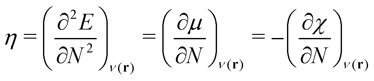
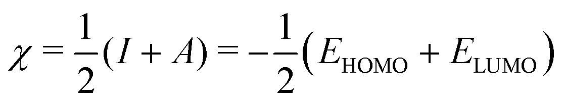
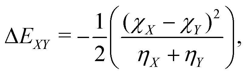
In this section, we summarize main concepts from the conceptual DFT of solutions. The reader is referred to ref. 27, 28 and 32–35 for more details. In addition, we discuss the main ideas of SHAP and ELI5 values in combination with Gini importance criteria.2.1 Conceptual DFT of solutions
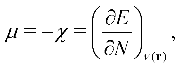 | (1) |
As a prerequisite for chemical reactions, the energy change of isolated molecules upon electronic perturbation can be written as a truncated Taylor series according to
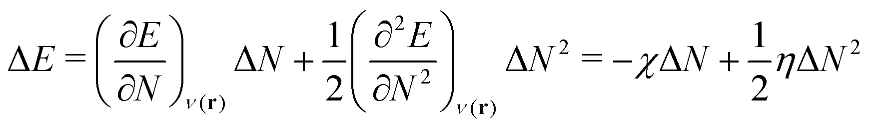 | (2) |
 | (3) |
 | (4) |
| η ≃ I − A = ELUMO − EHOMO, | (5) |
| AS + BS ⇌ (A·B)S | (R1) |
 | (6) |
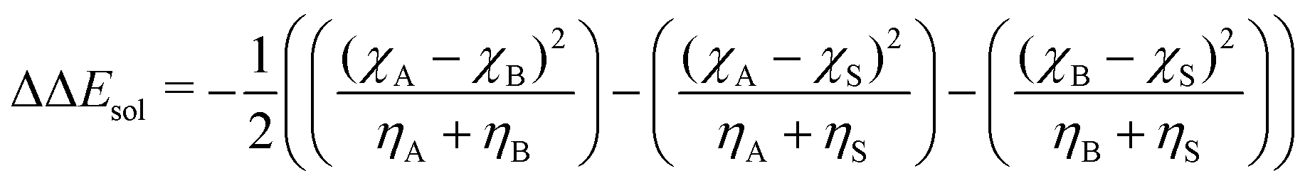 | (7) |
2.2 Explainable machine learning
SHAP value analysis as introduced by Lundberg and Lee12 closely relies on Shapley values as known from game theory.57 In short, Shapley values aim to find a solution on how to distribute the gain or pay-out of a game equally among the players.1 In this context, the main purpose of SHAP analysis is to rationalize a specific value by computing the contribution of each feature to the prediction. The feature values of a data instance can be interpreted as players in a coalition game. In more detail, SHAP values can be written as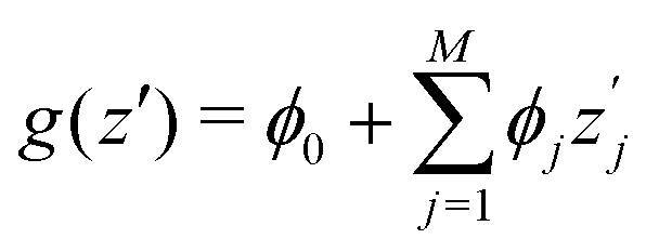 | (8) |
 is the SHAP value.1 Hence, it can be concluded that features with large ϕj values are more important than others. Global SHAP feature importance analysis follows the relation
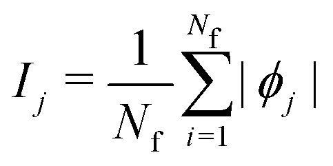 | (9) |
The Gini importance value is a statistical measure to estimate the inequality of a distribution. The concept is widely applied for decision-tree based machine learning approaches. Here, the Gini coefficient estimates the weighted amount of a feature by the number of samples used to split a node into different trees.58 It typically takes values between 0 and 1, so a value of 1 can be interpreted as only one corresponding feature being important for all splits in the decision tree.
ELI5 can be considered as a feature reduction and permutation method.14 Thus, the validated model is iteratively reduced in terms of the individual features and the predictive accuracy is computed. With regard to this approach, one can identify the most important features from a gobal analysis point of view.
3 Numerical and experimental details
3.1 Data sets and considered features
As input training and validation data, we use already published literature and computational results for various ion pairs in distinct protic and aprotic solvents. The corresponding experimental values19,59,60 for the free solvation energies, enthalpies and entropies are used as target values for the machine learning models. The corresponding values of solvents and ions were already published in ref. 33. The training and validation data set59 consisted of 209 entries including different combinations of alkali and halide ions, perchlorate anions, formate (methanoate) anions, methylammonium and ethylammonium in combination with the corresponding solvents dimethyl formamide (DMF), dimethyl sulfoxide (DMSO), ethanol (EtOH), formamide (FA), acetonitrile (MeCN), methanol (MeOH), propylene carbonate (PC) and water. A detailed list of all values and entries can be found in ref. 45. As main features, we used the electronic properties as well as expressions from the conceptual DFT approach. Here, we mainly rely on the computed half-reaction energies (eqn (6)) between the cations and the solvent ΔECS, between the anions and the solvent ΔEAS and between the cations and the anions ΔECA as well as the difference in the cation and anion solvation energies ΔΔEASCS = ΔEAS − ΔECS, the sum of the cation and anion solvation energies ΣΔEASCS = ΔEAS + ΔECS and the corresponding solvation energies in accordance with eqn (7). In addition, we computed the HOMO and LUMO energies as well as the electronegativities and chemical hardnesses of all considered species. Explainable machine learning as well as Gini importance criteria are intended to shed more light on the underlying feature importances. With these approaches, it is usually intended to transform black box models into white box models with known feature-target correlations. In fact, feature pre-selection is usually avoided for these reasons, such that only the model output values are studied and analyzed on their main contributions. In consequence, feature importance analysis is usually performed a posteriori. Therefore, all models trained for different target values are grounded on the same features and an identical training data set. Herewith, we are able to evaluate the feature importances without any hidden knowledge.Thus, we took all chemical reactivity descriptors and derived values as features from the conceptual density functional theory of solutions into consideration.27 In addition, using the differences in the cation- and anion solvation energies as features is motivated by recent experimental studies on the law of matching solvent affinities.24 Such an approach allows us to predict the corresponding free energies, enthalpies and entropies for new solvent-salt combinations even without any experimental values and a priori knowledge. All values can be computed from standard DFT calculations, such that our approach is also broadly applicable for the identification of beneficial new solvent–salt cominations. In consequence, we chose these features according to our theoretical models of charge transfer and solvation, since we have provided ample evidence that these quantities can be used to rationalize solvation processes.27 The corresponding correlation coefficients between the individual features are shown in the ESI.†
3.2 Quantum chemical calculations
The values for the electronegativity, the chemical hardness, the frontier molecular orbital energies and the reaction energies were computed by standard DFT calculations for isolated and geometry-optimized species in the gas phase with the software package Orca 4.0.0.2.61,62 The individual molecular and ionic species were optimized at the DFT level of theory using the B3LYP functional63 in combination with the def2-TZVP64 basis set as used in previous publications.32,33 All calculations utilized an atom-pairwise dispersion correction with the Becke–Johnson damping scheme.65,663.3 Machine learning
As computational regression approaches, we used standard linear regression (LR), linear ridge regression (RID),67 linear Lasso regression (LAS),68 least-angle regression (LARS),69 Bayesian ridge regression (BRID),70 passive-agressive regression (PAR),71 elastic nets (ELN),72 partial-least squares regression of second order (PLS2),73 random forests (RF),74 extra trees (ET),75 support vector machines (SVM),76 gradient boosting (GB) and extreme gradient boosting (XGB),77–79 Gaussian process regression (GP),80,81 Adaboost regression (ADA),82 bagging regression (BAG),83 histogram gradient boosting (HGB)84 and decision trees (DT).85,86 The source code was written in Python 3.9.187 in combination with the modules NumPy 1.19.5,88 scikit-learn 1.0.1,89 XGBoost 1.6.0,90 Pandas 1.2.191 and SHAP 0.40.0.12 If not noted otherwise, all methods were used with default values.4 Results
4.1 Accuracy of model predictions
We start this section with an evaluation of the model accuracy for the ΔGsol, ΔHsol and ΔSsol predictions. For this purpose, we performed a leave-one-out validation approach for all permutations of the training data set and calculated the mean value of the RMSE for all predictions.92 The corresponding results are shown in Fig. 1. The mean RMSE values across all models are RMSE = (11.50 ± 4.51) kJ mol−1 for ΔGsol, RMSE = (9.79 ± 3.50) kJ mol−1 for ΔHsol and RMSE = (35.18 ± 21.43) J K−1 mol−1 for ΔSsol. For the purpose of a better comparability, we introduce the normalized RMSE (nRMSE) value according to | (10) |
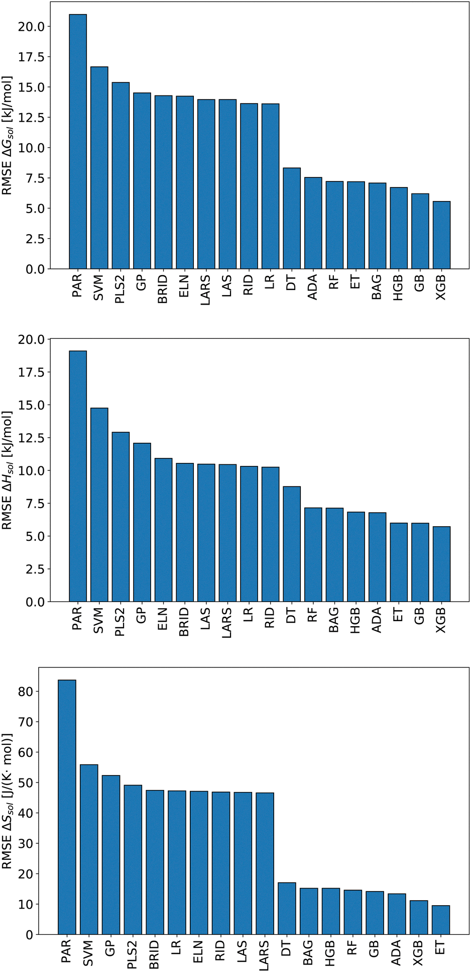 | ||
| Fig. 1 Root-mean-squared error (RMSE) of predicted ΔGsol (top panel), ΔHsol (middle panel) and ΔSsol (bottom panel) after a leave-one-out (LOO) permutation approach for each data point in accordance with different machine learning methods. | ||
Potential reasons for this observation were recently discussed in ref. 93. In more detail, decision-tree based models do not overly smooth the solution in terms of predicted target values. Most other machine learning models such as artificial neural networks (ANNs) transform the training data by smoothing the output with a kernel function like a Gaussian kernel for varying length-scale values. This reduces the impact of irregular patterns for the accurate learning of the predictive function. For small length scales, smoothing the target function on the training set significantly reduces the accuracy of tree-based models but hardly impacts that of ANNs. Moreover, it was shown that uninformative features do not affect the performance metrics of decision-tree based models as much as for other machine learning approaches. In terms of such findings, it becomes clear that decision-tree based models often outperform kernel-based approaches in terms of predictive accuracies.
The detailed predictions in terms of the best model are shown in Fig. 2. For all predictions, one can observe a maximum nRMSE value of 0.22 which demonstrates the high accuracy of all models. Most of the predicted values are located within one σ, such that one can notice only one outlier value related to ΔGsol with an RMSE > 2σ.
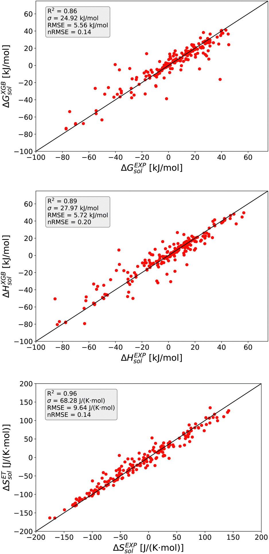 | ||
| Fig. 2 Goodness of fit plots for predicted and experimental values (subscript EXP): XGB model for ΔGsol (top), XGB model for ΔHsol (middle) and ET model for ΔSsol (bottom). The straight black lines highlight a full coincidence. | ||
In more detail, all larger nRMSE deviations with nRMSE > 1.2 for ΔGsol can be attributed to LiBr in PC (nRMSE = 1.50), LiCl in water (nRMSE = 1.65), LiI in PC (nRMSE = 1.28), CsF in methanol (nRMSE = 1.21) and LiF in methanol (nRMSE = 2.22). Thus, it can be concluded that predictions for highly polar solvents including the ions Li+ and F− are more challenging when compared to other combinations of species. Comparable conclusions can also be drawn for some outliers related to ΔHsol predictions. The two outliers with nRMSE > 1.2 can be attributed to LiI in acetonitrile (nRMSE = 1.25) and LiCl in PC (nRMSE = 1.56). With regard to these slight deviations, it was already discussed that fluoride and lithium ions differ from simple charge transfer assumptions which can be rationalized by the small size of the ions and the resulting low polarizability.33
Based on these values, one can conclude that the chosen features from our conceptual DFT approach allow us to predict key thermodynamic values with reasonable accuracy. Noteworthy, the highest accuracy is achieved for the ET model and the corresponding predictions for the solvation entropy. Such findings become even more important with regard to the fact that the conceptual DFT approach for solutions ignores all solution, bulk thermodynamic and multicomponent effects. For a more detailed understanding, we evaluated the individual models in terms of their feature importances.
4.2 Explainable machine learning: feature importances
For an analysis of feature importances, we chose the best models with the highest predictive accuracies shown in Fig. 2 and computed the respective Gini importance values. The corresponding results are shown in Fig. 3. As can be seen, predictions of the XGB model for ΔGsol and ΔSsol are strongly dominated by ΔΔEASCS with Gini values larger than 0.35. A significant drop of feature importances can be observed for the second and third most important features ΔECS and ΣΔEASCS for ΔHsol and ΔECS and ELUMOsol for ΔHsol. The importance of further features for predictions of ΔHsol is nearly negligible while ΔΔEsol and ΔEAS slightly affect the predictions for ΔGsol. In contrast to the XGB models, the dominance of only one feature for predictions of ΔSsol with the ET model is less pronounced. As becomes obvious, the most important features are ηS, followed by ESHOMO and χS. When compared to the feature importances of ΔGsol and ΔHsol, it is evident that predictions for the solvation entropy rely on a broader number of important features. Such findings provide a rationale for the higher accuracy of the ET model, so that a larger number of relevant features also enables more robust predictions.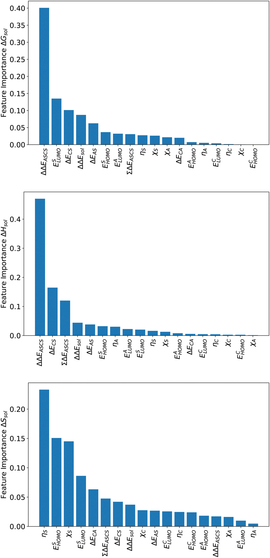 | ||
| Fig. 3 Gini feature importance values from the best models with the highest predictive accuracy. Top: Gini feature importance analysis of the XGB model for the prediction of ΔGsol. Middle: Gini feature importance analysis of the XGB model for the prediction of ΔHsol. Bottom: Gini feature importance analysis of the ET model for the prediction of ΔSsol. | ||
Corresponding conclusions can also be drawn for the net SHAP values as shown in Fig. 4. The features with the highest SHAP values and thus the highest importance are identical with the Gini importance criteria for all three models. Notably, one can observe slight differences in the ordering of the remaining features. In more detail, the frontier molecular orbitals are located at the second and third rank for the predictions of ΔGsol, while ESHOMO also becomes important with regard to the predictions for ΔHsol. In addition to the net SHAP and the Gini importance values, the corresponding ELI5 importance values are presented in Table 1. As can be seen, the most important features like ΔΔEASCS for predictions of ΔGsol and ΔHsol and ηS for predictions of ΔSsol are identical for all analysis methods. Slight differences can be observed for the remaining features. With regard to the rather low Gini, SHAP and ELI5 values for these features and the dominance of the most important feature, the slight discrepancies in terms of different ranking positions become understandable. Hence, clear conclusions on the importance can only be drawn for the most important features. Whereas the comparison between SHAP, ELI5 and Gini values allows us to estimate the net influence of features, the detailed evaluation of SHAP values as shown in Fig. 5 also provides the identification of the functional correlations.
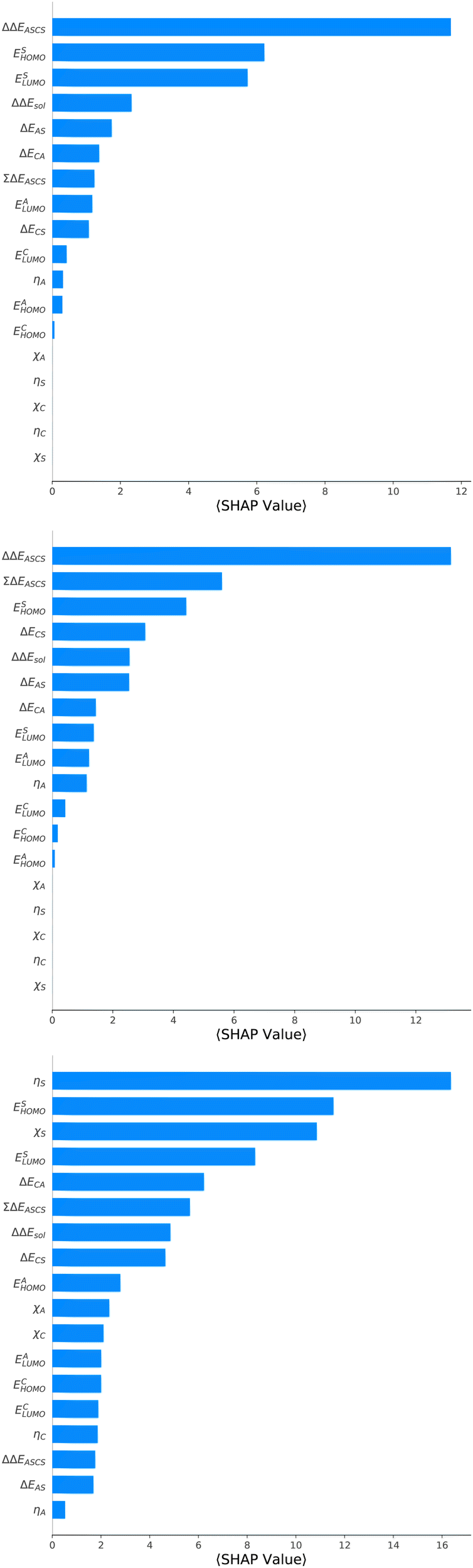 | ||
| Fig. 4 Mean SHAP values for features of the best models. Top: SHAP values for the prediction of ΔGsol (XGB). Bottom: SHAP values for the prediction of ΔHsol (XGB). Bottom: SHAP values for the prediction of ΔSsol (ET). | ||
| Feature | XGB ΔGsol | XGB ΔHsol | ET ΔSsol |
|---|---|---|---|
| ΔΔEASCS | 0.3852 (1) | 0.4709 (1) | 0.0189 (13) |
| E SLUMO | 0.1629 (2) | 0.0226 (10) | 0.0896 (4) |
| E SHOMO | 0.1320 (3) | 0.0681 (4) | 0.1698 (2) |
| ΔECA | 0.0771 (4) | 0.0183 (12) | 0.0490 (6) |
| E ALUMO | 0.0633 (5) | 0.0599 (6) | 0.0117 (17) |
| ΔΔEsol | 0.0553 (6) | 0.0287 (9) | 0.0430 (7) |
| ΔEAS | 0.0378 (7) | 0.0353 (8) | 0.0297 (9) |
| E CLUMO | 0.0265 (8) | 0.0669 (5) | 0.0266 (11) |
| ΣΔEASCS | 0.0174 (9) | 0.0794 (3) | 0.0619 (5) |
| η A | 0.0166 (10) | 0.0909 (2) | 0.0056 (18) |
| E AHOMO | 0.0152 (11) | 0.0378 (7) | 0.0170 (15) |
| ΔECS | 0.0073 (12) | 0.0198 (11) | 0.0401 (8) |
| E CHOMO | 0.0034 (13) | 0.0013 (13) | 0.0181 (14) |
| χ A | 0 (14) | 0 (14) | 0.0154 (16) |
| η S | 0 (15) | 0 (15) | 0.1998 (1) |
| χ C | 0 (16) | 0 (16) | 0.0271 (10) |
| η C | 0 (17) | 0 (17) | 0.0235 (12) |
| χ S | 0 (18) | 0 (18) | 0.1532 (3) |
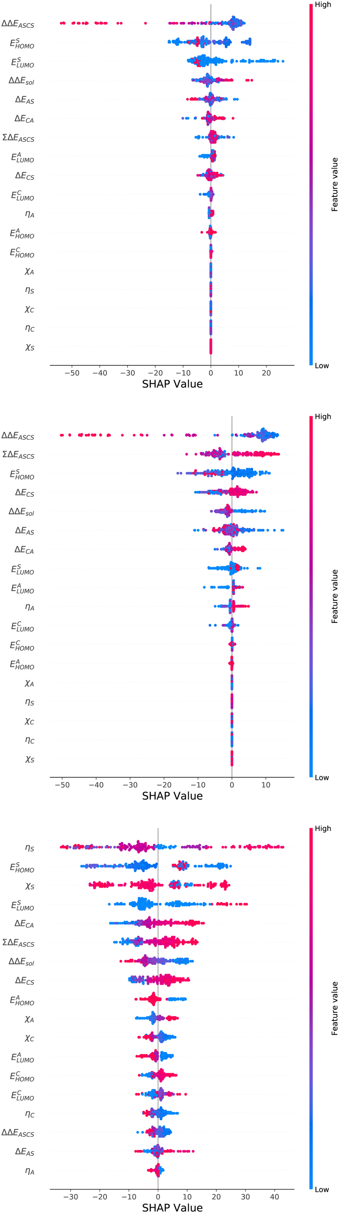 | ||
| Fig. 5 Detailed SHAP values with high (red) and low (blue) feature values for all features in the best models. Top: SHAP values for the XGB model for the prediction of ΔGsol. Bottom: SHAP values for the XGB model for the prediction of ΔHsol. Bottom: SHAP values for the ET model for the prediction of ΔSsol. | ||
With regard to the predictions of ΔGsol for the XGB model, it can be seen that high values of ΔΔEASCS are correlated with negative SHAP values and vice versa. Hence, it can be concluded that high ΔΔEASCS values have a strong positive impact on model predictions. The correlations between high and low values of ESHOMO and ESLUMO with negative and positive SHAP values are less obvious. For high values of these features, one can observe at least a clear separation between positive and negative SHAP values. In addition, the values for the solvation energy show a reasonable positive correlation, such that high values are correlated with positive SHAP values and vice versa. This correlation is not surprising, as the solvation energy was introduced with the main intention to compute thermodynamic solvation energies.
A comparable outcome in terms of antilinear correlations for ΔΔEASCS can also be observed for the model predictions of ΔHsol. Moreovoer, one can observe that ΣΔEASCS shows a positive correlation between high values and positive SHAP values. The remaining features show a rather ambiguous correlation. Also the SHAP values for the model predictions of ΔSsol show no clear trends. However, it has to be noted that high values of χS lead to negative SHAP values and thus lower values of ΔSsol. Corresponding clear correlations can also be seen for ESLUMO, where low values lead to negative SHAP values. Notably, the most important feature ηS shows a rather ambiguous distribution of low and high values in terms of corresponding SHAP values. As can be seen, the standard deviations for all features in terms of the corresponding SHAP values are significantly broader when compared to the other models. The individual interpretation of these contributions is discussed in the next subsection.
Furthermore, we performed additional calculations for the same training data and models but with reduced feature sets. In more detail, we ignored the most important feature from the SHAP analysis for all considered models. The corresponding results are shown in the ESI.† As can be seen, the predictions for the reduced models slightly change. For the free energy of solvation it becomes clear that the prediction accuracy decreases slightly. In addition, the most important feature is now the cation–solvent solvation energy. This finding is valid for all three reduced models and accordingly for the predictions for the solvation free energy, enthalpy, and entropy, and can be explained by the large energetic differences between the solvent and the cation. Accordingly, the solvation energies of these species dominate the feature set. Only for the predictions of the free enthalpy a slight increase in the prediction accuracy after reduction of the feature set can be observed, while the results for the free entropy of solvation show a lower prediction accuracy. Therefore, one cannot conclude that by ignoring the most important feature, the second most important feature automatically becomes dominant. In addition, it can be seen that reducing the feature space for the most important contributor most often decreases the prediction accuracy. Since one is usually not aware of the relevant characteristics beforehand, such a manual check is definitely not useful, as it introduces a bias. Accordingly, these feature set results highlight the nonlinear correlations between the input features and the output target values.
4.3 Interpretation of feature importances
As outlined in the previous subsection, the predictions for the free solvation energy and solvation enthalpy are dominated by a few features while the entropy predictions rely on different pillars. With regard to the individual ΔGsol and ΔHsol model predictions, it becomes obvious that both models are strongly dominated by ΔEASCS. A recent publication34 discusses the importance of this parameter with regard to thermodynamic principles in the context of specific ion effects and volcano plots.59 In more detail, it was shown for the ‘law of matching solvent affinities’22,24 that species with vanishing ΔEASCS reveal a strong ion pairing tendency as underlined by positive ΔHsol values. Such experimental findings can be understood in terms of the 'strong and weak acids and bases' (SWAB) principle,33 which states that ions with comparable electronegativity differences show vanishing ΔEASCS values. In consequence, the dominance of this feature in the model predictions for ΔGsol and ΔHsol is a direct consequence of the underlying specific ion effects and the validity of the conceptual DFT approach for solutions.28,34 Moreover, the lower importance of ΔΔEsol and ΔECA can be rationalized by the complex nature of ion pairs. In contrast to covalently bound products, ion pairs show a range of different conformations. One can distinguish between direct contact ion pairs, solvent-shared ion pairs, solvent-mediated ion pairs and ion aggregates.18 The corresponding binding energies associated with the individual states often differ significantly. Hence, depending on the ion species in combination with the chosen solvent, it is often not clear which ion pairing state dominates. Thus, the exact values for the solvation energy as well as the ion binding energy are often not that well defined, such that the features representing these energies show a lower importance on the model outcomes.Further conclusions can also be drawn for the importance of ESHOMO and ESLUMO in terms of predictions for ΔGsol. Notably, the corresponding frontier molecular orbital energies can be interpreted as vertical electron affinity and ionization potential of solvent molecules which thus point to charge redistribution effects upon interaction.37 As was recently discussed,32,34 charge transfer is an essential contribution to solvation interactions and the formation of solvation bonds. In consequence, the HOMO and LUMO energies are pointing to the importance of the electronic solvation properties for solvents as also discussed in the context of donor and acceptor numbers.20,28,32 Based on these findings, we conclude that the predictions for the free solvation energy and enthalpy are highly dominated by the electronic properties of the solvent. Such assumptions were already discussed in the conceptual DFT approach for solutions26 and the corresponding results of our analysis fully validate this concept. Despite the fact that conceptual DFT calculations show some slight deviations to experimental results due to crucial approximations, we showed that the underlying framework reflects a reasonable qualitative agreement in terms of highly accurate model predictions in combination with the corresponding feature analysis.
A slightly different conclusion can be drawn for the model analysis of solvation entropy predictions. The high accuracy of the predictions is remarkable with regard to the fact that only the electronic properties of the molecules in combination with solvation energies are taken into consideration. Hence, further potentially important features reflecting bulk thermodynamic properties, the composition of the solution as well as environmental factors like temperature and pressure are not considered in our models. As can be seen, the most important features ηS, ESHOMO and χS for the model predictions are strongly related to the electronic properties of the solvent molecules. Notably, solvation entropies are crucially dominated by the local arrangement of the species in the solution in combination with kinetic restrictions.19 As already discussed, the chemical hardness of the solvent as the most relevant feature is an inverse measure for the polarizability α. It was recently shown that larger molecules usually reveal lower chemical hardnesses and thus higher polarizabilities.27 One can thus assume that the importance of this feature for the model predictions points to the impact of the size and strength of molecular interactions between the solute species and the solvent molecules. Hence, it can be assumed that the thermodynamic solvation entropy is crucially affected by the electronic properties of the solvent molecules. As already known, molecules with varying polarizabilities differ in their position and their orientation around solute species.26 In addition, it was shown that the polarizabilities also affect the dipole moment which thus influences the orientation of the solvent molecules around the solute species. Furthermore, the influence of the solvent HOMO energy ESHOMO can also be interpreted as an influence of the ionization potential, whereby this feature describes the electron donating properties of the solvent. As already shown in earlier publications,32,35 this behavior can also be classified by the donor numbers, which allow the binding energies of the solvent to be estimated accordingly. In consequence, different binding strengths can also be translated into different flexible local orientations of the solvent molecules around the solute species as well as differences in the dynamic binding times. Comparable conclusions can also be drawn for the electronegativity χS, which estimates the Lewis acidity or basicity of the solvent molecules. With regard to previous discussions,34 it can be concluded that these properties of the solvent play an important role for certain SWAB principles and thus provide an estimate for the strength of cation–anion interactions as well as the individual solvation energies between the solvent molecules and the ions. Notably, it was proven94 that the HSAB principle can be derived from the “|Δμ| big is good” (DMB) rule. In a recent paper, we were also able to show that the SWAB principles can be derived from the DMB condition.95 Hence, one can conclude that the SWAB and the HSAB principles are closely connected to the DMB condition which is known as a cardinal reactivity principle. In summary, it can be concluded that the electronic properties of the solvent molecules as well as their polarizability play an important role for the resulting entropy values in terms of distinct ion pair solvent combinations.
5 Summary and conclusion
In this article, we combined conceptual DFT with explainable machine learning approaches for highly accurate model predictions of certain thermodynamic solvation parameters in combination with the analysis of feature importances. The results of our calculations showed a high accuracy for the prediction of the free solvation energy, the solvation enthalpy and the solvation entropy. The corresponding correlation coefficients between predicted and experimental validation values are for the best models higher than R2 = 0.86 with a maximum nRMSD of 0.22. Notably, the most accurate predictions were obtained for decision-tree based models which shows the highly non-linear contribution of different features on the solvation thermodynamics. Notable deviations from the experimental values were only observed for Li+ ions in combination with highly polar solvents. It was recently discussed that lithium ions behave differently when compared to all the other alkali ions which rationalizes these findings.96The high accuracy of the machine learning methods allowed us to shed light on the most important features. The corresponding results for the free solvation energy and enthalpy highlighted a prominent influence of the differences in the solvation energies for the cations and the anions. These findings are in reasonable agreement with recent discussions in terms of the ‘law of matching solvent affinities’.23,24 This concept can be generalized to the SWAB principle, which states that ions with comparable electronegativity differences to the solvent form the strongest ion pairs with the highest solvation enthalpies.32–34 Thus, one can directly conclude from our feature analysis that this principle governs the solvation of ion pairs in solution as the most important parameter. Moreover, we have shown that the ionization potential and the electron affinity of the solvent further dominate the solvation enthalpies and energies. Such results can be brought into relation with recent discussions about solvent influences and the role of donor and acceptor numbers which further provide the identification of reasonable solvent–ion combinations.28,32
Finally, it should be noted that even entropies of solvation can be predicted with high accuracy in terms of the conceptual DFT approach. In more detail, solvation entropies are bulk thermodynamic properties which rely on the composition, orientation and dynamics of the species in solution. Our explainable machine learning approach unraveled the reasons for the high accuracy of the predictions. In more detail, the chemical hardness, the HOMO energy as well as the electronegativity of the solvent play a key role. The chemical hardness can be interpreted as an inverse polarizability which can be attributed to the molecular size of the solvent species. It was discussed that differences in the solvent molecular size and shape crucially affect the solution entropies.19 Corresponding conclusions are also valid for all electron-donating or accepting properties of solvents in terms of electronegativity values. The pronounced importance of these effects highlights the crucial role of local intermolecular interactions in terms of charge transfer mechanisms. The outcomes of our explainable machine learning analysis thus validate recent theoretical assumptions.26–28,32–35
Our results show that explainable machine learning approaches in combination with theoretical frameworks provide deeper insights into fundamental principles. In addition to accurate predictions, one can analyze the main features with the highest importance which gives insights into the dominant contributions and governing mechanisms. In consequence, it can be concluded that the viable combination of machine learning methods with experimental data, theoretical considerations and feature importance analysis may lead to the exploration of unknown relations and a deeper understanding of correlations. These conclusions are not unique to our study, so they can be generalized to all aspects of science where a reasonable amount of data, highly predictive models, and some basic knowledge of relationships and feature meanings are available.
Conflicts of interest
All authors except RAMQ are employees of Boehringer Ingelheim.Acknowledgements
The authors thank Virginia Mazzini, Vince S. J. Craig, Volker Tittelbach-Helmrich, Kerstin Schäfer, Moritz Schulze, Huayu Li, Robert Möckel and Victor Emenike for valuable discussions and useful hints. RAMQ thanks the University of Florida for funding this work in terms of a start-up grant.Notes and references
- C. Molnar, Interpretable machine learning, Lulu.com, 2020.
- W. J. Murdoch, C. Singh, K. Kumbier, R. Abbasi-Asl and B. Yu, Proc. Natl. Acad. Sci. U. S. A., 2019, 116, 22071–22080 CrossRef CAS PubMed.
- M. Du, N. Liu and X. Hu, Commun. ACM, 2019, 63, 68–77 CrossRef.
- C. Molnar, G. Casalicchio and B. Bischl, Joint European Conference on Machine Learning and Knowledge Discovery in Databases, 2020, pp. 417–431 Search PubMed.
- F. Doshi-Velez and B. Kim, arXiv, 2017, preprint, arXiv:1702.08608 DOI:10.48550/arXiv.1702.08608.
- P. Linardatos, V. Papastefanopoulos and S. Kotsiantis, Entropy, 2020, 23, 18 CrossRef PubMed.
- V. Belle and I. Papantonis, Front. Big Data, 2021, 4, 688969 CrossRef PubMed.
- B. Kailkhura, B. Gallagher, S. Kim, A. Hiszpanski and T. Han, npj Comput. Mater., 2019, 5, 1–9 CrossRef.
- A. Holzinger, P. Kieseberg, E. Weippl and A. M. Tjoa, International Cross-Domain Conference for Machine Learning and Knowledge Extraction, 2018, pp. 1–8.
- D. Gunning, M. Stefik, J. Choi, T. Miller, S. Stumpf and G.-Z. Yang, Sci. Robot., 2019, 4, 7120 CrossRef PubMed.
- B. Sudret, Reliabil. Eng. Sys. Safety, 2008, 93, 964–979 CrossRef.
- S. M. Lundberg and S.-I. Lee, A unified approach to interpreting model predictions, Advances in Neural Information Processing Systems, 2017, vol. 30 Search PubMed.
- M. T. Ribeiro, S. Singh and C. Guestrin, Model-Agnostic Interpretability of Machine Learning, arXiv, 2016, preprint, arXiv:1606.05386 DOI:10.48550/arXiv.1606.05386.
- N. Agarwal and S. Das, 2020 IEEE Symposium Series on Computational Intelligence (SSCI), 2020, pp. 1528–1534.
- N. Artrith, K. T. Butler, F.-X. Coudert, S. Han, O. Isayev, A. Jain and A. Walsh, Nat. Chem., 2021, 13, 505–508 CrossRef CAS PubMed.
- J. P. Janet and H. J. Kulik, Machine Learning in Chemistry, American Chemical Society, 2020 Search PubMed.
- G. Carleo, I. Cirac, K. Cranmer, L. Daudet, M. Schuld, N. Tishby, L. Vogt-Maranto and L. Zdeborová, Rev. Mod. Phys., 2019, 91, 045002 CrossRef CAS.
- J. Smiatek, A. Heuer and M. Winter, Batteries, 2018, 4, 62 CrossRef CAS.
- Y. Marcus, Ions in Solution and their Solvation, John Wiley & Sons, 2014 Search PubMed.
- C. Reichardt and T. Welton, Solvents and Solvent Effects in Organic Chemistry, John Wiley & Sons, 2011 Search PubMed.
- Y. Marcus, Chem. Rev., 2009, 109, 1346–1370 CrossRef CAS PubMed.
- K. D. Collins, Biophys. J., 1997, 72, 65 CrossRef CAS PubMed.
- K. P. Gregory, G. Elliott, H. Robertson, A. Kumar, E. J. Wanless, G. B. Webber, V. S. Craig, G. G. Andersson and A. Page, Phys. Chem. Chem. Phys., 2022, 24, 12682–12718 RSC.
- V. Mazzini and V. S. Craig, ACS Cent. Sci., 2018, 4, 1056–1084 CrossRef CAS PubMed.
- V. Mazzini and V. S. Craig, Curr. Opin. Colloid Interface Sci., 2016, 23, 82–93 CrossRef CAS.
- R. A. Miranda-Quintana and J. Smiatek, J. Phys. Chem. B, 2021, 125, 11857–11868 CrossRef CAS PubMed.
- R. A. Miranda-Quintana and J. Smiatek, J. Phys. Chem. B, 2021, 125, 13840–13849 CrossRef CAS PubMed.
- R. A. Miranda-Quintana and J. Smiatek, Electrochim. Acta, 2021, 384, 138418 CrossRef CAS.
- A. Ben-Naim, Statistical thermodynamics for chemists and biochemists, Springer Science & Business Media, Berlin, Germany, 2013 Search PubMed.
- A. Ben-Naim, Solvation thermodynamics, Springer Science & Business Media, 2013 Search PubMed.
- J. Smiatek, Molecules, 2020, 25, 1661 CrossRef CAS PubMed.
- J. Smiatek, J. Chem. Phys., 2019, 150, 174112 CrossRef PubMed.
- J. Smiatek, J. Phys. Chem. B, 2020, 124, 2191–2197 CrossRef CAS PubMed.
- R. A. Miranda-Quintana and J. Smiatek, ChemPhysChem, 2020, 21, 2605 CrossRef CAS PubMed.
- R. A. Miranda-Quintana and J. Smiatek, J. Mol. Liquids, 2021, 322, 114506 CrossRef CAS.
- P. Geerlings, E. Chamorro, P. K. Chattaraj, F. De Proft, J. L. Gázquez, S. Liu, C. Morell, A. Toro-Labbé, A. Vela and P. Ayers, Theo. Chem. Acc., 2020, 139, 1–18 CrossRef.
- P. Geerlings, F. De Proft and W. Langenaeker, Chem. Rev., 2003, 103, 1793–1873 CrossRef CAS PubMed.
- P. K. Chattaraj, S. Utpal and D. R. Roy, Chem. Rev., 2006, 106, 2065–2091 CrossRef CAS PubMed.
- R. G. Parr and R. G. Pearson, J. Am. Chem. Soc., 1983, 105, 7512–7516 CrossRef CAS.
- H. Chermette, J. Comput. Chem., 1999, 20, 129–154 CrossRef CAS.
- P. W. Ayers, J. Chem. Phys., 2005, 122, 141102 CrossRef PubMed.
- P. W. Ayers, R. G. Parr and R. G. Pearson, J. Chem. Phys., 2006, 124, 194107 CrossRef PubMed.
- P. W. Ayers, Faraday Discuss., 2007, 135, 161–190 RSC.
- J. L. Gázquez, J. Mex. Chem. Soc., 2008, 52, 3–10 Search PubMed.
- J. Yang, M. J. Knape, O. Burkert, V. Mazzini, A. Jung, V. S. Craig, R. A. Miranda-Quintana, E. Bluhmki and J. Smiatek, Phys. Chem. Chem. Phys., 2020, 22, 24359–24364 RSC.
- R. G. Parr, R. A. Donnelly, M. Levy and W. E. Palke, J. Chem. Phys., 1978, 68, 3801–3807 CrossRef CAS.
- P. K. Chattaraj, H. Lee and R. G. Parr, J. Am. Chem. Soc., 1991, 113, 1855–1856 CrossRef CAS.
- R. A. Miranda-Quintana, J. Chem. Phys., 2017, 146, 046101 CrossRef PubMed.
- P. K. Chattaraj and S. Giri, Annu. Rep. Phys. Chem., 2009, 105, 13–39 RSC.
- J. F. Janak, Phys. Rev. B: Condens. Matter Mater. Phys., 1978, 18, 7165 CrossRef CAS.
- T. Koopmans, Physica, 1934, 1, 104–113 CrossRef.
- R. A. Miranda-Quintana and P. W. Ayers, Phys. Chem. Chem. Phys., 2016, 18, 15070–15080 RSC.
- R. S. Mulliken, J. Chem. Phys., 1934, 2, 782–793 CrossRef CAS.
- R. A. Miranda-Quintana and P. W. Ayers, J. Chem. Phys., 2018, 148, 196101 CrossRef PubMed.
- R. A. Miranda-Quintana and P. W. Ayers, Theo. Chem. Acc., 2019, 138, 44 CrossRef.
- R. A. Miranda-Quintana, Theor. Chem. Acc., 2017, 136, 76 Search PubMed.
- L. Shapley, Contributions to the Theory of Games, 1953, p. 343 Search PubMed.
- T. Daniya, M. Geetha and K. S. Kumar, Adv. Math. Sci. J., 2020, 9, 1857–8438 Search PubMed.
- V. Mazzini, G. Liu and V. S. Craig, J. Chem. Phys., 2018, 148, 222805 CrossRef PubMed.
- Y. Marcus and G. Hefter, Chem. Rev., 2006, 106, 4585–4621 CrossRef CAS PubMed.
- F. Neese, Wiley Interdiscip. Rev.: Comput. Mol. Sci., 2012, 2, 73–78 CAS.
- F. Neese, Wiley Interdiscip. Rev.: Comput. Mol. Sci., 2018, 8, e1327 Search PubMed.
- C. Lee, W. Yang and R. G. Parr, Phys. Rev. B: Condens. Matter Mater. Phys., 1988, 37, 785 CrossRef CAS PubMed.
- F. Weigend and R. Ahlrichs, Phys. Chem. Chem. Phys., 2005, 7, 3297–3305 RSC.
- S. Grimme, J. Antony, S. Ehrlich and H. Krieg, J. Chem. Phys., 2010, 132, 154104 CrossRef PubMed.
- S. Grimme, S. Ehrlich and L. Goerigk, J. Comput. Chem., 2011, 32, 1456–1465 CrossRef CAS PubMed.
- G. C. McDonald, Wiley Interdiscip. Rev.: Comput. Mol. Sci., 2009, 1, 93–100 CrossRef.
- J. Ranstam and J. Cook, J. Brit. Surg., 2018, 105, 1348 CrossRef.
- B. Efron, T. Hastie, I. Johnstone and R. Tibshirani, Ann. Stat., 2004, 32, 407–499 Search PubMed.
- A. G. Assaf, M. Tsionas and A. Tasiopoulos, Tourism Manage., 2019, 71, 1–8 CrossRef.
- K. Crammer, O. Dekel, J. Keshet, S. Shalev-Shwartz and Y. Singer, J. Mach. Learn. Res., 2006, 7, 551–585 Search PubMed.
- H. Zou and T. Hastie, J. Roy. Stat. Soc. B, 2005, 67, 301–320 CrossRef.
- S. Wold, M. Sjöström and L. Eriksson, Chem. Intell. Lab. Sys., 2001, 58, 109–130 CrossRef CAS.
- L. Breiman, Mach. Learn., 2001, 45, 5–32 CrossRef.
- P. Geurts, D. Ernst and L. Wehenkel, Mach. Learn., 2006, 63, 3–42 CrossRef.
- D. A. Pisner and D. M. Schnyer, Machine Learning, Elsevier, 2020, pp. 101–121 Search PubMed.
- L. Mason, J. Baxter, P. Bartlett and M. Frean, Advances in Neural Information Processing Systems, MIT Press, 1999, vol. 12, pp. 512–518 Search PubMed.
- J. H. Friedman, Ann. Stat., 2001, 1189–1232 Search PubMed.
- R. P. Sheridan, W. M. Wang, A. Liaw, J. Ma and E. M. Gifford, J. Chem. Inf. Model., 2016, 56, 2353–2360 CrossRef CAS PubMed.
- M. Seeger, Int. J. Neural Sys., 2004, 14, 69–106 CrossRef PubMed.
- C. K. Williams and C. E. Rasmussen, Gaussian Processes for Machine Learning, MIT press, Cambridge, MA, 2006 Search PubMed.
- M. Collins, R. E. Schapire and Y. Singer, Mach. Learn., 2002, 48, 253–285 CrossRef.
- P. Bühlmann, Handbook of computational statistics, Springer, 2012, pp. 985–1022 Search PubMed.
- R. Blaser and P. Fryzlewicz, J. Mach. Learn. Res., 2016, 17, 126–151 Search PubMed.
- A. J. Myles, R. N. Feudale, Y. Liu, N. A. Woody and S. D. Brown, J. Chemometrics, 2004, 18, 275–285 CrossRef CAS.
- B. Kamiński, M. Jakubczyk and P. Szufel, Cent. Eur. J. Oper. Res., 2018, 26, 135–159 CrossRef PubMed.
- G. Van Rossum and F. L. Drake, Python 3 Reference Manual, CreateSpace, Scotts Valley, CA, 2009 Search PubMed.
- C. R. Harris, K. J. Millman, S. J. van der Walt, R. Gommers, P. Virtanen, D. Cournapeau, E. Wieser, J. Taylor, S. Berg, N. J. Smith, R. Kern, M. Picus, S. Hoyer, M. H. van Kerkwijk, M. Brett, A. Haldane, J. F. del Río, M. Wiebe, P. Peterson, P. Gérard-Marchant, K. Sheppard, T. Reddy, W. Weckesser, H. Abbasi, C. Gohlke and T. E. Oliphant, Nature, 2020, 585, 357–362 CrossRef CAS PubMed.
- F. Pedregosa, G. Varoquaux, A. Gramfort, V. Michel, B. Thirion, O. Grisel, M. Blondel, P. Prettenhofer, R. Weiss, V. Dubourg, J. Vanderplas, A. Passos, D. Cournapeau, M. Brucher, M. Perrot and E. Duchesnay, J. Mach. Learn. Res., 2011, 12, 2825–2830 Search PubMed.
- J. Brownlee, XGBoost With python: Gradient boosted trees with XGBoost and scikit-learn, Machine Learning Mastery, 2016 Search PubMed.
- W. McKinney, Proceedings of the 9th Python in Science Conference, 2010, pp. 56–61.
- T.-T. Wong, Pattern Recogn., 2015, 48, 2839–2846 CrossRef.
- L. Grinsztajn, E. Oyallon and G. Varoquaux, Why do tree-based models still outperform deep learning on tabular data?, arXiv, 2022, preprint, arXiv.2207.08815 DOI:10.48550/arXiv.2207.08815.
- R. A. Miranda-Quintana, T. D. Kim, C. Cárdenas and P. W. Ayers, Theo. Chem. Acc., 2017, 136, 135 CrossRef.
- R. A. Miranda-Quintana and J. Smiatek, J. Phys. Chem. B, 2022, 126, 8864–8872 CrossRef CAS PubMed.
- M. Kohagen, F. Uhlig and J. Smiatek, Int. J. Quantum Chem., 2019, 119, e25933 CrossRef.
Footnote |
| † Electronic supplementary information (ESI) available. See DOI: https://doi.org/10.1039/d2cp04428e |
| This journal is © the Owner Societies 2022 |