
 Open Access Article
 This Open Access Article is licensed under a Creative Commons Attribution-Non Commercial 3.0 Unported Licence
Simulation of the photodetachment spectra of the nitrate anion (NO3−) in the ![[B with combining tilde]](https://www.rsc.org/images/entities/h2_char_0042_0303.gif) 2E′ energy range and non-adiabatic electronic population dynamics of NO3
2E′ energy range and non-adiabatic electronic population dynamics of NO3
David M. G.
Williams
 abc,
Wolfgang
Eisfeld
c and
Alexandra
Viel
*d
abc,
Wolfgang
Eisfeld
c and
Alexandra
Viel
*d
aDepartment of Chemistry and The PULSE Institute, Stanford University, Stanford, California 94305, USA. E-mail: mgw@stanford.edu
bSLAC National Accelerator Laboratory, 2575 Sand Hill Road, Menlo Park, California 94025, USA
cTheoretische Chemie, Universität Bielefeld, Postfach 100131, D-33501 Bielefeld, Germany. E-mail: wolfgang.eisfeld@uni-bielefeld.de
dUniv Rennes, CNRS, IPR (Institut de Physique de Rennes) - UMR 6251, F-35000 Rennes, France. E-mail: alexandra.viel@univ-rennes1.fr
First published on 29th July 2022
Abstract
The photodetachment spectrum of the nitrate anion (NO3−) in the energy range of the NO3 second excited state is simulated from first principles using quantum wave packet dynamics. The prediction at 10 K and 435 K relies on the use of an accurate full-dimensional fully coupled five state diabatic potential model utilizing an artificial neural network. The ability of this model to reproduce experimental spectra was demonstrated recently for the lower energy range [A. Viel, D. M. G. Williams and W. Eisfeld, J. Chem. Phys. 2021, 154, 084302]. Analysis of the spectra indicates a weaker Jahn–Teller coupling compared to the first excited state. The detailed non-adiabatic dynamics is studied by computing the population dynamics. An ultra-fast non-statistical radiationless decay is found only among the Jahn–Teller components, which is followed by a slow statistical non-radiative decay among the different state manifolds. The latter is reproduced perfectly by a simple first order kinetics model. The dynamics in the second excited state is not affected by the presence of a conical intersection with the first excited state manifold.
I. Introduction
The nitrate radical (NO3) in its electronic ground and first two excited states is a prototype of the complex quantum dynamics induced by the Jahn–Teller (JT) effect. For this reason it has been studied for decades both experimentally and theoretically. The theoretical treatment was driven by the development of more and more accurate models for the coupled potential energy surfaces (PESs).1–13 This development was hampered initially by the artificial symmetry-breaking of the electronic wave function, which was discovered and solved in 2000.14,15 Other key steps for the improvement of accuracy were the development of higher-order expansions of the diabatic JT Hamiltonian5,10,16,17 and most recently the use of artificial neural networks (ANNs).13,18–21The ground state of NO3 corresponds to a  state (
![[X with combining tilde]](https://www.rsc.org/images/entities/char_0058_0303.gif) ) with a D3h symmetric equilibrium geometry and the first two excited states transform as 2E′′ (Ã) and 2E′ (
) with a D3h symmetric equilibrium geometry and the first two excited states transform as 2E′′ (Ã) and 2E′ (![[B with combining tilde]](https://www.rsc.org/images/entities/char_0042_0303.gif) ), respectively. The state is easily accessible in direct absorption and thus is known since the 1930s.22,23 By contrast, the à state has a vanishing electric dipole transition moment with respect to the state due to symmetry and thus is not easy to detect. The first photodetachment measurement of this state (starting from the anion NO3−) by Neumark and co-workers in 1991 was a groundbreaking experiment,24 which also triggered theoretical efforts to understand and explain the spectrum. In this spectrum, two bands are seen clearly, corresponding to the and the à state. The state spectrum was simulated early on and quite satisfactorily using a simple vibronic coupling model.1 The theoretical treatment of the à state turned out to be much more demanding.4,5 Finally, good agreement between experiment and theory was obtained in 2014.10 However, these early spectra were comparably hot (≈435 K) and thus there started a debate about certain features whether they are caused by vibronic coupling or are hot bands. Very recently, the Neumark group published a new photodetachment spectrum at cryogenic temperature and with much better resolution.25 Unfortunately, only the state band was detected in the new experiment.
), respectively. The state is easily accessible in direct absorption and thus is known since the 1930s.22,23 By contrast, the à state has a vanishing electric dipole transition moment with respect to the state due to symmetry and thus is not easy to detect. The first photodetachment measurement of this state (starting from the anion NO3−) by Neumark and co-workers in 1991 was a groundbreaking experiment,24 which also triggered theoretical efforts to understand and explain the spectrum. In this spectrum, two bands are seen clearly, corresponding to the and the à state. The state spectrum was simulated early on and quite satisfactorily using a simple vibronic coupling model.1 The theoretical treatment of the à state turned out to be much more demanding.4,5 Finally, good agreement between experiment and theory was obtained in 2014.10 However, these early spectra were comparably hot (≈435 K) and thus there started a debate about certain features whether they are caused by vibronic coupling or are hot bands. Very recently, the Neumark group published a new photodetachment spectrum at cryogenic temperature and with much better resolution.25 Unfortunately, only the state band was detected in the new experiment.
The new experiment and our development of a very accurate full-dimensional diabatic PES model for the , Ã, and electronic states of NO3 was the inspiration for a detailed theoretical study of the band of the photodetachment spectra.13 These quantum dynamics simulations accounted for hot bands of the high-temperature spectra of the state as well as for near threshold effects (Wigner's Threshold Law) affecting the intensity ratios depending on the detachment laser frequency. All these effects were reproduced in excellent agreement with the available experiments at 435 and 10 K. The accuracy of these results allowed for a detailed analysis which effects contribute to the various observed spectral features and to what degree. It was possible to show to which degree vibronic coupling to the state contributes to various features in the band and to distinguish these effects from hot bands. The focus of that study was the NO3 ground state, though the vibronic coupling effects to the two excited à and states fully were accounted for. The focus of the present study is on the excited states dynamics in neutral NO3 after detaching an electron from the anion NO3−. Our latest PES model13 allows for the first time to simulate the photodetachment spectrum of the state, which was observed experimentally together with the and à state.26 Similar negative ion detachment spectra were also measured for the carbon analogue CO3−![[thin space (1/6-em)]](https://www.rsc.org/images/entities/char_2009.gif) 27,28 and sulfur analogue SO3−.29 One of the most interesting aspects when considering the dynamics, initiated by detachment to the second excited state of NO3, is that the state shows a low-lying conical intersection with the à state. According to conventional wisdom, this should cause ultra-fast population decay. Thus, a central aspect of the present study is the investigation of the nonadiabatic population dynamics among the various electronic states of the NO3 radical.
27,28 and sulfur analogue SO3−.29 One of the most interesting aspects when considering the dynamics, initiated by detachment to the second excited state of NO3, is that the state shows a low-lying conical intersection with the à state. According to conventional wisdom, this should cause ultra-fast population decay. Thus, a central aspect of the present study is the investigation of the nonadiabatic population dynamics among the various electronic states of the NO3 radical.
II. Computational details
The time-dependent quantum wave packet propagation is the appropriate choice to compute both photo-detachment spectra and time evolution of electronic populations. To this end, the MCTDH approach,30,31 suitable for the representation of wave functions with large dimensionality is used. More specifically, the propagation of a 6-dimensional wavepacket evolving on the 5 coupled PESs of the radical is performed starting from the eigenfunction of each of the lowest vibrational states of NO3−. The spectra obtained by the Fourier transform of the resulting autocorrelation functions are subsequently added with the proper Boltzmann weights to simulate the NO3− photodetachment spectrum at a given temperature. The determination of the vibrational eigenfunctions of the anion is achieved by the state average and block diagonalization scheme.32 The diabatic and adiabatic populations are obtained via the analysis of the wavepacket. The diabatic populations are read from the wavepacket decomposition in terms of the MCTDH basis. The adiabatic populations are obtained via the CDVR scheme33 and its generalized version as detailed in the appendix of ref. 34.Two kinds of coordinate sets were employed for the dynamics calculations. These are the internal curvilinear coordinates ρ(cu), ϑ(cu), φ(cu), θ(cu), ϕ(cu), χ(cu), as proposed in ref. 35, and the mass weighted normal modes defined at the geometry of the anion potential minimum. It was demonstrated in previous studies11,12 that the curvilinear coordinates and the associated quasi-exact kinetic operator as obtained in ref. 35 provide results of sufficient accuracy when compared to exact computations performed with stereographic coordinates. In the present work, it was found that using normal modes for the computation of electronic population evolutions and thus a simplified kinetic operator are sufficient to obtain the desired accuracy.
The determination of the initial states of the NO3− anion was carried out using a single adiabatic full-dimensional PES published in ref. 10. This PES represents high-level coupled-cluster CCSD(T) calculations with a large atomic orbital basis set (aug-cc-pVQZ plus a set of universal Rydberg functions). The PES is expanded in the invariants in terms of symmetry-adapted internal displacement coordinates to full sixth order. The 132 free parameters were fitted with respect to roughly 1800 data points with a root mean-square error (rmse) of 17 cm−1. The low-lying vibrational eigenstates were computed on this PES and the corresponding energies are reproduced in Table 1 together with the Boltzmann weights evaluated at 435 K. Contributions from the NO3− antisymmetric and symmetric stretching levels are neglected given their Boltzmann weights of less than 5%. The final spectrum at 435 K is thus a sum over four separate wave packet propagations.
Tables 2 and 3 provide the numerical details of the basis set used for the representation of the wave-packets. Careful attention was paid to the definition of the underlying box as well as to the number of single particle functions n and the number of Fourier grid points N to ensure a converged autocorrelation function up to the relevant propagation time. In order to reduce possible systematic bias, an identical basis definition was used for detachment onto both 2E′′ (Ã) and 2E′ () states when studying the electronic population evolution. The potentially increased computational effort caused by this basis definition is compensated for at least partially by the use of the less demanding normal mode coordinates.
| Coord. | n | N | Range |
|---|---|---|---|
| ρ (cu) | 8 | 64 | [635:840] |
| ϑ (cu) | 9 | 96 | [0.785:1.055] |
| φ (cu) | 9 | 64 | [0.615:0.955] |
| θ (cu) | 6 | 32 | [1.431:1.711] |
| ϕ (cu) | 10 | 96 | [0.820:1.295] |
| χ (cu) | 10 | 64 | [2.809:3.474] |
| Electronic | 5 | 5 |
| Coord. | Nature | n | N | Range |
|---|---|---|---|---|
| q 1 | Sym stretching | 8 | 64 | [−120:150] |
| q 2 | Umbrella | 6 | 32 | [−120:120] |
| q 3 | Antisym stretching | 8 | 64 | [−150:120] |
| q 4 | Antisym stretching | 10 | 64 | [−120:120] |
| q 5 | Antisym bending | 8 | 32 | [−140:120] |
| q 6 | Antisym bending | 8 | 64 | [−140:140] |
| q 7 | Electronic | 5 | 5 |
The autocorrelation function obtained after a propagation time of 250 fs is gently damped staring at 150 fs to produce the presented spectra. These parameters are similar to the ones employed in ref. 13 when the comparison with the experimental data was done.
All wave packet propagations of the neutral NO3 were carried out using our most recent full-dimensional diabatic PES model for the five involved electronic state components belonging to the , Ã, and states.13 This model utilizes a simple fitted low-order vibronic coupling Hamiltonian as reference model, which ensures to incorporate the correct physics at least qualitatively. This reference model then is tuned by an artificial neural network (ANN) to obtain the highest possible accuracy.18,20 The input layer of the ANN consists of a set of complete nuclear permutation inversion (CNPI) invariants to ensure that the eigenvalues of the diabatic Hamiltonian keep the correct symmetry exactly.21 The full 6D model is composed of two parts, a 5D model accounting for all nuclear motions keeping the molecule planar, and 6D extension model accounting for the effect of the out-of-plane motion. Both the vibronic coupling parameters as well as the ANN weights and biases (549 in-plane and 254 out-of-plane parameters) were optimized with respect to a large number of accurate multi-configuration reference configuration interaction (MR-CI) data. The obtained accuracy (rmse) is 21 cm−1 for the in-plane and 58 cm−1 for the out-of-plane data. Full details of the complete 6D diabatic model can be found in ref. 21 and 13. Thanks to the nature of the feed-forward ANN used, the evaluation of the resulting global diabatic potential matrix elements is very efficient computationally.
III. Results and discussion
A. Simulation of photodetachment spectra
Following our recent work13 on the simulation of photodetachment spectra of NO3−, the first objective of this work is to extend the photon energy range to detachment energies corresponding to the state of NO3. A key question to be addressed is the influence of the non-adiabatic couplings, namely the contributions of the other electronic states and in particular the contribution from the state to the band in this higher energy range. To this end, the spectrum was simulated at 10 K and the corresponding result is presented in Fig. 1. As in our previous work,13 the full photodetachment spectrum is computed by two partial spectra obtained from putting the initial wave packet on either of the two electronic manifolds. The full spectrum (black line) is dominated by the contribution from the photodetachment into the state (red trace). The contribution from the state (blue trace) is presented multiplied by an arbitrary scaling factor of 100 for readability purposes. The much more intense low energy contribution of the state to the spectrum found around 31 500 cm−1 is omitted in Fig. 1. The detachment cross sections corresponding to the two different electronic state manifolds may be very different and need to be taken into account. The cross-section ratio was not determined by ab initio calculations. However, using the comparison with experimental spectra for the energy range of the state, we have determined the proper ratio to be 110 to 1.13 As a consequence, the final spectrum presented in Fig. 1 is constructed as a weighted sum 110:1 of the and spectra. A well separated line is observed at 47017 cm−1, which most probably is the 0-0 line. However, it should be kept in mind that this is not really a single vibronic line due to the tunnelling among the three equivalent wells on the lower adiabatic PES sheet of the state manifold as was shown in ref. 36. The corresponding splittings probably are neither resolved in the present quantum dynamics simulations nor in a potential experiment. A couple of lines occur at 791 and 963 cm−1 above. From harmonic analysis of the state, we infer that these correspond to umbrella and symmetric stretch motions, respectively.15 Of course, it should be clear that a normal mode analysis does not give reliable results for such a Jahn–Teller state manifold but it can give at least a rough estimate. The spectrum seems to be composed of relatively few lines which are quite well resolved. This is in stark contrast to the rather chaotic and congested detachment spectrum corresponding to the à state.10 We can infer from that that the vibronic couplings are thus of relatively small influence. This is also consistent with the rather moderate JT splitting and stabilisation energy obtained from the adiabatic PESs and ab initio data for the state.
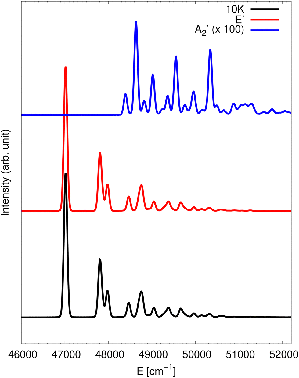 | ||
| Fig. 1 Photodetachment spectrum at 10 K (black trace). The partial contributions from the and the states are also shown in blue and red, respectively. The contribution is scaled by an arbitrary factor with respect to the one. | ||
Fig. 2 provides a simulation of the photodetachment spectrum at 435 K. Similarly to the 10 K spectrum, the full spectrum at 435 K is dominated by the partial spectra obtained via detachment into the state only. Therefore, the state contributions are not included in the presented spectra. When compared with the case at 10 K, the spectrum contains two additional lines below the assumed 0-0 line at 47 017 cm−1. These are hot bands corresponding to an initial NO3− state with one quantum in the anti-symmetric bending mode. From energy considerations, the line at 46313 cm−1 has to be the 401 line and the line at 46708 cm−1 is inferred to be 411 which is found 395 cm−1 above the 401 line. Again, the splittings of tunnelling multiplets of these final vibronic states are not resolved.
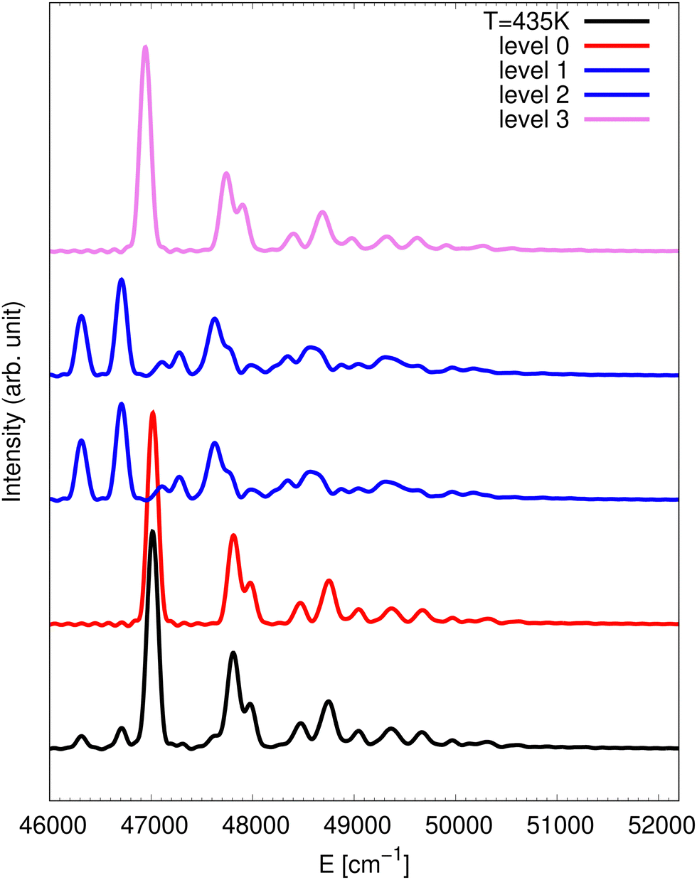 | ||
| Fig. 2 Theoretical spectrum at 435 K (black) corresponding to detachment to the 2E′ manifold. The contributions from the different vibrational states of the anion are also displayed: vibrational ground state in red, anti-symmetric bending in blue and umbrella in violet. | ||
An experimental photoelectron detachment spectrum covering the  , à 2E′′ and 2E′ energy range using a 6.424 eV photon energy was published in 2002.26 The recorded spectrum in the state energy range, from which an assumed linear baseline was subtracted, is presented in Fig. 3 and compared to the theoretical spectra at 10 K and 435 K. The only difference between the theoretical spectra of Fig. 3 and the ones in Fig. 1 and 2 is the resolution that is modeled here by a stronger damping of the autocorrelation functions. The optimal damping for which the theoretical spectra look similar to the experimental one is found to be at 50 fs. At this resolution, the vibrational structures seen in the higher resolution spectra collapse into a series of four very broad lines in very good agreement with the experimental spectrum. This sequence of peaks was interpreted as one vibrational progression with a 850 cm−1 frequency and was attributed in ref. 26 to an in-plane ν3 bending mode in reduced C2v symmetry. The current theoretical results, however, show that this is an oversimplified view since several vibronic levels contribute to each of the four experimental features. The low energy part of the experimental spectrum shows some intensity, which is reproduced in the 435 K spectrum (blue curve) but not present in the 10 K spectrum (black line). This means that the actual temperature of the experimental spectrum is sufficiently high to cause hot bands. The extraction of a temperature from comparison with the theory is not straigtht forward because the raw experimental spectrum26 contains overlapping signals from detachment to the 2E′ and to the à 2E′′ state. Therefore, the temperature was kept at 435 K in the simulation.
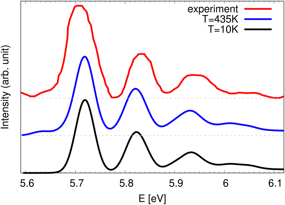 | ||
| Fig. 3 Comparison of low resolution theoretical spectra at 10 K (black) and 435 K (blue) corresponding to detachment to the 2E′ manifold with the experimental spectrum (red) from ref. 26. | ||
The shape of the photodetachment bands is a fairly indirect indicator of the nonadiabatic coupling strengths and the resulting nonadiabatic dynamics. However, the quantum dynamics simulations allow for a much more direct study of the coupling effects by studying the time-resolved population dynamics among the involved electronic states. The corresponding results are presented in the next section.
B. Nonadiabatic population dynamics
The time evolution of the adiabatic populations of the involved electronic states is computed for two different scenarios, after initial population of the à or the state manifold, respectively. In each case, the initial wave-packet is placed on a single diabatic component of the corresponding manifold, which, in the adiabatic picture, corresponds to a 1:1 population on the two adiabatic state components.37 The time evolution of the five adiabatic populations, Di, i = 0,…, 4, are presented in Fig. 4 for the à state (bottom panel) and for the state (top panel). The presented data correspond to a detachment into the x components of each doubly degenerate state. Identical curves are obtained for the detachment into the y components.
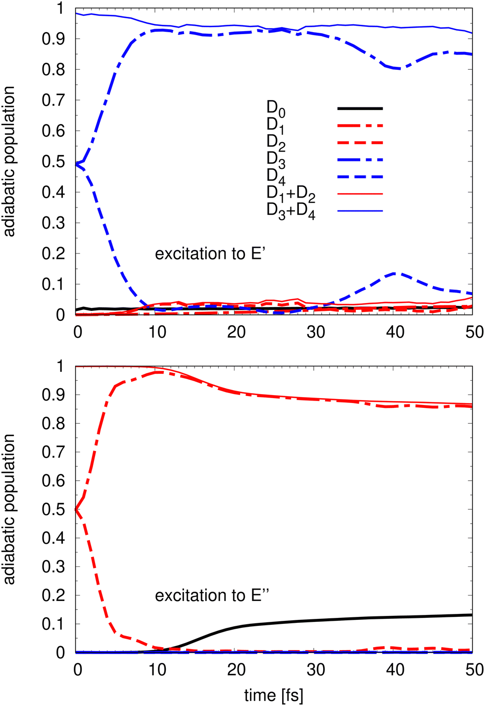 | ||
| Fig. 4 Evolution of the 5 adiabatic populations starting from an excitation to (top panel) and to à (bottom panel) for the first 50 fs. In addition to the five adiabatic populations Di, i = 0,4, the sum of the à and components are also presented. | ||
Upon detachment into the à state it takes only about 10 fs for the population to transfer almost completely from the upper D2 to the lower D1 adiabatic sheet of the E′′ state. This is followed by a small reduction of the D1 population compensated by the increase of population of the ground state D0. The D3 and D4 states do not get populated after detachment into the à state as can be expected given that the energy of the initial wave-packet is lower than the energy of these two upper adiabatic potentials. The ground state population is slowly increasing around 10 fs and after 50 fs, the population of the D0 ground state amounts to about 15%.
A very similar dynamics is observed when considering the detachment into the state. A very fast population transfer from the upper PES sheet of the 2E′ state component to the lower state component is followed by a slow population transfer to the lower à and state components. However, even the initial population shows a small contribution of a few % of the D0 ground state because the non-adiabatic couplings among the and the state are quite significant. The transfer out of the initially populated upper states, however, is slower compared to detachment into the à state and after 50 fs less than 10% of the population of the D3 + D4 manifold is transferred. A recurrence between the D3 and D4 (dashed and dot-dashed curves) is observed at 40 fs with a roughly 20% back transfer to the upper D4 state component. However, a complete back transfer to the initial 1:1 population ratio does never occur. This oscillation observed in the adiabatic population evolution is an indication of a relatively weak JT coupling in agreement with the PES model, which makes it more probable for the wave packet to populate the upper PES sheet due to a relatively small energetic separation.
For longer times, it is convenient to look at the sum of the D3 + D4 components and the sum of the D1 + D2 à components instead of the individual populations. Fig. 5 presents the evolution of such quantities up to 200 fs. Except for the very short time of 10–20 fs, the evolutions of the populations are very regular and nearly linear in time. 200 fs after the detachment into the state, 81% of the population is still in the D3 + D4 manifold and 14% has reached the D1 + D2 manifold while the population of the D0 ground stays about 5%. The transfer out of the D1 + D2 manifold after detachment into the à state is more efficient and after 200 fs, only 68% are still in the initial D1 + D2 manifold while 32% has transferred to the D0 ground state.
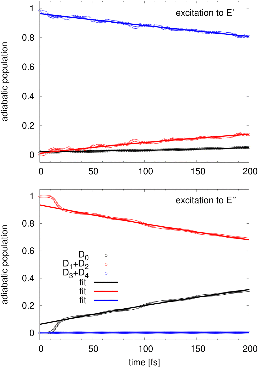 | ||
| Fig. 5 Adiabatic population evolution starting from an excitation to (top panel) and to à (bottom panel). Numerical populations (circles) are compared to the analytical model (lines). See text. | ||
The time evolution of the adiabatic populations indicates that the conical intersections other than at the D3h configurations are not relevant for the dynamics, which is in agreement with the interpretation of the simulated spectra. The rather linear time evolution curves together with the slow population transfer are an indicator of a simple statistical non-radiative decay. If this assumption is true, then the population dynamics should be reproducible by a simple kinetic model, which will be investigated next.
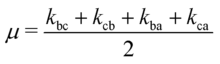
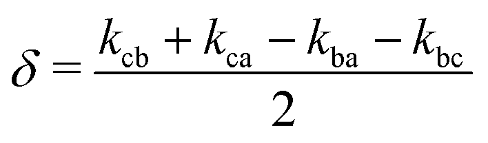
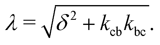
C. Kinetic model for non-radiative decay
In the following, the dynamics of the non-radiative decay is simulated like a reaction that can take different pathways. The initial population of the E′ state can decay directly to the à E′′ or the  state. The initial population of the à E′′ can transfer to the higher E′ state or decay directly to the
  state. Thus, the kinetic model with the corresponding rate coefficients is given by
 | (1a) |
 | (1b) |
Like in first order chemical reactions, the populations of the three states, [E′], [E′′] and  must satisfy
 | (2a) |
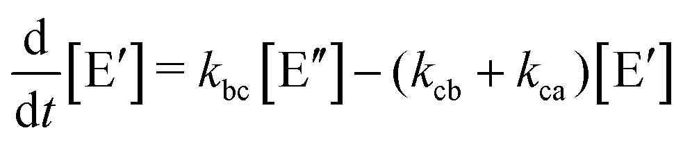 | (2b) |
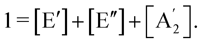 | (3) |
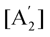 . The solution of these differential equations is given by
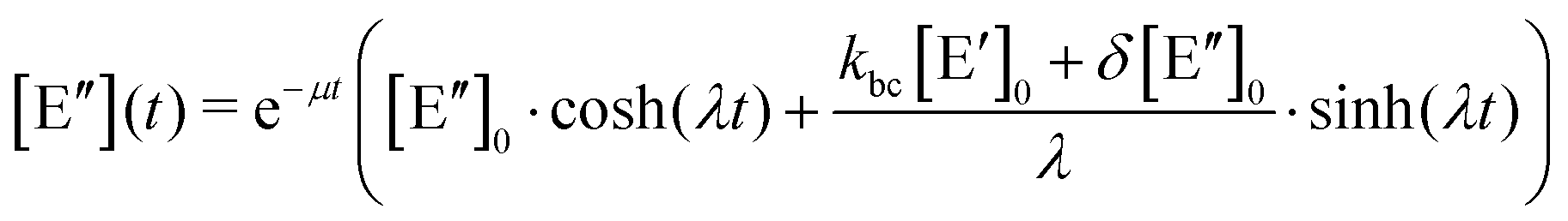 | (4a) |
 | (4b) |
 | (5a) |
 | (5b) |
 | (5c) |
| Rate constants [fs−1] | Full model | Simplified model |
|---|---|---|
| k ca | 3.25 × 10⁻⁵ | 0 |
| k cb | 8.79 × 10⁻⁴ | 8.78 × 10⁻⁴ |
| k bc | 6.42 × 10⁻⁶ | 0 |
| k ba | 1.58 × 10⁻³ | 1.58 × 10⁻³ |
Table 4 shows that the rate constant kba, which determines how rapidly the population transfers from the à to the ground state, has the largest value. This is coherent with the dynamics at long time as described above. The next largest value is kcb, which is close to half the value of kba (precisely it is 1.8 times smaller). The other two rate constants, kba and kca, are 50 and 250 smaller than kba. They seem sufficiently small to be neglected, which implies that the depopulation of the state goes via the à state and that the limiting step towards the ground state is the to à state step. Direct population transfer from the to the state seems to be negligible as is back transfer from the à to the state. To verify this hypothesis, a reduced model was fitted in which the transfer of populations is limited to the next state going down in energy, thus considering only kba and kcb. The results are basically indistinguishable from the full model on the scale of the figures.
The fact that the simple rate model reproduces the numerical adiabatic population time evolution that accurately is a clear indication that the conical intersections between the Ã, and states do not play a role here. The long-time population dynamics beyond the initial fast equilibration phase clearly is governed by statistical non-radiative decay due to weak nonadiabatic couplings and simple energy gap rules.
D. Discussion
While these results might seem rather unspectacular at first glance, they are in fact very enlightening for the understanding of nonadiabatic dynamics in general. It seems that over the past couple of decades it became kind of an unquestioned paradigm that the presence of a conical intersection always induces ultra-fast dynamics and non-radiative decay, which dominates the entire photochemistry. The present results show quite clearly that the presence of a conical intersection between two components of the à and states at low energy has basically no influence on the population dynamics. The reason in the present case is that the diabatic coupling is rather weak and of higher order. Thus, the dynamics becomes statistical just as if there was no conical intersection at all. It requires both a conical intersection and a strong diabatic coupling to induce the ultra-fast dynamics that is generally assumed to dominate the photochemistry. The present results show that both relevant and irrelevant conical intersections and thus non-statistical as well as statistical population dynamics are present in NO3. The ultra-fast decay takes place among the components of the JT active à and states due to the significant intra-state diabatic coupling among the components. After the wave packet is transferred to the lower sheet of each state manifold and equilibrated, the further dynamics becomes slow and statistical because the inter-state diabatic couplings are weak. Thus, the presence of a conical intersection might be a required but certainly not sufficient condition for ultra-fast radiative decay.
IV. Conclusions
A prediction of the NO3− photodetachment spectra at 10 K and 435 K in the energy range of the 2E′ NO3 state is proposed. The full quantum computation relies on an accurate diabatic model for the 5 lowest electronic surfaces of NO3, representing the  , 2E′′ (Ã) and 2E′ () states. The temperature effects are accounted for in a straightforward manner. Partial spectra using as initial condition several vibrational states of the anion are added to build the full spectrum taking into account the Boltzmann factors. Two parameters are not directly provided by the model and were determined previously by comparison with available experimental spectra at lower energies. These are the energy difference between NO3− and NO3 as well as the relative electron detachment cross-sections corresponding to the diabatic ground state and the diabatic 2E′ manifold. The predicted spectra at low and higher temperature hopefully will inspire new measurements. The band shape of the obtained spectrum indicates that the intra-state Jahn–Teller coupling is weaker in the 2E′ state than in the à 2E′′ state and that the inter-state pseudo Jahn–Teller non-adiabatic couplings as well as a low energy conical intersection between the à and manifold play little role.
The conclusions drawn from the analysis of the computed spectra may be checked experimentally but they are rather indirect. However, the accurate quantum dynamics simulations also allow for a direct study of the effects leading to the above interpretation of the spectra. This is achieved by the analysis of the adiabatic population dynamics among the three state manifolds. It is found that during a very short equilibration time of 10 fs, the population localises on the lower sheet of the Jahn–Teller coupled D1, D2 and of the D3, D4 state manifolds, respectively. This is a direct consequence of the Jahn–Teller symmetry-induced conical intersections at the D3h geometries as is well established. The weaker Jahn–Teller coupling within the (D3/D4) state manifold is manifested by a slightly slower non-radiative decay and also a recurrence (back transfer) into the D4 component. Such a recurrence is absent among the à (D1/D2) components supporting the difference in coupling strength, which is also in agreement with the analytical diabatic potential model. After this initial equilibration period of roughly 10 fs, which is dominated by the conical intersections at D3h configurations and the corresponding Jahn–Teller effect, a much slower inter-state non-radiative decay is observed. Despite the presence of the low energy conical intersection between the D2 and D3 PES sheets, the wavepackets are not strongly affected by this additional conical intersection. It turns out that the inter-state couplings are too weak to induce strong non-adiabatic effects and thus the population dynamics at longer times becomes slow and statistical. This interpretation is supported further by a kinetic model for the population dynamics, which reproduces the quantum dynamics results almost perfectly for times longer than 10 fs. The kinetics model also supports a cascading mechanism for the non-radiative decay after populating the state. The population decays from the state to the à state and from the à state to the state while direct decay from to or back transfer is completely negligible. Furthermore, decay from to à is slower than from à to despite the Ö conical intersection. This demonstrates that the paradigm that photochemistry is dominated by conical intersections and that conical intersections (“always”) induce ultra-fast dynamics should be taken with caution.
Conflicts of interest
There are no conflicts of interest to declare.Acknowledgements
Part of this work was generously supported by the Deutsche Forschungsgemeinschaft (DFG). AV was partially supported by the CNRS and by the University of Rennes 1 via the IRN MCTDH. AV and WE are indebted to Wolfgang E. Ernst for valuable discussions about in particular Jahn–Teller effects and their importance in various fields.38References
- M. Mayer, L. S. Cederbaum and H. Köppel, J. Chem. Phys., 1994, 100, 899 CrossRef CAS.
- M. Okumura, J. F. Stanton, A. Deev and J. Sommar, Phys. Script., 2006, 73, C64 CrossRef CAS.
- J. F. Stanton, J. Chem. Phys., 2007, 126, 134309 CrossRef PubMed.
- S. Mahapatra, W. Eisfeld and H. Köppel, Chem. Phys. Lett., 2007, 441, 7 CrossRef CAS.
- S. Faraji, H. Köppel, W. Eisfeld and S. Mahapatra, Chem. Phys., 2008, 347, 110 CrossRef CAS.
- J. F. Stanton, Mol. Phys., 2009, 107, 1059 CrossRef CAS.
- J. F. Stanton and M. Okumura, Phys. Chem. Chem. Phys., 2009, 11, 4742 RSC.
- C. S. Simmons, T. Ichino and J. F. Stanton, J. Phys. Chem. Lett., 2012, 3, 1946 CrossRef CAS.
- Z. Homayoon and J. M. Bowman, J. Chem. Phys., 2014, 141, 161104 CrossRef PubMed.
- W. Eisfeld, O. Vieuxmaire and A. Viel, J. Chem. Phys., 2014, 140, 224109 CrossRef PubMed.
- W. Eisfeld and A. Viel, J. Chem. Phys., 2017, 146, 034303 CrossRef PubMed.
- A. Viel and W. Eisfeld, Chem. Phys., 2018, 509, 81 CrossRef CAS.
- A. Viel, D. M. G. Williams and W. Eisfeld, J. Chem. Phys., 2021, 154, 084302 CrossRef CAS PubMed.
- W. Eisfeld and K. Morokuma, J. Chem. Phys., 2000, 113, 5587 CrossRef CAS.
- W. Eisfeld and K. Morokuma, J. Chem. Phys., 2001, 114, 9430 CrossRef CAS.
- A. Viel and W. Eisfeld, J. Chem. Phys., 2004, 120, 4603 CrossRef CAS PubMed.
- W. Eisfeld and A. Viel, J. Chem. Phys., 2005, 122, 204317 CrossRef PubMed.
- D. M. G. Williams and W. Eisfeld, J. Chem. Phys., 2018, 149, 204106 CrossRef PubMed.
- T. Lenzen, W. Eisfeld and U. Manthe, J. Chem. Phys., 2019, 150, 244115 CrossRef PubMed.
- D. M. G. Williams, A. Viel and W. Eisfeld, J. Chem. Phys., 2019, 151, 164118 CrossRef PubMed.
- D. M. G. Williams and W. Eisfeld, J. Phys. Chem. A, 2020, 124, 7608 CrossRef CAS PubMed.
- G. Sprenger, Z. Elektrochem., 1931, 37, 674 CAS.
- E. J. Jones and O. R. Wulf, J. Chem. Phys., 1937, 5, 873 CrossRef CAS.
- A. Weaver, D. W. Arnold, S. E. Bradforth and D. M. Neumark, J. Chem. Phys., 1991, 94, 1740 CrossRef CAS.
- M. C. Babin, J. A. DeVine, M. DeWitt, J. F. Stanton and D. M. Neumark, J. Phys. Chem. Lett., 2020, 11, 395 CrossRef CAS PubMed.
- X.-B. Wang, X. Yang, L.-S. Wang and J. B. Nicholas, J. Chem. Phys., 2002, 116, 561 CrossRef CAS.
- D. A. Hrovat, G.-L. Hou, B. Chen, X.-B. Wang and W. T. Borden, Chem. Sci., 2016, 7, 1142 RSC.
- I. Seidu, P. Goel, X.-G. Wang, B. Chen, Z.-B. Wang and T. Zeng, Phys. Chem. Chem. Phys., 2019, 21, 8679 RSC.
- S. Dobrin, B. Boo, L. Alconcel and R. Continetti, J. Phys. Chem., 2000, 104, 10695 CrossRef CAS.
- H. D. Meyer, U. Manthe and L. S. Cederbaum, Chem. Phys. Lett., 1990, 165, 73 CrossRef CAS.
- U. Manthe, H. D. Meyer and L. S. Cederbaum, J. Chem. Phys., 1992, 97, 3199 CrossRef CAS.
- U. Manthe, J. Chem. Phys., 2008, 128, 064108 CrossRef PubMed.
- U. Manthe, J. Chem. Phys., 1996, 105, 6989 CrossRef CAS.
- A. Viel, W. Eisfeld, S. Neumann, W. Domcke and U. Manthe, J. Chem. Phys., 2006, 124, 214306 CrossRef PubMed.
- C. Evenhuis, G. Nyman and U. Manthe, J. Chem. Phys., 2007, 127, 144302 CrossRef PubMed.
- T. Weike, D. M. G. Williams, A. Viel and W. Eisfeld, J. Chem. Phys., 2019, 151, 074302 CrossRef PubMed.
- The adiabatic population of the two state components is exactly 1:1 for an isolated doubly degenerate state. The 2E′ state has an additional coupling to the ground state by a significant pseudo Jahn–Teller coupling and thus a small part of the adiabatic population is found in the ground state.
- W. E. Ernst and H. Köppel, Chem. Phys., 2015, 460, 1 CrossRef CAS.
| This journal is © the Owner Societies 2022 |