Dynamics and outcomes of binary collisions of equi-diameter picolitre droplets with identical viscosities

Abstract

The dynamics of binary collisions of equi-diameter picolitre droplets with identical viscosities, varying impact speeds and impact angles have been investigated experimentally and compared to collision outcome prediction models. Collisions between pairs of pure water droplets with a viscosity of 0.89 mPa s and pairs of aqueous-sucrose (40% w/w) droplets with a viscosity of 5.17 mPa s were examined. The colliding droplets were ∼38 μm in diameter, which is around ten times smaller than those previously investigated when examining the effect of viscosity on the outcome of binary droplet collisions. Varying the impact speed and angle resulted in different collision outcomes, including coalescence, reflexive separation and stretching separation. The collision outcomes were plotted on two viscosity dependent regime maps. The regime boundaries are generally in agreement with earlier literature for both high and low viscosity cases. The agreement between experiment and theory, for both fluids, gives more confidence in the models tested here to predict collision outcomes for droplets of this size and these viscosities.

---

1 Introduction

The outcome of binary aerosol droplet collisions has relevance to many academic and industrial fields of research including atmospheric science, combustion engines and spray drying.^1–3 The outcomes of droplet collisions influence the aerosol size distributions as collisions alter both the average droplet size and the overall number concentration. Predicting and characterising evolving size distributions is important, for example, in the case of inhaled drug formulations produced by spray drying,⁴ where the uniformity affects the dose delivered to the patient and the drug efficacy.⁵ Previous research has exploited the dynamics of binary droplet collision and coalescence events to resolve a variety of physical properties and dynamic processes. For example, the controlled coalescence of neighbouring droplets trapped in a dual optical tweezers arrangement has been applied to measure the surface tension and viscosity for highly viscous microscopic droplets.^6–8 High-resolution imaging of colliding droplet streams has been employed to probe the collision dynamics of miscible droplets⁹ and combined with Raman spectroscopy^10,11 and separately, mass spectroscopy,¹² to probe rapid reaction rates. Reaction dynamics have been probed further firstly using fluorescence microscopy,¹³ and subsequently by combining a branched quadrupole with fluorescence spectroscopy and single droplet paper spray mass spectrometry, to initiate reactions through controlled binary droplet collisions and analyse the temporal evolution of the reaction products.¹⁴

In addition to research utilizing droplet collisions to probe droplet dynamics, the characterisation of outcomes of binary collisions using a high-resolution imaging technique has been extensively studied.¹⁵ ‘Outcome’ is defined as the state of the liquid matter after the collision process is complete. These outcomes are: (i) bouncing, where the droplets meet and reflect away from each other after impact; (ii) slow coalescence, where the droplets coalesce without significant deformation and the interaction time is sufficiently long for the interfaces to merge by diffusion; (iii) fast coalescence, where the droplets coalesce with significant deformation and the interfaces break and merge; (iv) stretching separation, where the droplets graze past each other and temporarily coalesce via a ligament, but then separate into two or more droplets; and (v) reflexive separation, where the droplets impact roughly head-on and temporarily coalesce as their interfaces ‘pancake’, but then pass through each other due to high inertia, separating into two or more droplets. Studies of the outcomes of binary droplet collisions have largely focused on droplets of a microlitre volume. While studies of droplets of this size have evolved to investigate more sophisticated systems, such as ternary collisions¹⁶ and non-Newtonian fluids,¹⁷ few studies have experimentally investigated the outcomes of collisions of picolitre droplets. Brenn and Kolobaric investigated collisions of droplets as small as 60 μm in diameter, however their analysis focused on the formation of satellite droplets and the fast coalescence/stretching separation boundary.¹⁸

The aim of the present investigation is to compare the measured outcomes of binary collisions of picolitre droplets observed with microsecond time-resolution with models of the coalescence/stretching separation and coalescence/reflexive separation boundaries. These boundaries have previously been verified for droplets an order of magnitude larger in size with measurement time-resolutions of typically 0.1–1 ms. In addition to pure water, a viscous 40% aqueous-sucrose solution is investigated in order to probe the well documented shift in the coalescence/reflexive separation boundary, due to viscous effects, observed in collisions of larger droplets.^19–23

Binary droplet collisions can be characterised by non-dimensional parameters, based on the liquid droplet properties, and their values can be used to infer the likely outcome of a collision event. We adopt the same terminology as Al-Dirawi and Bayly²⁴ here. The first dimensionless parameter is the Weber number We, which describes the ratio between the inertial and cohesive forces, and is calculated from the density ρ, surface tension σ, diameter d and magnitude of the relative velocity of the two droplets u_rel (see Fig. 1). In the case of droplets of unequal size, the diameter of the smaller droplet is used to calculate the Weber number. Here, we report measurements for identically sized droplets, d₁ = d₂, and the droplet size ratio

Fig. 1 A schematic of the geometry of binary droplet collisions, showing two points in time. Prior to collision, the droplets begin in positions 1 and 2, and move with velocities u₁ and u₂, respectively. Positions 1′ and 2′ represent the moment of collision of the droplets, with b indicating the projected separation distance between the centre of one droplet (the droplet in position 1′) normal to the relative velocity, u_rel plotted from the centre of the other droplet (the droplet in position 2′). The enclosed angle, θ, between the relative velocity vector and the distance between the centre of the two colliding droplets is 0° for a head-on collision and 90° for a grazing collision.

The second dimensionless number to characterise the collision is the impact parameter B, which describes the impact geometry and is defined as,

where b is the projected separation distance between the centre of one droplet normal to the relative velocity plotted from the centre of the other droplet (see Fig. 1). The Ohnesorge number Oh, characterises the relative importance of viscosity μ compared to the combined effect of inertial and surface tension forces on the collision outcome:

In the case of droplets of unequal size, the diameter of the smaller droplet is used to calculate the Ohnesorge number. Oh ∼ 0.12 indicates the threshold between the viscosity and surface tension dominated collision regimes.²³

Krishnan and Loth provide a comprehensive review of the regime maps, B = f(We), that can be used to assess the likely outcomes of identical binary droplet collisions.¹⁵ Various models for the fast coalescence/stretching separation boundary have been suggested. We consider two models for this boundary: Ashgriz and Poo²⁵ whose model considers only the impact parameter and droplet size ratio, and Jiang et al.²¹ with an adaptation from Sommerfeld and Pasternack,²⁶ whose models take viscous losses into account by including the Ohnesorge number. Ashgriz and Poo²⁵ also suggested a model for predicting the fast coalescence/reflexive separation boundary, which again neglected viscous losses. In order to account for the effect of droplet viscosity on droplet collision outcomes, this model has been offset towards higher We using Oh correlations to determine the critical Weber number at B = 0. A number of Oh correlations have been suggested. Here, we consider the Qian and Law²⁰ correlation, previously shown to give a good approximation up to Oh = 0.1.

This work will evaluate the appropriateness of existing models for predicting collision outcomes of droplets (∼38 μm diameter) approximately one tenth of the size of the smallest droplets studied previously. Two fluids of low and high viscosity are chosen to examine the consistency between the models and measurements in the upshift in boundary between coalescence and reflexive separation anticipated from the work of Al-Dirawi and Bayly.²⁴ Both slow coalescence and bouncing outcomes are not observed in our experimental data as they only arise at low Weber number.^24,26 Section 2 will describe the experimental methodology including details of the image analysis used to calculate We and B. Section 3 will describe the results of the study, split into 3 sections: Section 3.1 will report images of observed collision outcomes, Section 3.2 will compare the visual similarity of collisions of the same outcome with extreme placements on the regime map and Section 3.3 will compare the measured outcomes from this study with existing models.

2 Experimental methodology

2.1 The experimental setup

We present studies of the collision of pairs of picolitre (∼38 ± 1 μm) droplets of the same composition, considering two liquids with different viscosities to test the appropriateness of different treatments for predicting the collision outcomes. Specifically, we look at the collision of droplets of pure water with a viscosity of 0.89 mPa s and droplets of an aqueous-sucrose solution (40% w/w) shown by Telis et al. to have a viscosity of 5.17 mPa s at 25 °C.²⁷ All measurements presented here were performed under typical conditions (∼50% RH, measured laboratory temperature 25 ± 1 °C) Table 1.

Table 1 Physical properties of the 2 liquids used in this work at 25 °C. Literature values are given for density (ρ), surface tension (σ) and viscosity (μ). Ohnesorge values (Oh) were calculated using eqn (3) for 38 μm diameter droplets

Liquid	ρ (kg m^−3)	σ (mN m^−1)	μ (mPa s)	Oh
Water	997.0	72.0	0.89	0.017
Sucrose 40% (w/w)	1176.5	74.1	5.17	0.090

---

The droplet collision events were instigated by targeting two frequency-synchronised streams of uniform droplets, generated by piezo-electric droplet-on-demand dispensers, such that their trajectories intersected. The streams were manoeuvred to ensure droplets from both streams reached the intersection point at coincident times, creating a continuous sequence of uniform collisions, shown schematically in Fig. 2.

Fig. 2 A schematic of the experimental set-up showing the droplet dispensers and imaging assembly used to create and study the droplet collisions, respectively.

The droplet streams were created using piezo-driven droplet-on-demand (DoD) dispensers (MicroFab, 30 μm orifice diameter) driven with a 10 Hz series of regular, uniform voltage pulses. The pulse profile (i.e. width and amplitude), which influences the initial size and velocity of the droplets produced, was defined using bespoke software and generated by an arbitrary function generator (Keysight, Trueform 33500B Series). The dispensers were both individually mounted on opposing xyz translation/360° rotation stages (Thorlabs) allowing the absolute position and dispensing angle to be manually controlled, as shown in Fig. 2. The dispenser tips were separated by ∼20 mm, with dispensing angles just below the horizontal. This prevented the droplet stream from one dispenser striking the tip of the other dispenser (and impeding the droplet generation). The generation of uniform droplets at well-defined time points allowed the collision event to be reproduced reliably at 10 Hz, and a complete time-sequence of a collision geometry could then be acquired. Given the high initial droplet velocities and relatively close proximity of the dispensers, the collisions were calculated to occur within the first millisecond of the droplet lifetimes. This provided enough time for the droplet morphologies to relax to spheres prior to collision but insufficient time for any significant evaporation to occur that would lead to a change in composition.

Stroboscopic imaging was used to observe the outcome of collision events with very high temporal (0.25 ns) and spatial (∼1 μm) resolution. The stroboscopic illumination assembly consisted of a white LED, strobed at the same frequency as the droplet generation with a 500 ns pulse. Stroboscopically illuminated images were collected using a microscope objective (Optem, M Plan APO, 0.42 NA, 20× Mag), expanded using a zoom assembly (Navitar, 4× Mag) and captured with the CCD camera (Jai, GO-2400M-USB). The image acquisition (i.e. LED pulse and image capture) was triggered using the DoD dispenser pulse following the incorporation of a variable delay (Quantum Composers, 9520 Series Pulse Generator, 0.25 ns delay resolution), with one image collected per dispenser pulse. At a constant time delay, each image captured the same moment during the approach, collision or post-collision sequence. Varying the dispenser/image acquisition delay between acquired images allowed the progress of the collision to be monitored with a temporal resolution limited only by the resolution of the delay generator (0.25 ns), although a temporal resolution of ∼1 μs was more typically used. This approach means each sequential image contains a subsequent pair of droplets, which clearly demonstrates the reproducibility of the droplet-on-demand generation technique.

The experimental setup allowed simple adjustment to both B and We between experiments. B was adjusted by changing the trajectory of one droplet stream relative to the other, by, for example, slightly rotating one of the dispensers. The method allowed the full range of impact geometries to be accessed between head-on (i.e. B ∼ 0) and barely grazing (B ∼ 1) collisions. We was adjusted by manipulating the DoD dispenser pulse voltages and, hence, the relative velocities of the colliding droplets. This allowed We to be varied between ∼10 and ∼150.

2.2 Image processing and analysis

The pre-collision droplet velocities, sizes and impact angles were directly calculated from the stroboscopic images using custom-written software. The procedure for isolating the droplets from an image and extracting the relevant physical information is shown schematically in Fig. 3. Firstly, the raw image was binarised against a user-selected pixel intensity threshold to identify and isolate the droplet outlines/boundaries from the background. Secondly, the droplet diameters were calculated from the height or width of the relevant bounding shape (typically a circle for a spherical droplet) and the shape centres used to identify the relative locations of the droplets within the main image. Finally, the pre-collision droplet trajectories, determined from the change in droplet location between 2 images separated by a given change in the delay time (typically 15 μs), allowed the individual velocities, relative velocity and impact angle to be calculated. The field-of-view of the image was calibrated prior to each experiment using a micrometre graticule, allowing length scales to be converted from pixels to micrometres.

Fig. 3 The image processing used to calculate droplet velocities and impact angle. The bottom image shows the trajectories of the droplets at the moment prior to collision.

Although a droplet stream produced by a DoD dispenser is highly uniform, small variations do exist in trajectories of different droplets within the stream. This artifact led to small, but not insignificant variations in recorded We and B, depending on which pre-collision images, or frames, were used in the calculation of the relative velocity and impact angle (remembering that each frame contained a unique set of droplets). To quantify the magnitude of this uncertainty in each binary droplet collision experiment, the relative velocity and impact angle were recalculated using ∼20 different pairs of pre-collision frames (with each pair maintaining a 15 μs temporal separation). Following removal of extreme outliers in the retrieved data, corresponding to occasional jitters in the droplet stream, the mean and standard deviation in velocity and impact angle, and by propagation, in We and B were calculated for each collision experiment. This variation was considered to represent the largest uncertainty in the measurements presented here and correspond to the error bars in We and B in the data sets presented below.

3 Results and discussion

3.1 Identifying collision outcomes

We compare sequences of images collected from collision events of pure water and aqueous sucrose solution droplets in Fig. 4. By varying B and We, the outcome of the collision can be changed from coalescence to reflexive or stretching separation. The evolution of any one collision falls into one of these three discrete outcomes, and can be attributed to the appropriate category from post-coalescence images. An exception to this is discussed in Section 3.3, where a ‘mixed outcome’ can occasionally be observed following collisions of aqueous-sucrose droplets. This is a consequence of the stroboscopic imaging technique and the instability in dispensing viscous solution droplets, leading to a reduction in reproducibility of the observed collision outcome. The timestep between images in the sequences in Fig. 4 are not uniform, rather frames have been chosen to highlight the evolution of the various outcomes. Note how the Weber number is the same for all three water examples shown, highlighting that all three outcomes are accessible simply by varying the impact parameter for droplets of identical composition at a particular relative velocity.

Fig. 4 Examples of the (a) coalescence (b) reflexive separation and (c) stretching separation collision outcomes accessed during this study for (i) water and (ii) sucrose.

3.2 Similarities in collision dynamics across the We–B regime map

Collision outcome models can be used to identify the boundaries for different outcomes in the We–B regime map. Shown schematically, shaded regions in Fig. 5 outline the predicted outcome regions estimated from the models of Ashgriz & Poo and Qian & Law for the coalescence/stretching separation and coalescence/reflexive separation boundaries, respectively. The models predict that collisions of quite different values of We and B can result in the same collision outcome, and this is what is also observed in experimental data. For example, collisions of pairs of droplets with We = 20 and B = 1 or with We = 150 and B = 0.3 should both yield a stretching separation outcome.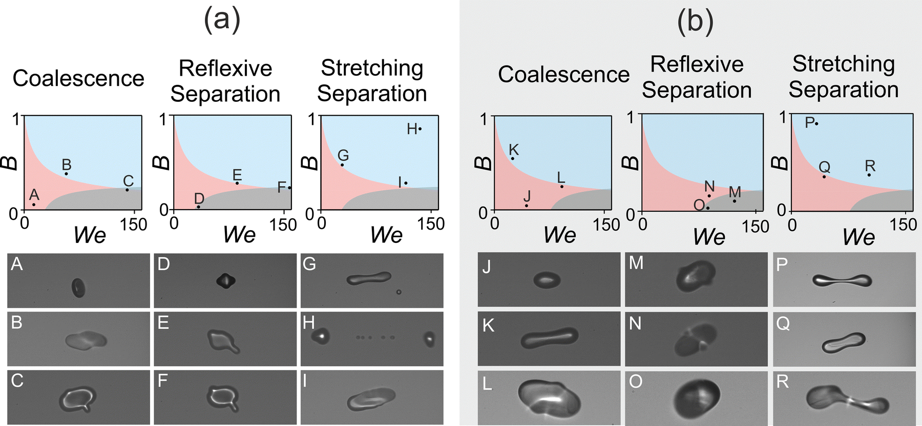

Fig. 5 A comparison of the same outcome at different points on the regime map for (a) water and (b) sucrose. The shaded pink, blue and grey regions correspond to the expected coalescence, stretching separation and reflexive separation regions, respectively. These regions were determined using Ashgriz and Poo's model for the coalescence/stretching separation boundary and Qian and Law's model for the coalescence/reflexive separation boundary. The images shown were captured 20 μs after the initial point of collision.

Fig. 5 compares the evolution of droplet collisions at extreme points within each outcome region of the regime map, showing images 20 μs after the initial point of collision. Images captured after this time were occasionally out of focus due to trajectories that took droplets out of the narrow depth of field. While the overall outcome of the collision was obvious regardless of the clarity of the focus, images captured at 20 μs were chosen for this comparison in order to compare the visual similarity of the collision outcomes.

For coalescence and reflexive separation, Fig. 5a (water droplets), similarities are clear in the evolution of collisions after 20 μs at quite extreme points within each region. This is perhaps unsurprising, given events A, B and C are found nearby on the regime map to D, E and F, respectively. The precise angle and speed of the collision determines its further evolution after the instant shown here. Due to the wide extent of the We–B parameter space for the stretching separation region, more widely spread events, G, H and I, can be compared than for the smaller coalescence and reflexive separation regions. The images of stretching separation in Fig. 5a (water droplets) appear to vary significantly, both amongst themselves and compared to the other two outcomes. At this point in time, droplets in H have already collided and separated, whereas all other images show the collision prior to relaxation (coalescence) or separation (reflexive or stretching separation) of the droplet(s). It should be noted that the precise moment the outcome can be said to be ‘complete’ does vary although the outcome reaches completion faster for higher Weber numbers, i.e. at higher impact velocities. This is likely due to the increased inertia of these droplets.

For images in Fig. 5b (aqueous sucrose droplets), there is no significant variation in the visual development of the outcome with varying We and B at 20 μs for each outcome. This could, perhaps, be due to the viscous effects of this fluid on the evolution of collisions of these droplets. Although relatively high Weber numbers were accessed (>100), the viscosity of the fluid appears to slow the completion of the collision, resulting in visually similar images at 20 μs.

3.3 Comparison of observed outcomes with existing models

In total, we explored the collision outcomes from 147 pairs and 126 pairs of impact parameter and Weber number for pure water and an aqueous-sucrose solution, respectively. The regime maps of binary collisions of 38 ± 1 μm diameter droplets of pure water and 40% w/w aqueous-sucrose solution are shown in Fig. 6. Despite the droplets used in this study being an order of magnitude smaller than previous studies, the collision boundaries are broadly consistent with the expected regimes. For collisions of water droplets, the experimental results for stretching separation and reflexive separation are generally confined to their expected regions. The results for coalescence span a larger region than predicted, with unexpected coalescence outcomes occurring at We > 100. For collisions of aqueous-sucrose droplets, all three outcomes are confined to their expected regions. The large number of collisions examined at a We ∼ 30 is a consequence of limitations with stable operation of the droplet dispenser. When using a solution of such viscosity, only a narrow selection of voltage pulses successfully ejects a droplet. The voltage used directly correlates to the velocity, and therefore the Weber number of the droplets. Despite this limitation, sufficient data was acquired across the We–B parameter space to compare this experimental data to existing models. Occasionally, the same measured impact speed and angle resulted in different outcomes (e.g.Fig. 6b, We ∼ 45, B = 0.35, coalescence (red triangle) and stretching separation (blue square)). Since, generally, the data fit the expected outcome regions and these occurrences appear near the boundaries, it is likely there is a marginal error in the determination of the impact speed and/or angle, resulting in small mispositions of the data.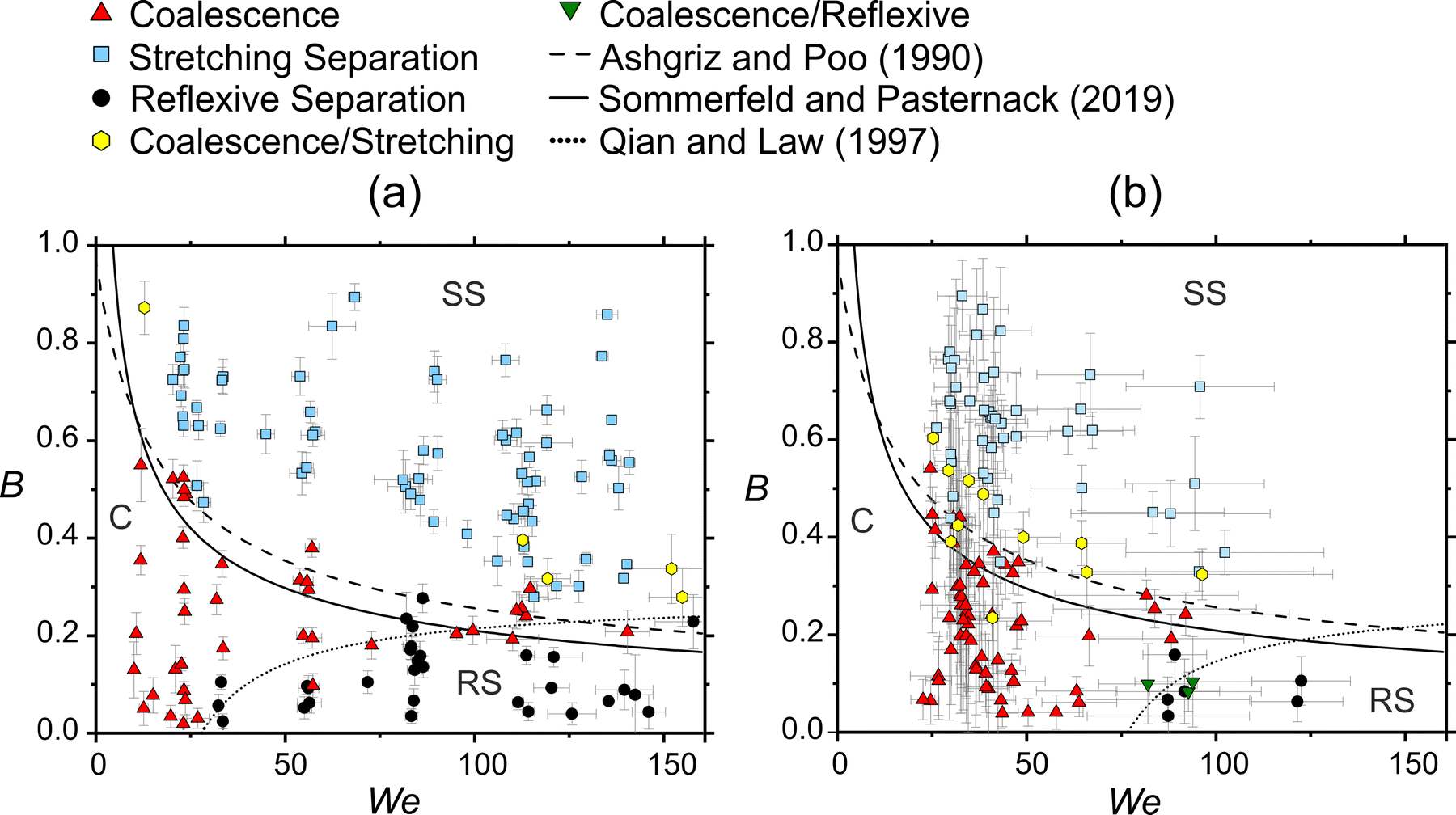

Fig. 6 Regime maps of binary droplet collisions: (a) water (Oh = 0.017) and (b) sucrose (Oh = 0.090). Error bars are standard deviation of the mean. C, SS and RS denote the outcome regions; coalescence, stretching separation and reflexive separation, respectively.

Ashgriz and Poo's parameterisation for the coalescence/stretching separation boundary appears to be more consistent with the measured boundary than the model of Sommerfeld and Pasternack, both for collisions of pure water droplets and for aqueous-sucrose solution droplets. Unlike Ashgriz and Poo, Sommerfeld and Pasternack's model incorporates a size dependence. Given the uncertainties associated with the impact parameter and Weber number for water droplet collisions, the accuracy of the marginal shift of the boundary arising from the dependence on particle size for the coalescence/stretching separation boundary cannot be assessed in our measurements. Similarly, for aqueous sucrose droplet collisions, the opportunity to resolve the more significant shift in the boundary is compromised by the greater instability in droplet generation which leads to larger uncertainties in impact parameter and Weber number. Qian and Law's model for the coalescence/reflexive separation boundary represents the measured collision outcomes of both water and aqueous sucrose droplets with high fidelity. It is clear that changes to the viscous properties of the droplets have a more pronounced effect on the position of the boundary of reflexive than stretching separation. This is reflected in the inclusion of the Ohnesorge number, which is a size-dependent parameter (eqn (3)), in Qian and Law's model for the reflexive separation boundary.

Due to the use of a stroboscopic imaging technique, each frame of a particular outcome video is comprised of different pairs of droplets. Occasionally, this would result in the observation of an apparent ‘mixed outcome’ in which sequential frames apparently showed alternating collision outcomes. Mixed outcomes occurred close to the outcome boundaries, suggesting that the use of reproducible droplet-on-demand dispensers with a stroboscopic technique can lead to small variations in the droplet speed and/or impact angle between frames. Mixed coalescence/stretching separation outcomes and coalescence/reflexive separation outcomes are shown in the data in Fig. 6 as yellow hexagons and green triangles, respectively. Mixed outcomes were more frequently observed in collisions of sucrose droplets, which is likely due to the reduced reproducibility of these droplets. The sucrose droplets require a high voltage pulse (>60 V) in order to dispense due to their higher viscosity, which is close to the limit of capacity for the dispensers, and lead to greater variations in the speed and angle of the droplets produced. These variations also account for the large error bars in the sucrose data, seen in Fig. 6b. An alternative high-speed imaging method could be adopted in order to capture the same pair of droplets through time. However, in order to achieve the same time resolution as the stroboscopic technique (Δt = 15 μs) described here, a sampling rate of >65 000 frames per second is required. High frame rate cameras are capable of such sampling rates; however, these instruments are expensive, therefore the benefit of observing the same pair of droplets through time would need to be considered against this cost.

4 Conclusion

Sequences of images were collected from collision events of picolitre pure water and aqueous-sucrose solution droplets, the outcome of each event was easily determined. Two regime maps, novel due to the small droplet size, were developed and shown to be broadly consistent with previous studies of droplets ∼10 times larger. The model for the coalescence/stretching separation boundary developed by Ashgriz and Poo was shown to be appropriate for predicting the outcome of collisions of this size. This model is size-independent, indicating that perhaps the minimal size dependence of this boundary is beyond the resolution of the technique used in this work. This model also has little dependence on the viscous properties of the solution, therefore this boundary remained largely unchanged between the pure water and aqueous-sucrose solution. The coalescence/reflexive separation boundary, however, is shown to be highly dependent on the viscosity of the droplets. A clear shift in this boundary to higher Weber number is observed when the regime maps of the two solutions are compared. This shift is reflected in Qian and Law's model for the boundary, which takes viscous properties and droplet size into account by including the Ohnesorge number. Overall, the experimental data show a general agreement with the models tested here, indicating that droplet size has no significant effect on the outcome regions of the regime map. The coalescence/reflexive separation boundary appears to be well defined by Qian and Law's viscous and size-dependent model, however a more rigorous size-dependent model for the coalescence/stretching separation boundary could be explored. A comparison of collisions at extreme points within each outcome region does not show significant visual differences. However, the time taken for the outcome to be complete appears to be dependent on the Weber number.

Author contributions

Lauren P. McCarthy: software, data curation, formal analysis, visualisation, writing – original draft preparation, Peter Knapp: methodology, investigation, software, formal analysis, writing – original draft preparation, visualisation, Jim S. Walker: methodology, software, writing – review and editing, Justice Archer: investigation, Rachael E. H. Miles: conceptualization, investigation, Marc E. J. Stettler: supervision, writing – review and editing, Jonathan P. Reid: supervision, writing – review and editing.

Conflicts of interest

There are no conflicts to declare.

Acknowledgements

The authors acknowledge funding from the Engineering and Physical Sciences Research Council (EPSRC, EP/N025245/1). L. P. M. and P. K. acknowledge funding from EPSRC (EP/S023593/1).

References

1. U. K. Krieger, C. Marcolli and J. P. Reid, Chem. Soc. Rev., 2012, 41, 6631–6662.
2. S. L. Post and J. Abraham, Int. J. Multiphase Flow, 2002, 28, 997–1019.
3. C. Sadek, P. Schuck, Y. Fallourd, N. Pradeau, C. Le Floch-Fouéré and R. Jeantet, Dairy Sci. Technol., 2014, 95, 771–794.
4. W. Yang, J. I. Peters and R. O. Williams 3rd, Int. J. Pharm., 2008, 356, 239–247.
5. G. Pilcer and K. Amighi, Int. J. Pharm., 2010, 392, 1–19.
6. B. R. Bzdek, J. P. Reid, J. Malila and N. L. Prisle, Proc. Natl. Acad. Sci. U. S. A., 2020, 117, 8335–8343.
7. B. R. Bzdek, R. M. Power, S. H. Simpson, J. P. Reid and C. P. Royall, Chem. Sci., 2016, 7, 274–285.
8. R. M. Power, S. H. Simpson, J. P. Reid and A. J. Hudson, Chem. Sci., 2013, 4, 2597–2604.
9. J. Kohno, M. Kobayashi and T. Suzuki, Chem. Phys. Lett., 2013, 578, 15–20.
10. T. Suzuki and J. Kohno, J. Phys. Chem. B, 2014, 118, 5781–5786.
11. K. Anahara and J. Kohno, J. Phys. Chem. B, 2017, 121, 9895–9901.
12. J. K. Lee, S. Kim, H. G. Nam and R. N. Zare, Proc. Natl. Acad. Sci. U. S. A., 2015, 112, 3898–3903.
13. R. D. Davis, M. I. Jacobs, F. A. Houle and K. R. Wilson, Anal. Chem., 2017, 89, 12494–12501.
14. M. I. Jacobs, J. F. Davies, L. Lee, R. D. Davis, F. Houle and K. R. Wilson, Anal. Chem., 2017, 89, 12511–12519.
15. K. G. Krishnan and E. Loth, Int. J. Multiphase Flow, 2015, 77, 171–186.
16. H. Hinterbichler, C. Planchette and G. Brenn, Exp. Fluids, 2015, 56, 190.
17. G. Finotello, S. De, J. C. R. Vrouwenvelder, J. T. Padding, K. A. Buist, A. Jongsma, F. Innings and J. A. M. Kuipers, Exp. Fluids, 2018, 59, 113.
18. G. Brenn and V. Kolobaric, Phys. Fluids, 2006, 18, 087101.
19. C. Gotaas, P. Havelka, H. A. Jakobsen, H. F. Svendsen, M. Hase, N. Roth and B. Weigand, Phys. Fluids, 2007, 19, 102106.
20. J. Qian and C. K. Law, J. Fluid Mech., 1997, 331, 59–80.
21. Y. J. Jiang, A. Umemura and C. K. Law, J. Fluid Mech., 1992, 234, 171–190.
22. J. P. Estrade, H. Carentz, G. Lavergne and Y. Biscos, Int. J. Heat Fluid Flow, 1999, 20, 486–491.
23. M. Kuschel and M. Sommerfeld, Exp. Fluids, 2013, 54, 1440.
24. K. H. Al-Dirawi and A. E. Bayly, Exp. Fluids, 2020, 61, 50.
25. N. Ashgriz and J. Y. Poo, J. Fluid Mech., 1990, 221, 183–204.
26. M. Sommerfeld and L. Pasternak, Int. J. Multiphase Flow, 2019, 117, 182–205.
27. V. R. N. Telis, J. Telis-Romero, H. B. Mazzotti and A. L. Gabas, Int. J. Food Prop., 2007, 10, 185–195.

---

Footnote

† First authors.

---