Observation of diffuse scattering in scanning helium microscopy†
Received
28th April 2022
, Accepted 20th September 2022
First published on 28th October 2022
Abstract
In understanding the nature of contrast in the emerging field of neutral helium microscopy, it is important to identify if there is an atom–surface scattering distribution that can be expected to apply broadly across a range of sample surfaces. Here we present results acquired in a scanning helium microscope (SHeM) under typical operating conditions, from a range of surfaces in their native state, i.e. without any specialist sample preparation. We observe diffuse scattering, with an approximately cosine distribution centred about the surface normal. The ‘cosine-like’ distribution is markedly different from those distributions observed from the well-prepared, atomically pristine, surfaces typically studied in helium atom scattering experiments. Knowledge of the typical scattering distribution in SHeM experiments provides a starting basis for interpretation of topographic contrast in images, as well as a reference against which more exotic contrast mechanisms can be compared.
1 Introduction
Understanding scattering distributions has been fundamental to the application of helium atom scattering (HAS) as a surface characterisation technique. Typically HAS has been used to characterise surface structure, phonon dynamics, adsorbate motion, and even electron-phonon coupling,1–6 however, more recently it has become possible to perform atom–surface scattering experiments with high spatial resolution, by collimating7,8 or focusing9–11 a beam of neutral helium atoms to form a microprobe. The microprobe is scattered from a sample surface which is then raster-scanned to form an image.7,8,12 The resulting technique of scanning helium microscopy (SHeM) has emerged as a unique form of imaging, capable of completely non-destructive measurements.13 Research efforts have shifted from the construction of proof of concept instruments7,8,12 to the exploration of applications14,15 and understanding the contrast mechanisms which control SHeM image formation,16 as well as efforts to optimise SHeM configurations.17–19 It has already been established that SHeM images can be strongly affected by masking and shadowing effects,20 where part of the body of the sample obscures the line of sight between the surface being imaged and either the detector or atom-source. SHeM images can also exhibit unique contrast features due to multiple scattering,21 and computational methods for predicting contrast have been developed.22 However, there remains an important open question comparable to the early days of HAS: for a surface being imaged with SHeM, is there a typical scattering distribution that controls contrast formation, and if so what form does that distribution take? Beyond just understanding the contrast observed in SHeM, we expect the scattering distribution to encode information about the state of the imaged sample. In particular, the ultra-low energy of the incoming beam (<100 meV) means that the technique only probes the top layer of atoms in the sample and thus the scattering distribution can provide unique insight into the physical chemistry of the surface.
In the following work we have studied the most commonly imaged materials in SHeM, commonly known as ‘technological’ samples – samples in their native state without any specialist sample preparation. In contrast, most surfaces studied using HAS have involved traditional surface science methods, where the sample has been rigorously prepared using methods such as ion sputtering and annealing, to leave an atomically pristine surface. The surface is then maintained through the use of an ultra-high vacuum (UHV) environment. For example, SHeM images published to date include biological structures8,14,20,21,23–27; various untreated metal, silicon, or plastic test specimens (often mounted on carbon)7,20–22,24,25; inorganic crystals14,20; magnets;8 and integrated circuits.25 The only pristine surfaces imaged so far are cleaved lithium fluoride crystals16,28 and arguably, thin metal films.15,27 The scattering distribution from ‘technological’ surfaces determines the contrast seen in SHeM images and therefore it is important to determine the model that best describes the experiment.
The helium–surface scattering distribution – or using the formal terminology developed for light, the bidirectional reflection distribution function29 (describing the probability of an atom with a particular incidence direction scattering into a particular outgoing trajectory) – is a key parameter in understanding SHeM contrast. Therefore to understand the contrast in SHeM images we must establish the scattering distributions produced by a range of surfaces. Surface studies using helium atom scattering (HAS) have shown that many different scattering processes are possible, including pure specular reflection,30 atom diffraction,3 rainbow effects,31 as well as various inelastic processes.32,33 In this paper, a series of measurements are presented of the scattering distribution obtained directly from SHeM images. In contrast to the complex HAS distributions from pristine surfaces, a simple cosine model is shown to be in good agreement with the experimental SHeM data obtained from various surfaces. Observation of similar features from different surfaces supports the conclusion that a ‘cosine-like’ distribution should be the default scattering distribution assumed in SHeM imaging.
2 Background
While methods for modelling neutral atom scattering from a well ordered atomic lattice are well established, the scattering from a disordered surface is more difficult to determine. There are several physical and chemical models to build on, including elastic billiard-ball like scattering from a rough surface that randomises the outgoing direction;34 thermalisation models dating back to Knudsen; models involving bound state resonances;35 and interactions between the helium atoms and surface adsorbates.
Regardless of the mechanism that produces them the main models for the resulting scattering distribution from disordered surface found in the literature can be divided into three primary groups:
(1) True diffuse scattering with a cosine distribution centred on the surface normal, where there is no correlation between incoming and outgoing directions. This distribution is known for gas atoms as Knudsen's law36 and for light as Lambert's law.37
(2) A broad distribution centred around the specular scattering direction, i.e. atoms are scattered in many directions but with a bias towards the specular direction. Such scattering may be expected for a mirror surface that is somewhat disordered.38
(3) Diffuse scattering with a significant backscattered component, which can occur where the surface roughness is very large.39,40
In fact, an early experimental study of the scattering of atomic beams from macroscopically rough surfaces by OKeefe and Palmer40 presents evidence for all three scattering models in the list above. However, we note that the macroscopic roughness used in at least some of their experiments would be resolved as topography in SHeM, as investigated by Bergin.41
Generally, scanning helium microscopes are not designed to perform scans with varying detection angle and the instruments built to date have a poor angular resolution. However, performing the measurements directly in a SHeM rather than using a dedicated helium atom scattering apparatus provides distinct advantages. There could be a difference in comparing the scattering from the ∼(1 μm)2 spot size of the SHeM and the ∼(1 mm)2 spot size of modern atom scattering apparatus, due to a difference in the topography on those length-scales. Additionally, the different levels of vacuum may also affect the results; HAS is generally performed under ultra-high vacuum conditions while SHeM operates in un-baked high-vacuum – the greater number of contaminants present in high-vacuum, in particular water, may change the level of order of measured surfaces.
3 Microsphere measurements
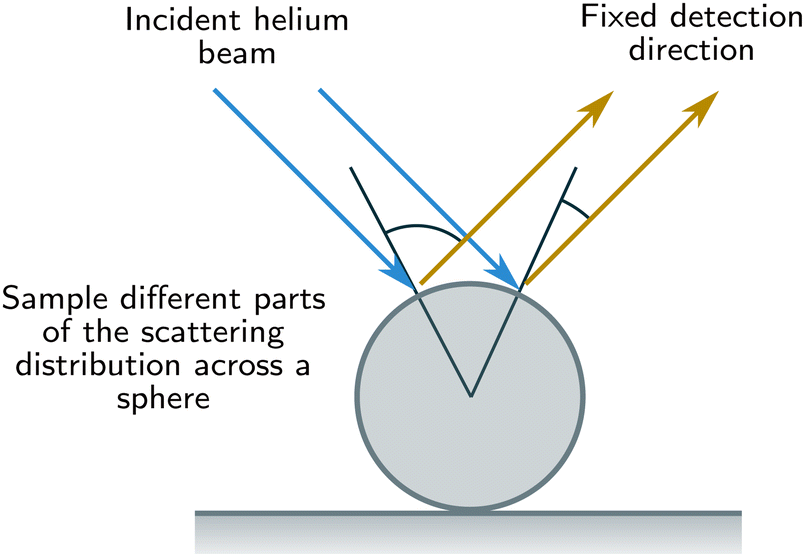
As SHeM instruments are set up to gather data as a function of sample position rather than of detection direction, an alternative approach is taken to acquire scattering distribution information: 2D images of microspheres provide information on many different incidence and detection conditions. The basic concept is presented in Fig. 1, where a helium beam is scanned across a sphere causing the incidence and detection angles to change.
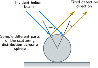 |
| | Fig. 1 Schematic showing that as the helium beam moves across a sphere (shown here in cross-section) the detection and incident angles change, allowing us to gather data on the scattering distribution of the surface of the sample. The concept extends to the whole 3D surface of the sphere. | |
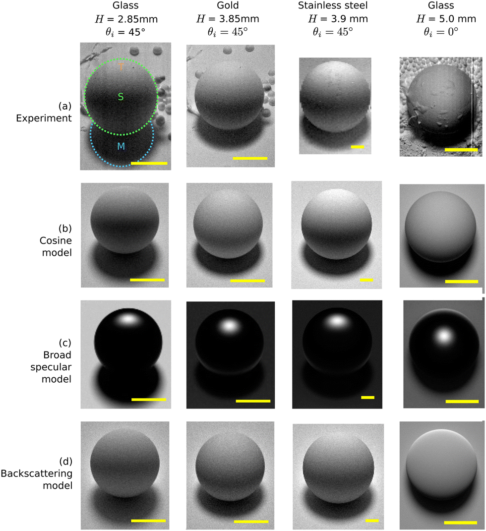
A set of standard glass microspheres‡ were imaged using the University of Cambridge SHeM in three diameters (50 μm, 100 μm, 400 μm), both with and without a thin sputtered gold coating. In addition, complimentary data was taken using the University of Newcastle SHeM on large (∼1 mm diameter) stainless steel spheres as an independent measurement.42 The 50 μm and 100 μm diameter spheres are small enough that changes in detection probability due to the height of the sphere above the nominal sample plane can be ignored and therefore can be used for quantitative analysis. However the 400 μm and ∼1 mm spheres are large enough to cause significant changes in detection probability across them (predominantly through solid angle variations of the detector aperture across the image) and are therefore most useful in comparison with ray-tracing simulations.
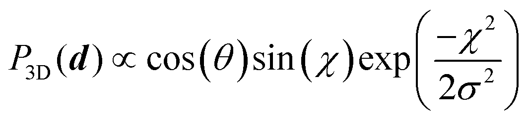
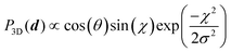
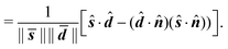
Fig. 2 presents a summary of experimental SHeM images alongside equivalent ray tracing simulations for a range of different conditions. A variety of materials were imaged: the 400 μm glass spheres with and without a thin coating of gold, as well as the 1 mm stainless steel spheres. Additionally, different imaging geometries were used to vary the scattering angles, using either the perpendicular working distance, H, to vary the outgoing detection angle or using a normal incidence beam (rather than the typical θi = 45° geometry) to vary the incidence angle. Projection distortions were accounted for either before or after image collection by scaling the horizontal axis by cos![[thin space (1/6-em)]](https://www.rsc.org/images/entities/char_2009.gif) θi.20 Comparative ray tracing simulations were performed for a pure cosine model, a broad specular distribution and a distribution with a backscattering component. The cosine model is centred on the surface normal and thus has no adjustable parameters. The broad specular model uses a Gaussian centred on the specular condition combined with a cosine term to account for the surface area projection. The probability of scattering in a direction d with an angle χ to the specular condition and an angle θ to the surface normal is,
θi.20 Comparative ray tracing simulations were performed for a pure cosine model, a broad specular distribution and a distribution with a backscattering component. The cosine model is centred on the surface normal and thus has no adjustable parameters. The broad specular model uses a Gaussian centred on the specular condition combined with a cosine term to account for the surface area projection. The probability of scattering in a direction d with an angle χ to the specular condition and an angle θ to the surface normal is,
| |  | (1) |
The distribution has a single parameter
σ, which in the limit of narrow distributions will be the standard deviation of the distribution. A parameter value of
σ = 30° was used, which corresponds to a standard deviation of 24° for the resulting distribution. The backscattering model comprises of a cosine component and an additional component that uses the same form as
eqn (1), except that it is centred on the incidence direction rather than the specular direction.
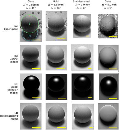 |
| | Fig. 2 (a) Experimental SHeM images of microspheres of different diameters obtained at different perpendicular working distances, H, and incidence angles, θi. Equivalent ray tracing simulations derived for the (b) cosine scattering model, (c) specular scattering model and (d) backscattering model. Scalebars are 200 μm. | |
The experimental SHeM images (Fig. 2a) comprise three distinct SHeM intensity regions: (i) the overall body of the sphere (marked S), (ii) the underlying surface masked from the detector by the sphere (shadow-like feature below the sphere marked M) and (iii) the brighter upper sphere surface (marked T). The relative size of these three regions varies with illumination and thus will be a function of working distance (H), incident angle (θi) and sphere diameter; as observed in the images. Comparison of the experimental data with the corresponding ray-tracing images derived for the cosine-scattering model reveal good qualitative agreement with all four images; reproducing well the observed slowly varying intensity across the surface of the sphere that is weakly peaked towards the detection direction (region T) and the strong contrast that arises from masking of the detector (region M). In contrast, the corresponding ray-tracing images derived for the specular-scattering model all exhibit a characteristic bright reflection ‘spot’ at the top of the sphere that is not seen in the experimental images. Similarly, the ray-tracing image derived for the backscattering model at normal incidence exhibits a bright boundary region at the top of the sphere that again is not observed in the experimental image. Thus, Fig. 2 provides qualitative evidence that the scattered helium follows most closely a slowly varying distribution that is peaked closer to the surface normal than specular. To quantitatively test the level of agreement with a cosine model, the scattering angles across the sphere must be extracted in order to obtain the distribution directly.
4 Quantitative scattering distributions
4.1 Polar relationship
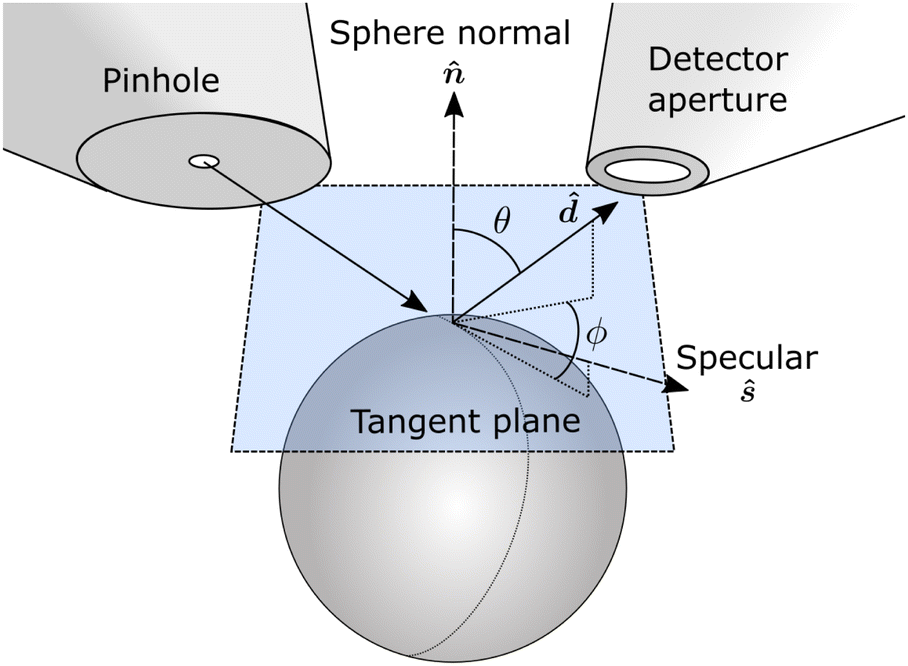
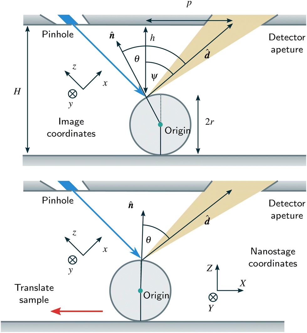
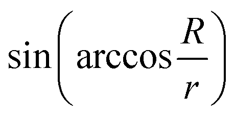
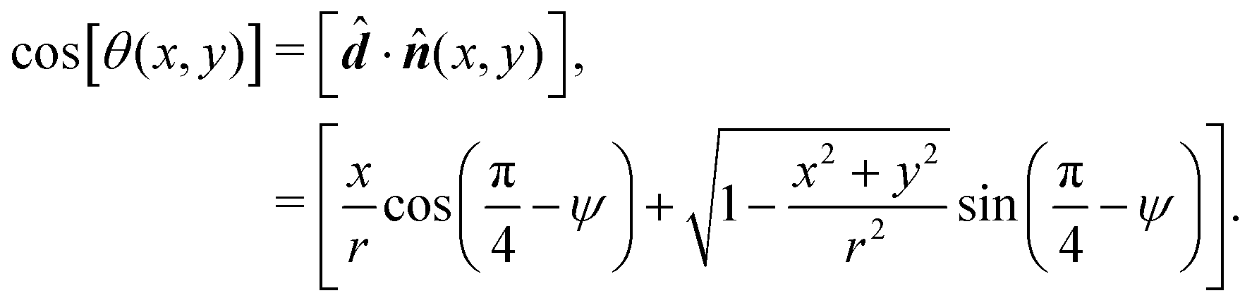
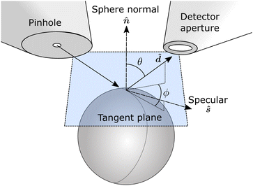
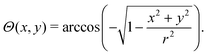
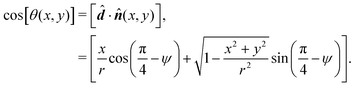
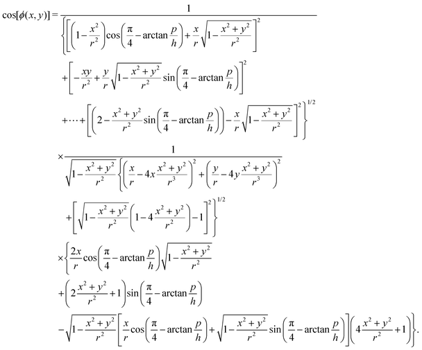
To make quantitative use of data on spheres, the transformation between the coordinates (x,y), in an image need to be converted into the detection polar θ and azimuthal ϕ angles (see Fig. 3). The polar detection angle is| | 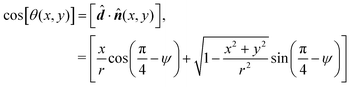 | (2) |
where ψ is the, constant across an image, detection angle for a flat surface, the equation is derived in Appendix A.
 |
| | Fig. 3 Co-ordinate system and vectors used in the derivation of the relation between image positions and incidence and detection angles. d is the vector towards the detector, ![[n with combining circumflex]](https://www.rsc.org/images/entities/b_i_char_006e_0302.gif) is the unit normal to the sphere at the beam-sphere intersection point and ŝ is the vector pointing in the specular reflection direction. is the unit normal to the sphere at the beam-sphere intersection point and ŝ is the vector pointing in the specular reflection direction. | |
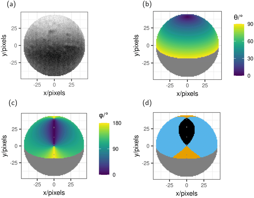
A helium micrograph of a sphere has been isolated in Fig. 4(a) and the corresponding polar angle, θ, is labelled in panel (b) to demonstrate the process of extracting the information associated with each pixel in the sphere image.
 |
| | Fig. 4 The angles of detection across a microsphere image. (a) A SHeM image of a sphere plotted as a function of the pixels (x,y). (b) A heatmap of the polar detection angle θ. (c) The azimuthal detection angle, ϕ. (d) The sphere separated in regions of forwards (black), backwards (orange) and out of plane (blue) scattering. The grey regions do not have direct line of sight to the detector and so are excluded from the analysis. | |
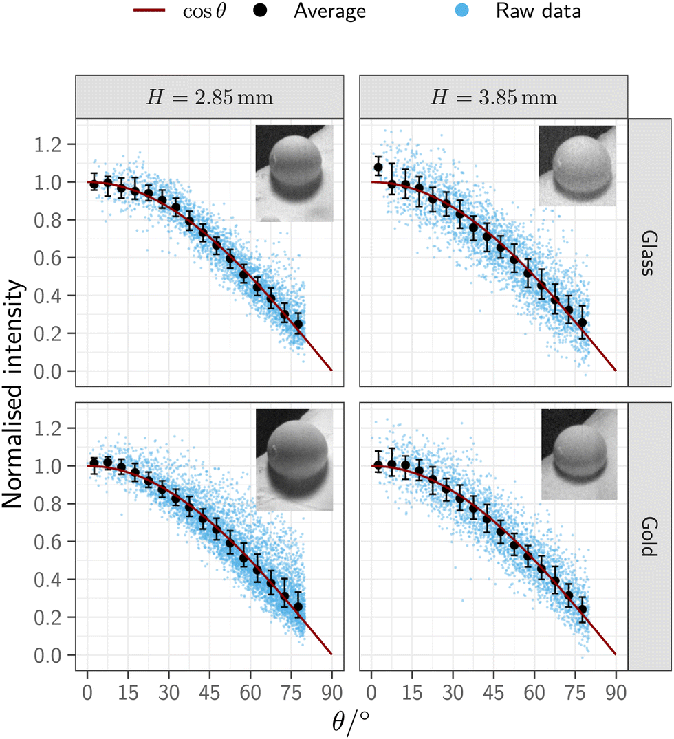
Fig. 5 plots the extracted scattering distribution as a function of the polar detection angle, θ, for a 100 μm glass sphere imaged at two different working distances, H, both with and without a gold coating. The results clearly demonstrate the broad nature of the underlying scattering distribution with atoms being sent into trajectories at all possible outgoing polar angles. In fact, the experimental points are in close agreement with a cos(θ) distribution, shown by the orange line. Therefore, we conclude that diffuse scattering is occurring giving a broad, cosine-like, angular distribution that is peaked near to the surface normal.
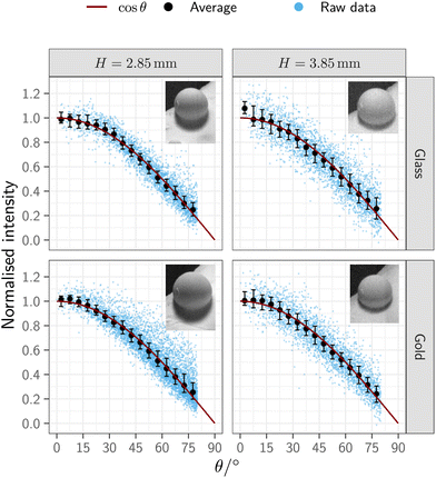 |
| | Fig. 5 Extracted scattering distributions from the 100 μm sphere both with and without gold coating, with insets showing the SHeM images the data was extracted from. The data is normalised by removing the background then scaled so that the fitted cosine has an amplitude of unity. It is clear that the atoms are scattered in a broad diffuse distribution with a stronger tendency for scattering close to the surface normal. | |
4.2 Azimuthal dependence
While there is a good agreement between the extracted scattering distribution and a cosine-like model, it is possible that there is an azimuthal bias within the data that was not visible in Fig. 5. The azimuthal detection angle is derived in Appendix A to be| | 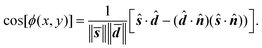 | (3) |
The azimuthal angle, ϕ, across a sphere is plotted in Fig. 4(c). Although ϕ is a continuous variable, for the purposes of the current work the azimuthal detection angle is split into three regions to simplify the discussion. We consider forwards scattering where the atoms scatter largely towards the specular direction; backwards scattering where the atoms scatter towards the incidence direction; and out of plane scattering, where the atoms scatter in between the incidence and specular directions. Mathematically these regions are defined by,| | | |ϕ| < 45°, forwards scattering | (4) |
| | | |ϕ| > 135, backwards scattering | (5) |
| | | 45° < |ϕ| < 135°, out of plane scattering. | (6) |
These three regions of the azimuthal angle, ϕ, are plotted on a sphere in Fig. 4(d).
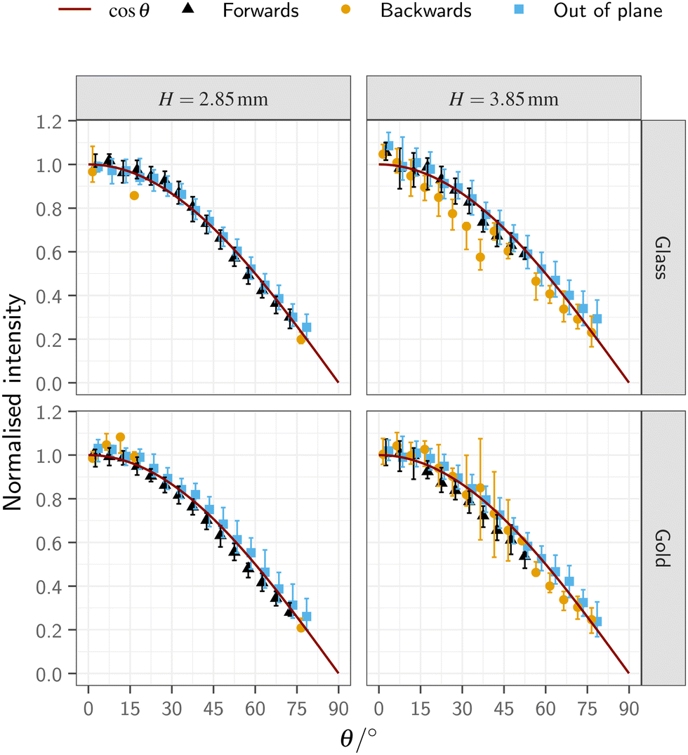
Fig. 6 presents the extracted scattering distribution, allowing for variation between different azimuths as described above, again compared with a cosine distribution. Overall there is still good agreement with the cosine model, with the peak in the distribution being close to the surface normal. None of the data sets show evidence of a backscattering component to the distributions.
 |
| | Fig. 6 Extracted scattering distributions from a 100 μm sphere both with and without gold coating, with a distinction being drawn between ‘forwards’, ‘backwards’ and ‘out of plane’ scattering as defined in eqn (6). The data is normalised by removing the background then scaled so that the fitted cosine has an amplitude of unity. Little difference is seen between the different azimuthal directions, indicated that there is good agreement with the cosine model. | |
5 Discussion
The results show that for the different microsphere material surfaces and helium scattering geometries explored in this work, the SHeM images are best described by a surface-normal centred, approximately cosine-shaped, scattering distribution. Indeed, the wide range of SHeM images reported in the literature7,14,20,21,23,24,26,27,41 can all be qualitatively understood in terms of a cosine-like scattering distribution coupled with local topographic variations in the surface to give rise to the basic image contrast. The contrast is then further enhanced by masking, macroscopic sample height and other secondary effects. As such, this work provides a justification for the use of a cosine-like scattering distribution in ray tracing simulations.21,22 In particular, several images can be collected at different angles to determine the local surface orientation, enabling reconstruction of the complete three dimensional topography of a surface through the heliometric stereo method.43
Observing a cosine-like diffuse scattering mechanism provides insight into the state of the surface of a technological sample. The complete ‘loss of memory’ of the atom's initial trajectory after scattering could be explained through either roughness on a length-scale comparable to the wavelength of the helium beam (∼0.05 nm), a strongly inelastic scattering event, or most likely a combination of both. Therefore, these surfaces must deviate significantly from the perfect crystal surfaces typically studied using HAS. In particular, when comparing the measurements collected in a SHeM to a HAS instrument, the pressure difference between UHV and HV means there will be a greater abundance of contaminants on the surface that are likely to contribute to the observed diffuse scattering. Given the early stage of development and interpretation of the SHeM technique it is difficult to make specific conclusions about the mechanisms that underpin the scattering distribution. Indeed, the data presented here demonstrates that there is considerable opportunity for collaboration between experimental and theoretical groups, to develop the energy resolved measurements and associated in-depth theory required to fully describe the phenomenon.
Deviations from simple cosine-scattering have already been observed, such as the case of dissimilar metal films on silicon, implying that surfaces that are nominally flat can also exhibit contrast differences in SHeM.27 Therefore, while technological surfaces generally exhibit cosine-like scattering distributions, further work is needed to understand and exploit these deviations to extract information about the surface. Looking forward, we expect it to be possible to determine both the contamination state and even changes in nanoscale topography of many surfaces.
6 Conclusions & outlook
By analysing SHeM images of various microspheres, we have established that the atoms scattered from unprepared ‘technological’ samples in a scanning helium microscope follow an approximate cosine distribution centred around the local surface normal direction. These observations are consistent with a wide range of helium images now in the scientific literature, collectively demonstrating cosine-like scattering distributions should be generally expected in SHeM. These distributions represent a marked contrast with traditional HAS experiments on pristine surfaces where very different distributions are observed, reflecting the atomic structure and dynamics of the surface, and demonstrate how the development of SHeM is now pushing the limits of understanding within the traditional boundaries of atom–surface scattering.
Importantly, these observations establish a firm basis for both qualitative and quantitative interpretation of typical SHeM images, on the basis of a dominant topographic mechanism which can be supplemented by, and form a reference to compare to, other contrast effects. Our observations also raise new and exciting questions at a theoretical level, specifically relating to understanding the atomic scale origin of the cosine-distribution effect, its generality and the point at which approximation breaks down – which will all be crucial for the future quantitative analysis and interpretation in the field of helium microscopy.
Author contributions
SML, MBe, DJW, JE, and APJ conceptualised the investigation and the experiments. SML, MBe and AR performed the Cambridge SHeM experiments. MBa, AF and TM performed the Newcastle SHeM measurements. SML performed the ray tracing simulations and the data analysis. MBe assisted in preliminary data analysis. APJ, JE and PD supervised the project. SML, MBe, DJW and APJ prepared the manuscript. All authors discussed the results and reviewed the manuscript.
Conflicts of interest
There are no conflicts to declare.
A Derivation of transformation
In order to make quantitative use of data on spheres, the relationship between the coordinates, x,y, in an image need to be converted into the incidence angle Θ and the detection polar and azimuthal angles θ,ϕ. A vector approach is taken in the native coordinate system of the image projection, x,y, which has the z axis parallel to the incidence beam. The derivation of the relationships assumes that the sphere is small and therefore changes to the detection conditions across the sphere are negligible.
The Cartesian coordinate system used is shown in Fig. 7, relative to the spherical sample and the basic instrument geometry, with the z axis parallel to the beam making the (x,y) coordinates equivalent, up to a linear transformation, to the coordinates of the nano-stage motion: (x = XcosΘ,Y = y). In this coordinate system, assuming spheres of negligible size, there is a constant vector to the detector, ![[d with combining circumflex]](https://www.rsc.org/images/entities/b_i_char_0064_0302.gif) , and the quantity that must be derived is the local normal vector of the sphere (x,y).
, and the quantity that must be derived is the local normal vector of the sphere (x,y).
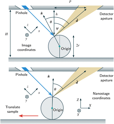 |
| | Fig. 7 Co-ordinate system and vectors used in the derivation of the relation between image positions and incidence and detection angles. d is the vector towards the detector, and is the unit normal to the sphere at the beam-sphere intersection point. The coordinate system is defined to have the z axis parallel to the beam and the origin at the centre of the sphere. The distance from the scattering point to the pinhole plate h does vary across the sphere but can be neglected for small enough spheres. | |
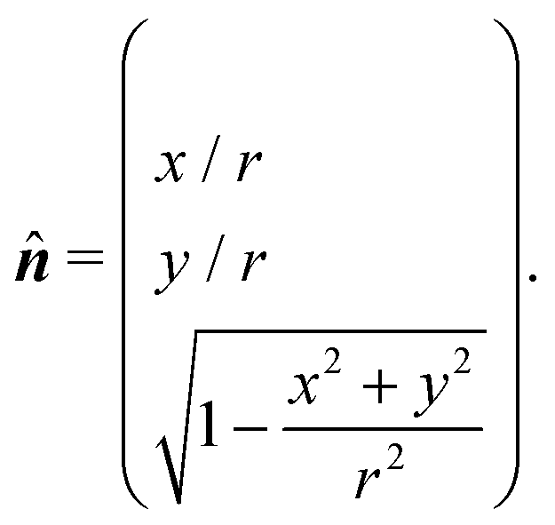
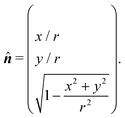
Consider a sphere of radius r, with its centre on the origin, as shown in Fig. 7. At a distance R from the centre of the sphere, on the positive z hemisphere, the unit normal will have a component in z of magnitude
| |  | (7) |
and a component in the (
x,
y) plane radially away from the centre of the sphere of
R/
r. Therefore, we can write the normal vector as,
| |  | (8) |
Next, the vector from the sphere to the detector needs to be acquired. Using the variables from
Fig. 7,
| | 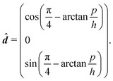 | (9) |
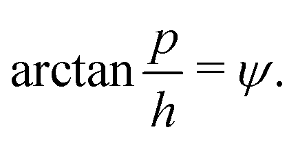
Note that the ‘overall’ detection angle
ψ is found
via| |  | (10) |
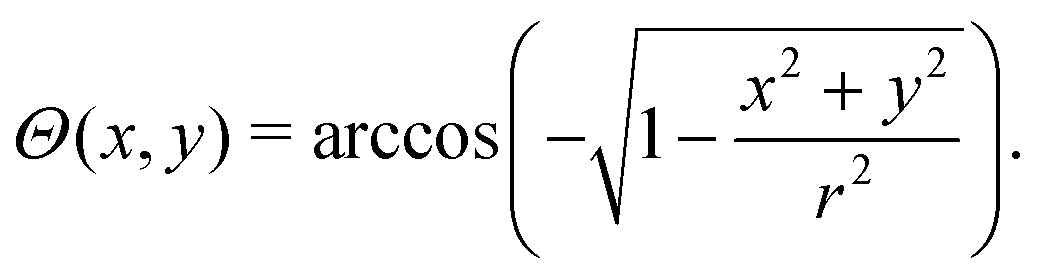
A full description of the scattering distribution is a function of the incident angle to the surface, which can be calculated using the local surface normal in
eqn (8) and the incident beam direction given in the native coordinate system of the image as,
thus the incidence polar angle,
Θ is
| |  | (12) |
Assuming that the surface is isotropic, it is possible to ignore the incident azimuthal angle,
Φ. The outgoing polar angle is then given by,
| |  | (13) |
Finally the outgoing azimuthal angle, ϕ, which is the angle between the specular direction and the detector direction must be computed. The specular direction is given by subtracting twice the projection of the incidence direction onto the surface normal,
| | | ŝ = ê − 2(ê·) | (14) |
and the azimuthal angle is the angle between the
and
ŝ vectors after projection onto the plane normal to
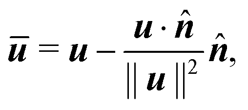
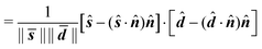
(also the tangent plane of the sphere through the scattering point). Projection onto the plane can be performed by subtracting the component of the vector that is parallel to the normal vector. Using bar to denote the projected vectors,
| | 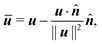 | (15) |
which must then be normalised, gives the azimuthal angle as
| | cos[ϕ(x,y)] = ![[s with combining macron]](https://www.rsc.org/images/entities/b_i_char_0073_0304.gif) · ·![[d with combining macron]](https://www.rsc.org/images/entities/b_i_char_0064_0304.gif) | (16) |
| |  | (17) |
| |  | (18) |
Thus the scattering distribution information can be derived from a SHeM image of a sphere. The general scattering distribution that can be obtained is a function of three variables, I(Θ,θ,ϕ) and it should be noted that only a small part of the total space will be sampled. However the result can be directly compared to potential models of scattering.
The transform for the outgoing azimuthal angle can be written out explicitly in terms of the image coordinates thus:
| |  | (19) |
Acknowledgements
The work was supported by EPSRC grant EP/R008272/1. The authors acknowledge support by the Cambridge Atom Scattering Centre (https://atomscattering.phy.cam.ac.uk) and EPSRC award EP/T00634X/1. SML acknowledges funding from Mathworks Ltd. The work was performed in part at the Materials node of the Australian National Fabrication Facility, a company established under the National Collaborative Research Infrastructure Strategy to provide nano and microfabrication facilities for Australias researchers.
References
-
B. Poelsema and G. Comsa, Scattering of Thermal Energy Atoms, from Disordered Surfaces, Springer, 1st edn, 1989 Search PubMed.
-
E. Hulpke, Helium Atom Scattering from Surfaces, Springer, 1st edn, 1992 Search PubMed.
- D. Farias and K.-H. Rieder, Rep. Prog. Phys., 1998, 61, 1575 CrossRef CAS.
-
G. Benedek and J. P. Toennies, Atomic Scale Dynamics at Surfaces, Theory and Experimental Studies with Helium Atom Scattering, Springer, 1st edn, 2018 Search PubMed.
- G. Benedek, J. R. Manson and S. Miret-Artés, Phys. Chem. Chem. Phys., 2021, 23, 7575–7585 RSC.
- B. Holst, G. Alexandrowicz, N. Avidor, G. Benedek, G. Bracco, W. E. Ernst, D. Farías, A. P. Jardine, K. Lefmann, J. R. Manson, R. Marquardt, S. M. Artés, S. J. Sibener, J. W. Wells, A. Tamtögl and W. Allison, Phys. Chem. Chem. Phys., 2021, 23, 7653–7672 RSC.
- M. Barr, A. Fahy, A. Jardine, J. Ellis, D. Ward, D. MacLaren, W. Allison and P. Dastoor, Nucl. Instrum. Methods Phys. Res., Sect. B, 2014, 340, 76–80 CrossRef CAS.
- P. Witham and E. Sánchez, Rev. Sci. Instrum., 2011, 82, 103705 CrossRef PubMed.
- S. D. Eder, T. Reisinger, M. M. Greve, G. Bracco and B. Holst, New J. Phys., 2012, 14, 073014 CrossRef.
- S. D. Eder, X. Guo, T. Kaltenbacher, M. M. Greve, M. Kalläne, L. Kipp and B. Holst, Phys. Rev. A: At., Mol., Opt. Phys., 2015, 91, 043608 CrossRef.
- S. D. Eder, A. K. Ravn, B. Samelin, G. Bracco, A. S. Palau, T. Reisinger, E. B. Knudsen, K. Lefmann and B. Holst, Phys. Rev. A, 2017, 95, 023618 CrossRef.
- M. Koch, S. Rehbein, G. Schmahl, T. Reisinger, G. Bracco, W. E. Ernst and B. Holst, J. Microsc., 2008, 229, 1–5 CrossRef CAS PubMed.
- D. A. MacLaren, B. Holst, D. J. Riley and W. Allison, Surf. Rev. Lett., 2003, 10, 249–255 CrossRef CAS.
- T. A. Myles, S. D. Eder, M. G. Barr, A. Fahy, J. Martens and P. C. Dastoor, Sci. Rep., 2019, 9, 2148 CrossRef PubMed.
- G. Bhardwaj, K. R. Sahoo, R. Sharma, P. Nath and P. R. Shirhatti, Phys. Rev. A, 2022, 105, 022828 CrossRef CAS.
- M. Bergin, S. M. Lambrick, H. Sleath, D. J. Ward, J. Ellis and A. P. Jardine, Sci. Rep., 2020, 10, 1–8 CrossRef PubMed.
- M. Bergin, D. J. Ward, J. Ellis and A. P. Jardine, Ultramicroscopy, 2019, 112833 CrossRef CAS PubMed.
- A. S. Palau, G. Bracco and B. Holst, Phys. Rev. A, 2016, 94, 063624 CrossRef.
- A. Salvador Palau, G. Bracco and B. Holst, Phys. Rev. A, 2017, 95, 013611 CrossRef.
- A. Fahy, S. D. Eder, M. Barr, J. Martens, T. A. Myles and P. C. Dastoor, Ultramicroscopy, 2018, 192, 7–13 CrossRef CAS PubMed.
- S. M. Lambrick, L. Vozdecký, M. Bergin, J. E. Halpin, D. A. MacLaren, P. C. Dastoor, S. A. Przyborski, A. P. Jardine and D. J. Ward, Appl. Phys. Lett., 2020, 116, 061601 CrossRef CAS.
- S. M. Lambrick, M. Bergin, A. P. Jardine and D. J. Ward, Micron, 2018, 113, 61–68 CrossRef CAS PubMed.
- T. A. Myles, A. Fahy, J. Martens, P. C. Dastoor and M. G. Barr, Measurement, 2020, 151, 107263 CrossRef.
- A. Fahy, M. Barr, J. Martens and P. C. Dastoor, Rev. Sci. Instrum., 2015, 86, 023704 CrossRef CAS PubMed.
- P. Witham and E. Sánchez, Cryst. Res. Technol., 2014, 49, 690–698 CrossRef CAS.
- P. J. Witham and E. J. Sánchez, J. Microsc., 2012, 248, 223–227 CrossRef CAS PubMed.
- M. Barr, A. Fahy, J. Martens, A. P. Jardine, D. J. Ward, J. Ellis, W. Allison and P. C. Dastoor, Nat. Commun., 2016, 7, 10189 CrossRef CAS PubMed.
-
S. M. Lambrick, PhD thesis, University of Cambridge, 2021.
- F. E. Nicodemus, Appl. Opt., 1965, 4, 767–775 CrossRef.
- B. Holst and W. Allison, Nature, 1997, 390, 244 CrossRef CAS.
- S. Miret-Artés and E. Pollak, Surf. Sci. Rep., 2012, 67, 161–200 CrossRef.
- G. Benedek and J. P. Toennies, Surf. Sci., 1994, 299–300, 587–611 CrossRef CAS.
- J. Boheim and W. Brenig, Z. Phys. B: Condens. Matter, 1981, 41, 243–250 CrossRef.
- R. Feres and G. Yablonsky, Chem. Eng. Sci., 2004, 59, 1541–1556 CrossRef CAS.
- F. Borondo, C. Jaffé and S. Miret-Artés, Surf. Sci., 1994, 317, 211–220 CrossRef CAS.
-
M. Knudsen, The kinetic theory of gases: some modern aspects, 3rd edn, 1950 Search PubMed.
-
Photometria sive de mensura et gradibus luminis, colorum et umbrae, Augustae Vindelicorum, Augsburg, 1760.
- B. v Ginneken, M. Stavridi and J. J. Koenderink, Appl. Opt., 1998, 37, 130–139 CrossRef PubMed.
- T. S. Hegge, T. Nesse, A. A. Maradudin and I. Simonsen, Wave Motion, 2018, 82, 30–50 CrossRef.
- D. R. O’Keefe and R. L. Palmer, J. Vac. Sci. Technol., 1971, 8, 27–30 CrossRef.
-
M. Bergin, PhD thesis, Fitzwilliam College, University of Cambridge, 2018.
-
M. Barr, Imaging with atoms: aspects of scanning helium microscopy, PhD thesis, University of Newcastle, 2016 Search PubMed.
- S. M. Lambrick, A. Salvador Palau, P. E. Hansen, G. Bracco, J. Ellis, A. P. Jardine and B. Holst, Phys. Rev. A, 2021, 103, 053315 CrossRef CAS.
Footnotes |
| † A supporting data pack for this work, containing the raw data used to produce the presented scattering distributions, can be found in the University of Cambridge data repository at DOI: https://doi.org/10.17863/CAM.87438. |
| ‡ The spheres were Monodisperse Standards from Whitehouse Scientific, MS0009, MS0026, MS0049, MS0114 & MS0406, https://www.whitehousescientific.com/category/monodisperse-standards?c341c912_page=2. |
|
| This journal is © the Owner Societies 2022 |
Click here to see how this site uses Cookies. View our privacy policy here. 
 Open Access Article
 This Open Access Article is licensed under a
  *a,
M.
Bergin
*a,
M.
Bergin