
 Open Access Article
 This Open Access Article is licensed under a
 Creative Commons Attribution 3.0 Unported Licence
Topological fine structure of smectic grain boundaries and tetratic disclination lines within three-dimensional smectic liquid crystals
Paul A.
Monderkamp
 a,
René
Wittmann
*a,
Michael
te Vrugt
b,
Axel
Voigt
c,
Raphael
Wittkowski
b and
Hartmut
Löwen
a
a,
René
Wittmann
*a,
Michael
te Vrugt
b,
Axel
Voigt
c,
Raphael
Wittkowski
b and
Hartmut
Löwen
a
aInstitut für Theoretische Physik II: Weiche Materie, Heinrich-Heine-Universität Düsseldorf, 40225 Düsseldorf, Germany. E-mail: rene.wittmann@hhu.de
bInstitut für Theoretische Physik, Center for Soft Nanoscience, Westfälische Wilhelms-Universität Münster, 48149 Münster, Germany
cInstitut für Wissenschaftliches Rechnen, Technische Universität Dresden, 01062 Dresden, Germany
First published on 5th May 2022
Abstract
Observing and characterizing the complex ordering phenomena of liquid crystals subjected to external constraints constitutes an ongoing challenge for chemists and physicists alike. To elucidate the delicate balance appearing when the intrinsic positional order of smectic liquid crystals comes into play, we perform Monte-Carlo simulations of rod-like particles in a range of cavities with a cylindrical symmetry. Based on recent insights into the topology of smectic orientational grain boundaries in two dimensions, we analyze the emerging three-dimensional defect structures from the perspective of tetratic symmetry. Using an appropriate three-dimensional tetratic order parameter constructed from the Steinhardt order parameters, we show that those grain boundaries can be interpreted as a pair of tetratic disclination lines that are located on the edges of the nematic domain boundary. Thereby, we shed light on the fine structure of grain boundaries in three-dimensional confined smectics.
1 Introduction
Omnipresent throughout a vast range of chemical and physical systems,1–12 topological defects play a central role in characterizing collective ordering phenomena. As one of the default systems for investigating such ordering phenomena, liquid crystals13 have been enjoying continuous attention within the physical chemistry and chemical physics communities over the past decades and remain an active field of research.14 Liquid-crystalline mesophases accompanied by topological defects occur, e.g., in viral colonies,15 bacterial DNA,16 biopolymers,17 and active systems18–21 realized, e.g., by swarms of bacteria22–25 or driven filaments.26,27 Topological analysis even provides a tool for insight into the collective behavior of animals on a macroscopic scale, e.g., shoals of fish, where local coherent swimming is a vital tool in the evasion of predators.28,29The most prominent type of ordering, which is typically found in liquid crystals, is orientational (nematic) ordering, where the characteristically shaped subunits, i.e., molecules or colloidal particles in close proximity, show a tendency to align. This alignment can be induced or enhanced by the system boundaries.30–32 If the nematic order gets frustrated, e.g., within floating droplets,33–37 by external confinement,38–48 near obstacles,49–58 or on curved surfaces,59–65 topological defects emerge, which are discontinuities in the ordered structures that can display particle-like properties themselves.1,20,66–68
In liquid crystals which feature exclusively orientational order of the fluid particles, so-called nematics, the commonly observed stable defects are singular points in a two-dimensional (2d) plane and curves in three-dimensional (3d) space that are either closed or end on system boundaries. The defect strength in 2d nematic liquid crystals is characterized by a so-called topological charge, which obeys an additive conservation law in analogy to the electric charge. This topological charge is determined by the total change of the preferred local orientation of the fluid on a contour around the defects.69,70 At higher densities and/or low temperatures, certain liquid crystals form the so-called smectic phase, which additionally displays positional order. Traditionally, the study of defects in smectic liquid crystals is mainly concerned with the purely positional defects, such as edge dislocations71–74 or complex structures like focal conics.75–77 However in situations, where frustration of nematic ordering takes a pronounced role, the consideration of the topology of the local orientations has proven insightful.
Smectic liquid crystals are characterized by an intrinsic layering, such that the discontinuities in the local order preferably appear as grain boundaries separating different domains within the fluid. These elongated defects possess a linear shape in two and a planar shape in three dimensions.78 The formation of grain boundaries can be enforced when the fluid is confined to a container, such that the local preferred orientation in the system depends heavily on the position. This is in particular the case for colloidal liquid crystals which interact mainly through volume exclusion and possess a strong tendency to maintain a uniform layering, such that the relaxation of external constraints by elastic deformations only plays a minor role (unless favored by the confining topology).79 For such 2d colloidal liquid crystals, we have previously elaborated that the notion of the emerging domain boundaries as topological objects with coexisting nematic and tetratic charges yields insight into the orientational topology of smectics80 (for a comprehensive summary see Section 2.3). However, the role of the orientations within smectic liquid crystals still remains to be further understood. This concerns in particular the analysis of three-dimensional systems.
To shed more light on this issue, we present a range of simulation results for confined hard rods, representing colloidal smectic liquid crystals in three dimensions. The confinement causes frustration of the bulk symmetry and induces the formation of topological defects, which are observed and analyzed on the particle scale by treating the local orientations of the rods as indicative of the local director field. As elaborated in Section 2.3, the investigation of orientational topology in three dimensions is more involved, since 3d topological charges do not adhere to an additive charge conservation like their 2d counterparts.69,81 However, under specific circumstances, this additive charge conservation is recovered. By elaborating on the analogy to the 2d case, we explain the effects of the introduction of the third dimension and investigate the conditions for additive topological charge conservation.
This article is structured as follows: in Section 2, we present our methodology. After elaborating in Section 2.1 on the simulation protocol, we introduce the order parameters used to characterize the simulation results in Section 2.2, while we provide a detailed discussion of the three-dimensional tetratic order parameter in Appendix A. In Section 2.3, we explain the analysis of the topological charge and the details of the charge conservation. In Section 3, we present our results, by first evaluating in Section 3.1 the order parameters to detect and classify the emerging defects in our particle-resolved snapshots. Then we characterize the layer structure and orientations within the two confinements in Section 3.2, where Appendix B provides more detailed account of the cylindrical geometry. We discuss the implications on the topological charge in Section 3.3. Lastly, we conclude in Section 4.
2 Methods
2.1 Simulations
We perform canonical Monte Carlo (MC) simulations of a model for colloidal rods confined to 3d cavities, see Fig. 1. Specifically, we consider soft walls in the shape of cylinders {r ∈![[Doublestruck R]](https://www.rsc.org/images/entities/char_e175.gif) 3|rx2 + ry2 ≤ R2, 0 ≤ rz ≤ h} and spherical caps, resembling a drop-like shape, {r ∈ 3|rx2 + ry2 + rz2 < R2, rz > R − h}, both of radius R and height h. The rods are modeled as hard spherocylinders with aspect ratio p = L/D = 5, with core length L and diameter D. Note that in two dimensions, one would require significantly longer rods to observe stable smectic structures.
3|rx2 + ry2 ≤ R2, 0 ≤ rz ≤ h} and spherical caps, resembling a drop-like shape, {r ∈ 3|rx2 + ry2 + rz2 < R2, rz > R − h}, both of radius R and height h. The rods are modeled as hard spherocylinders with aspect ratio p = L/D = 5, with core length L and diameter D. Note that in two dimensions, one would require significantly longer rods to observe stable smectic structures.
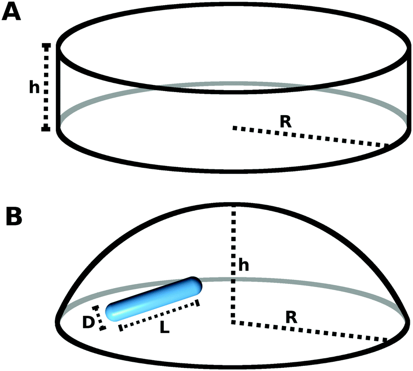 | ||
| Fig. 1 Schematic depiction of the confinement considered in our simulation of three-dimensional liquid crystals. We simulate the liquid crystals by a system of N spherocylinders with length L and diameter D in confinement to suppress the bulk symmetry of the fluid in order to observe topological defects. (A) Cylindrical cavity with radius R and height h. (B) Spherical-cap cavity with radius R and height h. | ||
The pair potential for the particle–particle interaction is given by the standard hard-core repulsion82
 | (1) |
 | (2) |
 | (3) |
 | (4) |
To create the smectic structures in our 3d cavities, we follow a compression protocol, where we initialize the system at a low volume fraction η0 = 5 × 10⁻³ and compress until the volume fraction η2 = 0.52 is reached, at which the smectic-A phase is stable in the bulk. Here, the volume fraction η is defined as η = NVhsc/Vcav, with the particle number N, the volume of a hard spherocylinder Vhsc and the total volume of the confining cavity Vcav. Since in each simulation run the particle geometry, the shape and size of the confinement and the final volume fraction are fixed, the particle number N is a variable that gets adjusted accordingly. The values of N we investigate, determined by the parameters above, typically lie between N ≈ 200 for extremely shallow cavities and N ≈ 3300 for the tallest cavities with h = 4.5L that are addressed in the main part of this publication.
After initialization at η0 = 5 × 10⁻³, we perform a large number of MC cycles, each of which consists of a trial displacement or rotation of each particle. The acceptance probability  is given by the Metropolis criterion from the difference ΔU of the energies (see eqn (1) and (3)) in the system before and after trial move.84 In detail, we compress the system for 106 MC cycles ∼109 trial moves with a rate of Δη1 = 2.45 × 10⁻⁷ per MC cycle to the volume fraction η1 = 0.25 and then, in a second stage for 5 × 10⁶ MC cycles ∼5 × 10⁹ trial moves, with a rate Δη2 = 5.4 × 10⁻⁸ per MC cycle to η2 = 0.52. This two-step simulation protocol is implemented such that the majority of the simulation takes place in the regime of the packing fraction where self-assembly into the ordered phases occurs, ensuring a proper equilibration. To calculate average distribution functions and global order parameters, we gather statistics from up to 15 simulation runs.
2.2 Order parameters
We examine the structure of the confined fluid with the help of two orientational order parameters. The first one is the standard nematic order parameter , associated with orientational ordering of uniaxial particles, which corresponds to the largest eigenvalue of the nematic tensor
  .13,85 To numerically generate the scalar field
  , we sample the nematic tensor within a spherical subsystem of radius 2.5D around each point r as
 | (5) |
![[thin space (1/6-em)]](https://www.rsc.org/images/entities/char_2009.gif) θkcosϕk, sinθksinϕk, cosθk)T in spherical coordinates for k ∈ {1,…,NB}, where θ and ϕ are the angles to the z- and x-axes, respectively, and the 3d unit matrix
θkcosϕk, sinθksinϕk, cosθk)T in spherical coordinates for k ∈ {1,…,NB}, where θ and ϕ are the angles to the z- and x-axes, respectively, and the 3d unit matrix ![[Doublestruck I]](https://www.rsc.org/images/entities/char_e16c.gif) 3.
3.  denotes the largest eigenvalue of
  . The mean local orientation
 ![[n with combining circumflex]](https://www.rsc.org/images/entities/b_char_006e_0302.gif) (r) = n(r)/‖n(r)‖ of the rods, i.e., the nematic director, can be computed by normalizing the eigenvector n(r) associated with
(r) = n(r)/‖n(r)‖ of the rods, i.e., the nematic director, can be computed by normalizing the eigenvector n(r) associated with  , where ‖·‖ is the Euclidean norm.
As will be discussed later, the favorable nematic bulk symmetry of orientational ordering is broken when the fluid is confined to a cavity. In two dimensions, the topological fine structure of the spatially extended defect lines in the director field (r) can be investigated using a scalar tetratic order-parameter field, which can be defined as
 | (6) |
 when each pair of rods is either mutually parallel or perpendicular.
Similarly, in three dimensions, the discontinuities in the director field typically form grain boundaries, e.g., defect planes. To develop a classification concept in three dimensions, we construct in Appendix A a 3d tetratic order parameter from the Steinhardt order parameters88
 | (7) |
 is given by
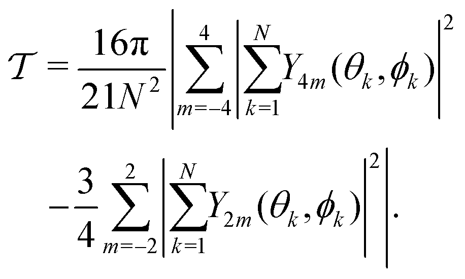 | (8) |
 for an isotropic system, where the orientations {ûk} are uniformly distributed on the unit sphere S2 and
  for a system where all orientations are pairwise either parallel or orthogonal, i.e., if we have a local Cartesian coordinate system, where all rods are aligned to either of the axes. Analogously to the 2d tetratic order parameter
  , our definition (8) of
  implies both perfect cubatic (
 ,
,  ) and perfect nematic order (
 ,
,  ) as special cases of
  , such that we cannot measure this kind of tetratic order in a 3d system with either the standard cubatic89,90 or the standard nematic order parameter.
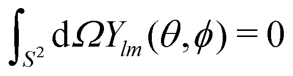
We now prove that the 3d tetratic order parameter (8) has the desired properties. First, we show that it is 0 for an isotropic system. In this case, the orientations {θk, ϕk} approach a uniform distribution on the unit sphere S2, such that the inner sums over k in eqn (8) approach an integral over S2. This integral vanishes since the spherical harmonics satisfy
 | (9) |
 is by construction invariant under coordinate transformations and since the functions Y4m and Y2m are invariant under parity transformation, we can assume without loss of generality that we have a configuration (Λ) of a particles with orientation (θ,ϕ) = (π/2, 0), b particles with orientation (θ,ϕ) = (π, 0) and c particles with orientation (θ,ϕ) = (π/2, π/2) (with a, b, c ∈
 ![[Doublestruck N]](https://www.rsc.org/images/entities/char_e171.gif) 0). The order parameter (8) then evaluates to
0). The order parameter (8) then evaluates to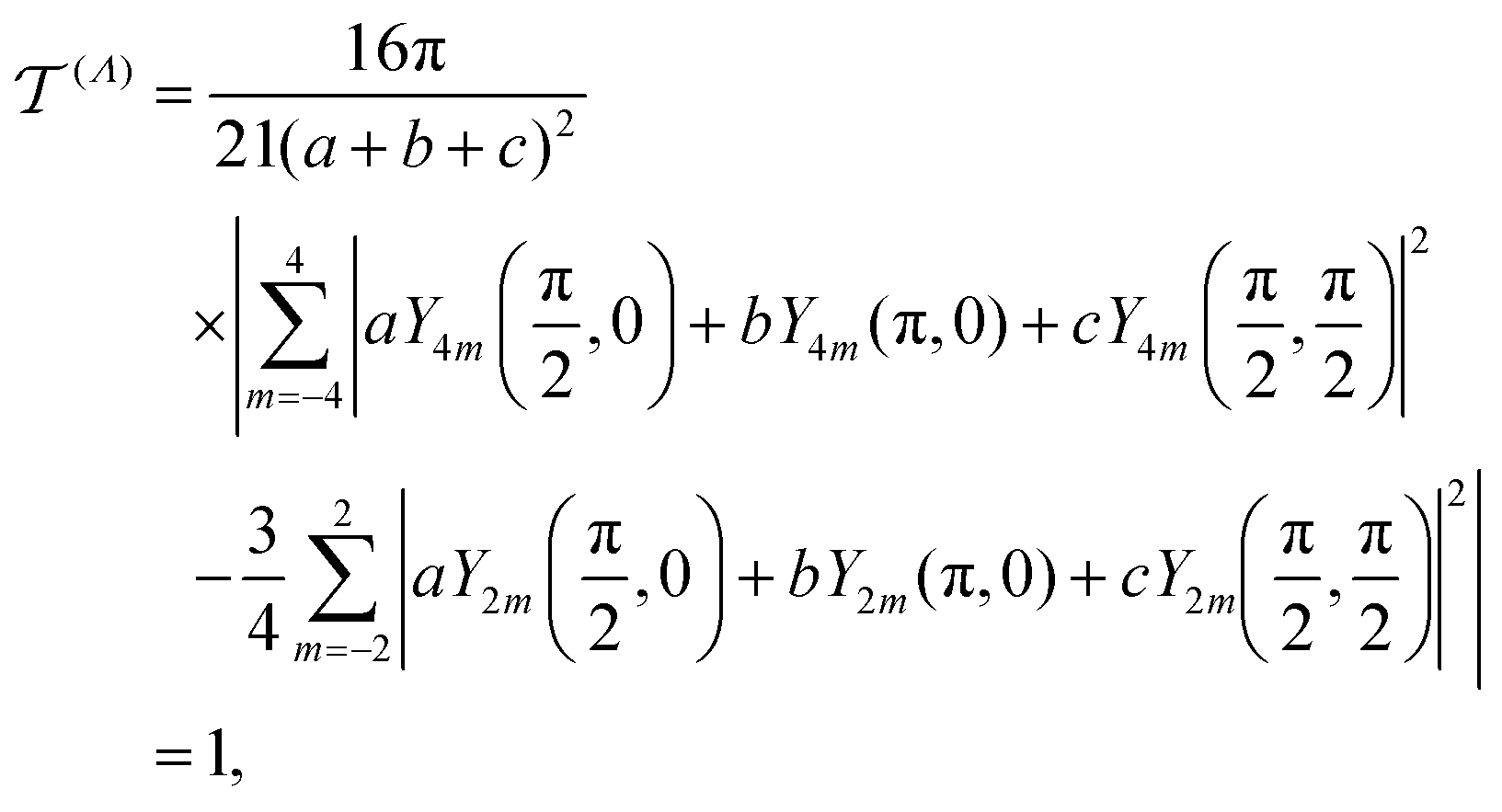 | (10) |
Finally, to generate a local field  of the tetratic order parameter from our simulation data, we sample the spherical harmonics entering eqn (8) only within local spherical subsystems B2.5D(r), which yields
 | (11) |
2.3 Topological charge
Topological defects are identified as discontinuities in the director field(r), see Fig. 2. In 2d nematic liquid crystals, the types of stable bulk defects are point defects. The strength of the defect, i.e., the degree of deformation of the surrounding fluid, is typically analyzed by a topological charge Q that equates to the total rotation of the director traversing any contour  around the defect. This charge is given by the winding number that can be explicitly calculated as the closed line integral along the contour
  parametrized by κ, i.e.,
 | (12) |
 .85 Due to the apolarity of the particles, the configuration space of the orientations is a semicircle with end points identified, commonly denoted by S1/Z2, i.e., we now consider to be a headless vector in the sense that we identify and −.
 | ||
| Fig. 2 Schematic of the classification of topological defects in two dimensions, present as discontinuities in the director field (r). The topological charge of a defect corresponds to the net rotation of (r) traversing the defect in counter-clockwise direction (indicated by the arrow in A1) around the defects. (A) Point defects for particles of π rotational symmetry with charges Q = +1/2 (A1) and Q = −1/2 (A2) typically present in nematic liquid crystals. (B) Decomposition of smectic grain boundaries into tetratic point defects. Due to the preferred difference in orientation angles of π/2, the line defects can be classified as two isolated tetratic point defects of charge q = ±1/4. The schematic shows an exemplary line defect of total charge Q = q1 + q2 = 1/2. (C) Point defects for particles with π/2 rotational symmetry. Charges are q = +1/4 (C1) and q = −1/4 (C2). For ease of observing the continuous rotation, the two main axes are decorated differently. | ||
From a topological point of view, we define the charge via the winding number because (since the winding number is a discrete quantity) different contours with different winding numbers can not be continuously transformed into each other, i.e., are not homotopic. All possible contours in the liquid crystal correspond to loops in S1/Z2. The fundamental group π1(S1/Z2) classifies loops in S1/Z2 up to homotopy equivalence. Consequently, all possible defects are classified by the fundamental group π1(S1/Z2). This group is given by  with the addition operation +. (The prefactor 1/2 is a convention used in physics that is motivated by the geometric definition of charges via the winding number.) Therefore, the possible charges are Q ∈ {k/2|k ∈
 ![[Doublestruck Z]](https://www.rsc.org/images/entities/char_e17d.gif) } and these charges can be added to find the total charge of a combination of two defects. The sum of all charges is a conserved quantity in two dimensions (since it has to match the Euler characteristic of the confinement91). As an example, we illustrate Q = 1/2 in Fig. 2A1 and Q = −1/2 in Fig. 2A2. Moreover, the number of elements in π1(S1/Z2) is infinite, which is exemplified by the fact that the winding number can be any half-integer.
} and these charges can be added to find the total charge of a combination of two defects. The sum of all charges is a conserved quantity in two dimensions (since it has to match the Euler characteristic of the confinement91). As an example, we illustrate Q = 1/2 in Fig. 2A1 and Q = −1/2 in Fig. 2A2. Moreover, the number of elements in π1(S1/Z2) is infinite, which is exemplified by the fact that the winding number can be any half-integer.
Defects typically observed in 3d nematics are disclination lines, along which the local orientational order is frustrated. (Point defects in three dimensions (hedgehogs) are not considered in this work.) In analogy to the 2d case, topological defects can be classified by considering closed loops in the orientational configuration space, up to homotopy equivalence. One typically analyses the defect in terms of the topology of a planar cross-section perpendicular to the disclination line.92 Since the configuration space of the orientations in three dimensions is a hemisphere with antipodal points identified, commonly denoted by S2/Z2, the rotation of (r) along  forms loops in S2/Z2, classified by π1(S2/Z2). By rotation into the third dimension, all half-integer disclinations can be continuously mapped onto each other. Correspondingly, π1(S2/Z2) has only two elements. As a result, for instance, 3d defects with cross-sections like in Fig. 2A1 (Q = +1/2) and Fig. 2A2 (Q = −1/2) are homotopically equivalent. More specifically, the opposite charges ±1/2 correspond to opposite paths around half of the base of the hemisphere S2/Z2, both connecting two antipodal points. A +1/2 defect can be transformed into a −1/2 defect by passing the corresponding path in S2/Z2 over the north pole of the hemisphere. This implies that (a) the charge defined by eqn (12) is no longer a conserved quantity and (b) it can no longer be used to classify the possible configurations of the nematic liquid crystal up to homotopy equivalence. There are only two topologically distinct configurations left, namely defect and no defect. (The discussion in this paragraph and the previous paragraph follows ref. 69.)
Smectic liquid crystals, which additionally feature layering of the fluid particles, can be treated in the same spirit as nematics by considering a vector field normal to the smectic layers93,94 or by directly working with the nematic director95,96 (which coincides with the layer normals in the case of smectic-A order). However, if the smectic layers are sufficiently rigid, which is a prominent feature of colloidal systems, the discontinuities in the layered structure take the distinct form of elongated grain boundaries. Those grain boundaries are lines in two dimensions and planes in three dimensions. Recent insight into the orientational topology of colloidal smectics in two dimensions80 suggests that these grain boundaries can be analyzed from the viewpoint of orientational topology by associating a topological charge to these defects as a whole. Furthermore, it has been shown that the rotation of the local director occurs mainly around the endpoints of the grain boundaries (see Fig. 2B). Those endpoints can be analyzed as isolated tetratic point defects by superimposing a tetratic director onto the fluid particles, i.e., considering orientations with π/2 rotational symmetry, where one of the axis points along the main axes of the rods (see Fig. 2C). Due to the preferred difference of π/2 in the orientation angle across the grain boundary in smectics, those tetratic point defects display quarter charges Q ∈ {k/4|k ∈ } (see Fig. 2C). Geometrically speaking, this is a consequence of the fact that the rotation of the director around such a defect (divided by 2π) is an integer multiple of 1/4 (and not of 1/2 as for standard nematic defects). Topologically speaking, this is a consequence of the fact that the tetratic order parameter superimposed in Fig. 2C takes values in (S1/Z2)/Z2, which is a quarter-circle with end points identified. This order parameter becomes singular only at the endpoints, such that we can classify these endpoints as topological defects by integrating along a closed contour around them without having to pass through a singular point. The fundamental group is  , where the conventional prefactor has now been set to 1/4.
An important property of smectic structures is their rigidity due to the additional constraint provided by the positional order. As will be detailed in the results in Section 3, the space occupied by the orientations {ûk} is drastically reduced in our simulations of 3d colloidal smectic systems, i.e., all orientations are approximately perpendicular close to the line disclinations. Therefore, it is no longer possible to transform the defects with Q = +1/2 into defects with Q = −1/2, implying that they are topologically distinct and that the charge Q defined by eqn (12) is effectively a conserved quantity. In this way, we construct a formalism for analyzing the 3d grain boundaries in Section 3 with the help of the previously defined 2d model.80
3 Results
3.1 Detection of defects via order parameters
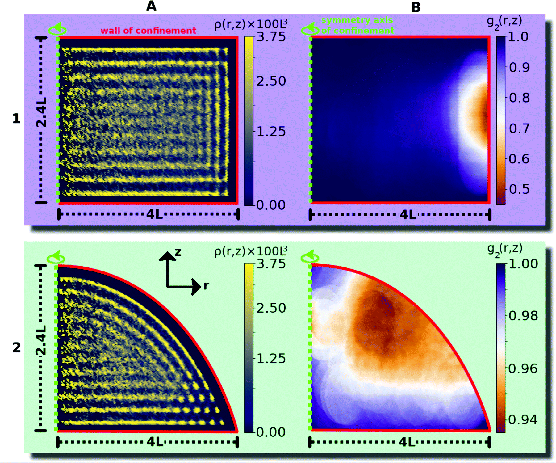
Previous studies on 2d smectics in a simply-connected convex confining cavity79,97,98 have shown the existence of a large, relatively defect-free central domain, encompassing several smectic layers, which connect opposite ends of the cavity. This bridge state can generally be observed for a large range of confinements.80 Indeed, we find that this reference structure also persists when extending the system into the third dimension.In our 3d study, we compare typical simulation results, shown both in Fig. 3 from a bird's eye view and in Fig. 4 using a 2d depiction, for two representative systems of hard rods confined to a cylindrical container (column 1) and spherical cap (column 2). The snapshots in Fig. 3A1 and A2 give an indication of the chosen dimensions of the confinement in terms of the dimensions of the individual particles: The height h of both cylinder and spherical cap is 2.4L, while the diameter 2R of the footprint is fixed at 8L. Both systems display what can be considered a generalized 3d bridge state. This becomes even clearer when considering the bottom view of both systems in Fig. 4A1 and A2. Apparently, the bottom layer of rods in our 3d systems forms 2d bridge states. Due to the symmetry of the cylinder, this structure is also mirrored on the top side. Even though the top surface of the spherical cap is strongly curved, the structure on it still resembles a 2d bridge state.
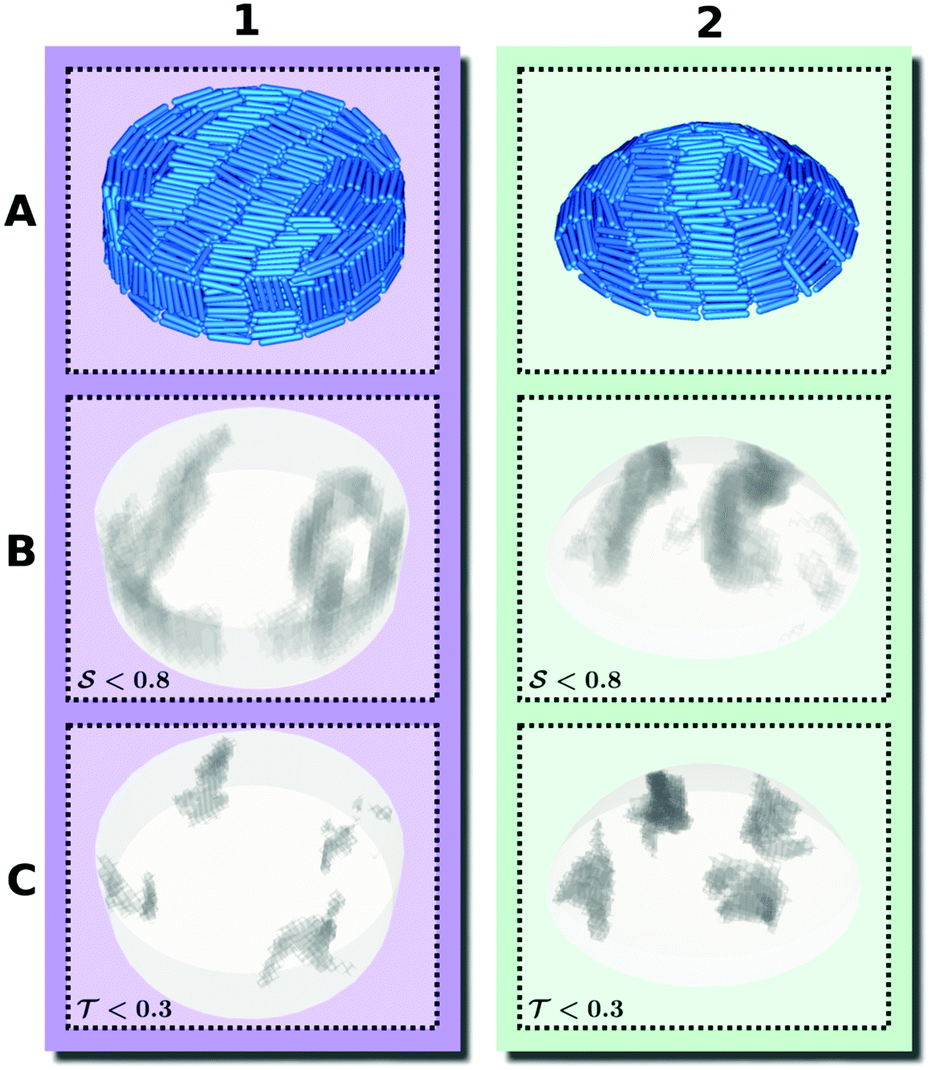 | ||
Fig. 3 Exemplary simulation results for two systems of 3d confined smectic liquid crystals. Column 1: cylinder. Column 2: spherical cap. Both systems feature height h = 2.4L and diameter 2R = 8L. Row A: Bird's eye view of the simulated system of hard rods. Row B: 3d visualization of the nematic defects according to the order parameter  . In order to observe the regions of low nematic order, i.e., defect regions, we display the data points with . In order to observe the regions of low nematic order, i.e., defect regions, we display the data points with  as opaque gray clouds. Row C: 3d visualization of the tetratic defects according to the 3d tetratic order parameter as opaque gray clouds. Row C: 3d visualization of the tetratic defects according to the 3d tetratic order parameter  . To visualize the defect regions, we only display the data points with . To visualize the defect regions, we only display the data points with  . . | ||
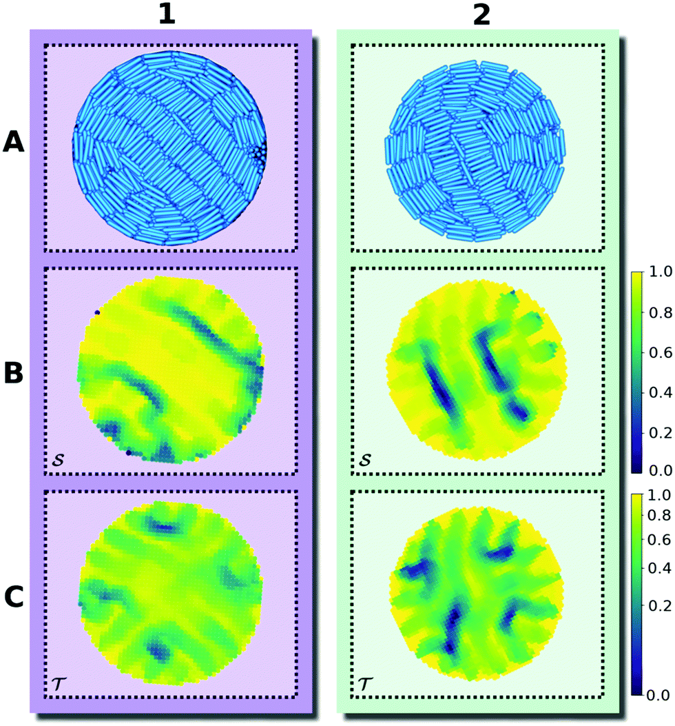 | ||
Fig. 4 The same two 3d systems as depicted in Fig. 3, but shown from a 2d perspective. Column 1: cylinder. Column 2: spherical cap. Row A: bottom view of the snapshots to exemplify the structure of the 2d cross-sections. Row B:  for the system projected onto the horizontal plane. Row C: for the system projected onto the horizontal plane. Row C:  for the system projected onto the horizontal plane. for the system projected onto the horizontal plane. | ||
To study the particle orientation throughout the system in more detail, we examine the topology of the corresponding order-parameter fields. In Fig. 3B1 and B2, we visualize the data points of low nematic order by showing the regions with  in gray. For both confinements, the resulting plots show a pair of planar disclinations, nestled to the sides of the central bridge domain. These defect planes reach from the top to the bottom of the container, while their shape barely varies along the vertical axis. Moreover, at cross sections of constant height, they have very little contact to the outer walls. This picture is reinforced in Fig. 4B1 and B2, which show the nematic field of the systems projected on the horizontal plane, i.e., the plane perpendicular to the symmetry axis. Indeed, these projections closely resemble the nematic field
  for 2d systems, confirming that the shape of the defect planes varies little along the vertical axis. In addition to these grain-boundary planes, the simulated cylindrical structure gives rise to several spots where
  is significantly decreased at the mantle surface. As can be seen in Fig. 3A1, these spots correspond to locations where layers of single-rod depth align with the cylinder mantle. For the spherical cap, the formation of such domains is largely suppressed by the curved boundary.
Fig. 3C1 and C2 similarly show regions of low 3d tetratic order according to the order parameter  . In analogy to the nematic case, we locate the defects by identifying the regions where this order is minimal. Due to the relatively high sensitivity to orientational fluctuations of
  , we display the data points only for
  in gray. It is then clearly visible that the nematic defect planes split into two tetratic defect pillars, each spanning from the bottom plane of the cavity to the top surface. Fig. 4C1 and C2 show the corresponding tetratic order-parameter field for the systems projected on the horizontal plane. This visualization shows that the minima in the order-parameter field are well localized and take an almost point-like shape. This again confirms that the tetratic disclinations in 3d appear as relatively straight lines, parallel to the vertical axis of the confinement.
In general, one identifies orientational defects as singular geometric objects in space, where the local director field (r) (see eqn (5)) jumps discontinuously. In particular, in 2d/3d liquid crystals with a smectic-A symmetry, the typical difference across any defect is π/2. As a result, nematic defects can be identified with the help of  . The same angular difference leads to a promotion of tetratic order everywhere except for the endpoints/edges, where the preferred orientation rotates. As a result, we identify a set of tetratic disclination points/lines, with the help of
  , that sit on the endpoints/edges of each nematic defect.
3.2 Confined smectic structure
To better understand the structural details of our confined smectics, we consider the number density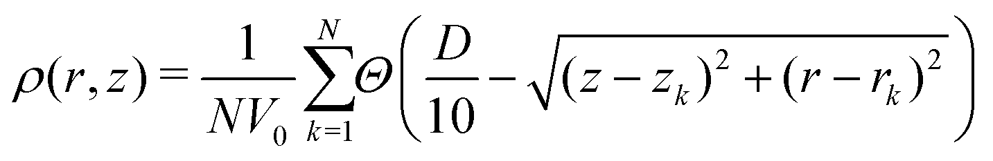 | (13) |
| g2(r, z) = 〈P2(sinθk)〉B2.5D(r,z), | (14) |
z), where sinθk denotes the orientation of the k-th particle projected into the horizontal plane and P2(x) is the second Legendre polynomial. To obtain an appropriate resolution, we average within a spherical subsystem of radius 2.5D.
Both quantities ρ(r,z) and g2(r,z) are averaged over 15 simulations runs, with different randomized initial states. We show the resulting distribution functions in Fig. 5 for the same confinements of container height h = 2.4L and diameter 2R = 8L, presented in Section 3.1. For ease of observation, the plots are stretched in the vertical direction. We generally observe for both confinements that the density profiles distinctly show the layering structure of the fluid, reflected by the relatively localized lines close to the outside walls. This indicates, that the positions of the layers are strongly influenced by the planar surface anchoring on the outer walls. While these peaks are less pronounced further inside the cavity, the diagrams show clear indication of horizontal stacking from the bottom to the top of the confinement. We stress that the kind of layering visible in the density profiles happens on the scale of the particle diameter D and should not be confused with smectic layering along the direction of the rod axes of length L + D.
 | ||
| Fig. 5 Averaged structural properties of smectic liquid crystals confined in a cylinder (row 1) and spherical cap (row 2) of height h = 2.4L and diameter 2R = 8L. All diagrams are shown in cylindrical coordinates, averaged over the azimuth around the vertical center axis of the confinement (shown as a dashed green line). All diagrams are additionally averaged over 15 simulations. Column A: one-particle density ρ(r, z) (defined by eqn (13)). These fields exemplify the layered fluid structure along a radial slice of the confinement, influenced by the planar surface anchoring of the confinement. To improve the contrast, we set the interval of the color bar to [0, 3.75], ensuring that the structures are clearly visible. All values above 3.75 are mapped to 3.75. Column B: correlation g2(r, z) (defined by eqn (14)) of the orientations at a certain position with the orientations projected into the horizontal plane. This function illustrates the deviation from the preferred horizontal orientation depending on the position within the confinement. | ||
Along the vertical axis, the density profile for cylindrical confinement in Fig. 5A1 shows 11 layers of particles within a length interval of 2.4L = 12D, indicating that their typical orientation is horizontal. This observation is reinforced in Fig. 5B1, showing that the orientations of the rods strongly correlate with the horizontal plane in almost the whole container. The depicted correlation function additionally indicates the presence of vertical rods close to the mantle of the cylinder, where g2(r, z) drops to g2 ≈ 0.3, consistent with the occasional appearance of vertical rods on the perimeter of the cylinder shown in the snapshot in Fig. 3A1. Accordingly, the density profile in Fig. 5A1 indicates a transition between vertical layers close to the mantle and horizontal layers in all other regions. In the corners, where the horizontal and vertical layers are compatible, we find fairly sharp isolated point-like peaks, exemplifying the high probability of a rod to sit aligned to both neighboring walls.
The density profile for the spherical-cap-shaped container in Fig. 5A2 indicates 12 stacked fluid layers in the middle of the confinement, indicating a stronger compression of the fluid than in the cylinder. Layers which are closer to the curved surface of the container are bent, while those closer to the bottom surface are horizontal. Again, we see localized peaks close to the corner, which are even more pronounced than in the cylindrical container due to the smaller opening angle. Here, the roughly 20 isolated peaks are arranged on an approximately hexagonal grid, representing the structure of rods sitting at an angle of π/2 to both walls, at approximately the same distances to the perimeter in all simulations. This clearly demonstrates the influence of the extreme confinement. Fig. 5B2 shows the orientational correlation of the rods g2 with the bottom plane. It is visible that all rods are aligned fairly horizontally within the whole spherical cap (mind the different color scale compared to the cylindrical cavity). Only in the vicinity of the curved surface of the container, g2(r, z) is slightly reduced to values of g2 ≈ 0.9, indicating that the rods rotate slightly out of the horizontal plane when aligning with the curved wall.
To study the effect of confinement height h in more detail, we vary this geometrical parameter from h = 0.3L to h = 4.5L in steps of 0.3L, performing in each case 15 simulations for each confining geometry. In Fig. 6, we show the resulting nematic order parameter  and the 3d tetratic order parameter
  evaluated for the entire system as a function of h. For the spherical cap, both order parameters
  and
and  globally remain at fairly constant values, irrespective of the confinement height h. In detail, the nematic order parameter settles at
  , while the tetratic order parameter settles at
  , only showing a slight downwards trend. In stark contrast, for cylindrical confinement the tetratic order parameter increases strongly with increasing h, while the nematic order parameter displays a nonmonotonic behavior.
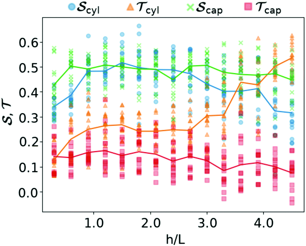 | ||
Fig. 6 Nematic order parameter  and tetratic order parameter and tetratic order parameter  (see Section 2.2) for the smectic liquid crystals confined to 3d cavities in the shape of cylinders and spherical caps (see Fig. 1). Along the horizontal axis we show a range of confinements with different heights h in units of spherocylinder length L. The vertical axis represents different values of the order parameters evaluated for the entire system. For each confinement, we performed 15 simulations for each value of h. The height h is swept from h = 0.3L up to h = 4.5L in steps of 0.3L. For each simulation run, we show two sets of data points, corresponding to the two order parameters (see Section 2.2) for the smectic liquid crystals confined to 3d cavities in the shape of cylinders and spherical caps (see Fig. 1). Along the horizontal axis we show a range of confinements with different heights h in units of spherocylinder length L. The vertical axis represents different values of the order parameters evaluated for the entire system. For each confinement, we performed 15 simulations for each value of h. The height h is swept from h = 0.3L up to h = 4.5L in steps of 0.3L. For each simulation run, we show two sets of data points, corresponding to the two order parameters  and and  . The curves show the order parameters averaged over the 15 simulation runs. . The curves show the order parameters averaged over the 15 simulation runs. | ||
Comparing the ordering behavior in the two types of cavities in more detail, we also observe in Fig. 6 that for the most shallow confinements with h = 0.3L the two values of  are qualitatively similar, whereas
  takes a slightly lower value in the cylinder than in the cap. For this small height of the cavities, there are practically no effects of the third dimension, such that, like in a true 2d system, the aspect ratio p = 5 of the rods considered here is too small to result in a significant orientational order and much less a smectic bridge state. The fact that the global nematic ordering in the spherical cap is still higher than in the cylinder, relates to the decreased accessible radius of the effective circular confinement. Upon departing from this quasi-2d case by increasing h, the global order generally increases. For the cylinder, however, the nematic order parameter decreases again from
  to
to  , while
  drastically increases from
  to
to  as soon as h > 1.5L. This behavior, which is specific for the cylindrical geometry, can be explained by the fact that we observe a higher fraction of vertical rods on the mantle surface for taller confinements, reducing the global nematic order. In turn, this alignment even leads to an increase of the tetratic order, since the vertical rods are perfectly perpendicular to the central domain, such that the tetratic defects, which are exclusively formed by the horizontal rods, take a smaller percentage of the total system size. This kind of behavior is not observed for the spherical cap due to its curved boundary. For even larger cylinder heights h, the majority of rods aligns with the mantle surface such that the global nematic order increases again. This is studied in detail in Appendix B.
3.3 Topological charge
In Section 3.1, we discussed the detection of the topological defects with the help of the order parameters. As elaborated in Section 2.3, topological defects that span between system boundaries, such as those in Fig. 3 and 4, can be assigned a topological charge defined via the net rotation of the director(r) along an encircling closed contour. More specifically, these contours can be defined within any cross section parallel to the bottom plane. Note that the sum of all topological charges, defined in this way, is a conserved quantity in 3d only under specific circumstances like in the smectic systems considered here, which can be understood as follows. Imagine, e.g., that Fig. 2A1 and A2 represent cross sections of a 3d nematic system (rather than a purely 2d system). In this case, the Q = +1/2 defect from Fig. 2A1 can be transformed into the Q = −1/2 defect from Fig. 2A2 by flipping the orientations ûk of all rods individually across the vertical picture axis. This transformation can be performed as a continuous mapping in 3d space, thereby obtaining a Q = +1/2 defect from a Q = −1/2 or vice versa. Additionally, this rotation can occur continuously along a disclination line, resulting in different values for topological charges, depending on the respective chosen cross section.81 As a result, all possible structures can in principle be either homotopically equivalent to a charge-free structure with Q = 0 or to a defect structure with Q = 1/2.
In the previous Section 3.2, we elaborated that the confined smectic fluids in our simulations majorly consist of stacked quasi-2d layers. By showing that the 3d systems consist of a number of stacked quasi-2d layers, with no out-of-plane rotation, the defects do not undergo the transitions mentioned above. We thus argue that, in our simulations, the topological charge is equal for all horizontal cross sections, such that we can consistently define charges of any of the defects visible in Fig. 3. Additionally, we observe very similar structures on the top and bottom surface of the cylindrical systems and even on the curved surface of the spherical cap. This similarity of top and bottom structures is a further indication for a persisting structure through all horizontal slices. We can thus assume, to a good degree of approximation, that the director (r) does not rotate out of the 2d layers the 3d system consists of. This reduces the orientational configuration space from S2/Z2 to S1/Z2, implying that we can treat the topology in full analogy to the 2d case. In this way, by observing the bottom plane, we can infer that the total topological charge of the nematic grain boundary is equal to Q = 1/2 and matches the charge of the 2d counterpart. More specifically, the grain boundaries split into two pillars, i.e., tetratic disclination lines, with q = 1/4 each, corresponding to q = 1/4 point charges in the cross-sections.
Less frequent exceptions to the ordering behavior described above for the considered confinements are given by the occasional alignment of the rods with the curved surface of the cap-shaped container as well as the small vertical clusters present at the mantle surface of the cylindrical container. The former case does not undergo a transition between ±1/2 charged cross sections, as no rods are present that are drastically rotated out of plane. This is supported by the fact that the flat projection of the structure on the curved surface still mirrors the structure of the bottom plane. For cylindrical cavities of comparable height, according to our observation, a director field (r) can most of the time be defined in a neighborhood around the defect, such that the vertical clusters do not influence the topological charges. This is in general no longer the case when the cylinder becomes sufficiently tall. As shown in Appendix B, for h ≳ 5L full layers of vertical rods persist throughout several cross sections.
From mathematical topology it follows that for liquid crystals confined to 2d manifolds, the total topological charge in the director field has to match the Euler characteristic χ of the container.91 The Euler characteristic χ is an algebraic invariant. Accordingly, results of previous work agree for nematic59 as well as smectic liquid crystals80 confined to simply-connected convex cavities and for smectics confined to 2d spherical surfaces embedded in 3d.60 In this work, we have presented examples for 3d simply-connected convex confinements, where the sum of topological charges defined through integrating around a closed contour in a 2d cross section matches the Euler characteristic χ = 1 of this cross section.
4 Conclusion
In this work, we provided an insight into the topology of defects in 3d smectic liquid crystals. In 3d smectic liquid crystals, orientational defects take the shape of extended planar grain boundaries, across which the local preferred direction jumps by an angle of π/2. Combining the established knowledge of classification of 3d nematic disclination lines with recent insights into the classification of grain boundaries as orientational defects in 2d smectic liquid crystals, we presented a formalism for the analysis of topological charge distribution. We exemplified this formalism on smectic structures in cylindrical and spherical cap containers, obtained using Monte-Carlo simulation.In the 2d analysis one can utilize the coexistence of nematic and tetratic defects and, with the help of the tetratic order parameter, locate the points where the preferred direction rotates. Accordingly, we introduced a tetratic order parameter which can be readily applied to 3d systems. The 3d tetratic line defects were then analyzed along 2d cross sections.
In a 3d system, the sum of the winding numbers of all defects is not in general a conserved quantity since defects with different winding numbers can be transformed into each other. However, since the confined structures can be interpreted as stacked quasi-2d systems, topological charge behaves akin to electromagnetic charge and follows similar additive conservation laws. We thus found in the simulated systems that the total topological charge matches the Euler characteristic χ = 1 of the containers and splits into two orientational defects, i.e., two grain boundaries with topological charge Q = 1/2 each. Those can in turn be split into two tetratic disclination lines with charges q = 1/4. In general terms, we find it remarkable that the 2d topological charge, which does not have to be conserved for mathematical reasons in three dimensions, is conserved for physical reasons in the systems considered in this work.
To better understand the physical origin of the pronounced grain boundaries emerging in our confined system, let us recall that a key property of the (hard-core) colloidal system under consideration is the rigidity of the smectic layers, such that the balance between intrinsic structure and external constraints mostly results in extended defects (grain boundaries) rather than elastic deformations. A similar observation has been made for a related 2d system using both microscopic density functional theory and colloidal experiments79 and we expect that the same mechanism is at work in three dimensions. To get further insight, the confined systems considered in this work could therefore be investigated using density functionals for hard spherocylinders.99,100 Alternatively, density functional theory also allows to determine elastic parameters of fluids of hard spherocylinders101 which could then be used to fix the parameters in phenomenological elasticity theories100,102,103 for the smectic phase.
Throughout this paper, we have in particular shed light on planar grain boundaries which split into two tetratic disclination lines. Our insight will thus be useful for the interpretation of future computational,104,105 theoretical,99–104,106 and experimental79,98,107–109 research on confined smectic structures in three dimensions. To this end, our topological picture can be extended to study more complex geometries and topologies in 3d, e.g., by observing q = −1/4 tetratic defects, which, in analogy to the 2d case, should emerge at junction points of defect networks in confinements that promote multiple domains80 or close to concave regions of the system boundary.79 Of interest may also be the investigation of the connection of orientational defects to positional defects, such as dislocations and focal conic domains. In nematic systems, it is widely accepted that the dynamical properties of a defect are influenced by the respective topological charge.1,20,66–68,110 Therefore, understanding the role of smectic orientational defects, i.e., grain boundaries analyzed as a connected pair of tetratic defects, in nonequilibrium is also of particular importance for understanding, e.g., nucleation processes111–114 and the dynamics115 of smectics, as well as active liquid crystal systems,18–21 which might also exhibit smectic order.
Conflicts of interest
There are no conflicts to declare.Appendix A: tetratic order parameter in three dimensions
In this appendix, we provide an appropriate definition of the tetratic order parameter to characterize the topological fine structure in smectic systems of uniaxial rods.1. Definition
In general, a system of N uniaxial particles can be microscopically described by a distribution function f(û) that reads | (A1) |
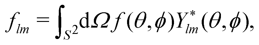
θcosϕ, sinθsinϕ, cosθ)T is the orientation vector. Such a function can be expanded as116 | (A2) |
 | (A3) |
 . An expansion of the form (A2) is also possible in a 2d system, in this case û is a 2d vector depending on just one angle and the expression (A3) is slightly modified (see ref. 116). The second-order contribution
  is the nematic tensor. (In the main text (eqn (5)), we have, as is common, defined it with a different normalization that corresponds to multiplying the one resulting from eqn (A3) by 4π/5.) An interesting mathematical property of the Cartesian expansion (A2) is that it is orderwise equivalent to the spherical multipole expansion
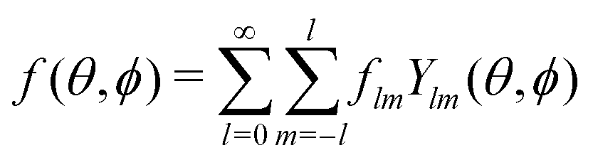 | (A4) |
 | (A5) |
We are now looking for an order parameter that identifies configurations as ordered if the rods are either parallel or orthogonal to each other. In the 2d case, this can be simply done by superimposing tetratic order,80i.e., fourfold rotational symmetry. Mathematically, this corresponds to measuring defects not in the nematic order-parameter field, corresponding to the second-order term in the 2d version of eqn (A2), but in the fourth-order contribution. This suggests that the desired order parameter can be constructed from the fourth-order term (l = 4) in eqn (A2) also in the 3d case. Since the Cartesian order parameter at fourth order has 81 components of which, due to symmetry and tracelessness, only 9 are independent, it is more convenient to work with the expansion coefficients of the angular expansion (A4) instead.
From eqn (A1) and (A5) we would then get the order parameters
 | (A6) |
 | (A7) |
Finally, we also need to take into account that the order parameter constructed from the invariants Il should (a) be normalized – this can simply be ensured by multiplying it by an appropriate prefactor – and (b) not distinguish between parallel and orthogonal rods. Unfortunately, the invariant I4 gives a larger value for parallel than for orthogonal configurations. To correct for this, we exploit the fact that the invariant I2 measures nematic order,120,121 such that it is large for parallel configurations. Hence, our generalized order parameter should be proportional to I4 − βI2, where β is a suitable prefactor. We have found an appropriate choice to be β = 3/4. Thus, we arrive at the tetratic order parameter
 | (A8) |
 is always positive. We have tested a range of possible configurations and found that I4 − βI2 < 0 is measured only for isotropic systems with |I4 − βI2| ≪ 1 (probably due to numerical fluctuations). This is reinforced by the notion that I2 measures nematic order and systems with high nematic order result in
  ≈ 1.
≈ 1.
5.2 Examples
To get an exemplary system that should be perfectly ordered by our definition, consider three orthogonal particles with orientations (θ1, ϕ1) = (π/2, 0), (θ2, ϕ2) = (π, 0) and (θ3, ϕ3) = (π/2, π/2). We find | (A9) |
 | (A10) |
 | (A11) |
Appendix B: taller cylinders
The height h of a spherical cap is limited by the full sphere with h = 2R, but the respective height of a cylindrical cavity can, in principle, be chosen arbitrarily large. While in the main text, we focus on heights of the cylinder which are also possible in the cap geometry, we discuss in this appendix the behavior of the same liquid crystal systems confined to taller cylinders up to a height h = 15L (i.e., up to N ≈ 1.1 × 10⁴ particles). Our results are shown in Fig. 7. | ||
Fig. 7 Properties of smectic liquid crystals confined to cylinders of diameter 2R = 8L as shown in the main text but with taller heights h. (A) Representative snapshot for h = 14L from a bird's eye view, as in Fig. 3A1. The picture below shows the bottom side of the same system, from the same azimuthal viewing angle. (B) Correlation function g2(r, z) (defined by eqn (14)) of the orientations at a certain position with the orientations projected into the horizontal plane for h = 14L, as in Fig. 5. Here, the field is generated as average over five simulation runs. (C) Nematic and tetratic order parameters  and and  (see Section 2.2) with additional data for h ∈ [5L, 15L], taken from five simulation runs. The gray background indicates the interval h ∈ [0.3L, 4.5L] which includes the data from Fig. 6. (see Section 2.2) with additional data for h ∈ [5L, 15L], taken from five simulation runs. The gray background indicates the interval h ∈ [0.3L, 4.5L] which includes the data from Fig. 6. | ||
The snapshot in Fig. 7A depicts a system in a cylinder of height h = 14L. It is clearly visible that, along the entire mantle surface, the rods are aligned with the main axis of the cylinder. The structure at both the top and bottom layer in the cylinder (visible in the upper and lower picture, respectively, shown from the same, azimuthal viewing angle) still resembles a bridge state, which for the shorter cylindrical cavities was found to persist throughout the whole system. However, the two bridging domains have a different in-plane orientation, indicating that the structures at the top and bottom are independent.
Fig. 7B shows the orientational distribution g2(r, z) (defined by eqn (14)) sampled as average over five simulation snapshots from systems with h = 14L. Here, the independence of the two horizontal layers of rods at the top and bottom of the cavity becomes apparent, since throughout the majority of the system the rods are vertical. More specifically, contrasting this observation to Fig. 5B1, we notice that here the signal indicating a vertical orientation percolates throughout several horizontal slices, while for shorter cylinders the signal indicating the horizontal orientation percolates from top to bottom. Taking a closer look at the distribution for the tall cylinder, we observe that the vertical regime is slightly perturbed by horizontal stripes in the field at a distance corresponding to the smectic layer spacing. These dips correspond to the occasional occurrence of horizontal rods between the layers,122 as is also visible in the snapshot in Fig. 7A.
Fig. 7C shows the 3d tetratic order parameter  as well as the standard nematic order parameter
  (see Section 2.2) for a range h ∈ [0.3L, 15L] of cylinder heights as an extension of Fig. 6. As the behavior for extremely shallow cavities has been discussed in detail in Section 3.2, we focus here on larger values of h. It is clearly visible from Fig. 7C that
  has a minimum at h ≈ 5L, which reflects the transition from a structure with the majority of rods aligning horizontally along the top and bottom plates for short cylinders to a structure with the majority of rods aligning vertically along the cylinder mantle for tall cylinders. In the latter case, two additional grain boundaries between horizontal and vertical rods emerge close to the two ends of the cylinder, decreasing the global nematic order. When further increasing h ≳ 5L, the nematic order parameter
  increases again until eventually reaching a plateau when the fraction of the horizontal rods and the corresponding defects become negligible. In stark contrast, the value of the tetratic order parameter
  is not affected by the relative size of the interface between horizontal and vertical domains, such that there is no minimum around h ≈ 5L. Instead, as soon as the vertical rods become relevant,
  increases monotonously with increasing cylinder height h and plateaus already at h ≈ 6L, since the tetratic defects (cf.Fig. 3C1) are only located in the horizontal layers.
Acknowledgements
We thank Arjun Yodh and Alice Rolf for helpful discussions. This work is funded by the Deutsche Forschungsgemeinschaft (DFG, German Research Foundation) – VO 899/19-2; WI 4170/3-1; LO 418/20-2. M. t. V. thanks the Studienstiftung des deutschen Volkes for financial support.References
- N. D. Mermin, Rev. Mod. Phys., 1979, 51, 591 CrossRef CAS.
- T. W.-B. Kibble, J. Phys. A, 1976, 9, 1387 CrossRef.
- T. Shinjo, T. Okuno, R. Hassdorf, K. Shigeto and T. Ono, Science, 2000, 289, 930 CrossRef PubMed.
- C. Phatak, A. K. Petford-Long and O. Heinonen, Phys. Rev. Lett., 2012, 108, 067205 CrossRef CAS PubMed.
- L. Lu, J. D. Joannopoulos and M. Soljačić, Nat. Photonics, 2014, 8, 821 CrossRef CAS.
- A. Moor, A. F. Volkov and K. B. Efetov, Phys. Rev. B, 2014, 90, 224512 CrossRef.
- A. Tan, J. Li, A. Scholl, E. Arenholz, A. T. Young, Q. Li, C. Hwang and Z. Q. Qiu, Phys. Rev. B, 2016, 94, 014433 CrossRef.
- G. Yi and B. D. Youn, Struct. Multidiscip. Optim., 2016, 54, 1315 CrossRef.
- A. O. Sorokin, Phys. Rev. B, 2017, 95, 094408 CrossRef.
- Y. Liu, Z. Wang, T. Sato, M. Hohenadler, C. Wang, W. Guo and F. F. Assaad, Nat. Commun., 2019, 10, 2658 CrossRef PubMed.
- X. Lu, R. Fei, L. Zhu and L. Yang, Nat. Commun., 2020, 11, 4724 CrossRef PubMed.
- C. Wang, C.-H. Chang, A. Herklotz, C. Chen, F. Ganss, U. Kentsch, D. Chen, X. Gao, Y.-J. Zeng and O. Hellwig, et al. , Adv. Electron. Mater., 2020, 6, 2000184 CrossRef CAS.
- P.-G. De Gennes and J. Prost, The physics of liquid crystals, Oxford University Press, Oxford, UK, 1993 Search PubMed.
- M. C. Marchetti, J.-F. Joanny, S. Ramaswamy, T. B. Liverpool, J. Prost, M. Rao and R. A. Simha, Rev. Mod. Phys., 2013, 85, 1143 CrossRef CAS.
- C. E. Fowler, W. Shenton, G. Stubbs and S. Mann, Adv. Mater., 2001, 13, 1266 CrossRef CAS.
- Z. Reich, E. J. Wachtel and A. Minsky, Science, 1994, 264, 1460 CrossRef CAS PubMed.
- I. W. Hamley, Soft Matter, 2010, 6, 1863 RSC.
- L. Giomi, Phys. Rev. X, 2015, 5, 031003 Search PubMed.
- S. J. DeCamp, G. S. Redner, A. Baskaran, M. F. Hagan and Z. Dogic, Nat. Mater., 2015, 14, 1110 CrossRef CAS PubMed.
- A. J. Tan, E. Roberts, S. A. Smith, U. A. Olvera, J. Arteaga, S. Fortini, K. A. Mitchell and L. S. Hirst, Nat. Phys., 2019, 15, 1033 Search PubMed.
- S. Shankar, A. Souslov, M. J. Bowick, M. C. Marchetti and V. Vitelli, 2020, arXiv:2010.00364.
- K. Beppu, Z. Izri, J. Gohya, K. Eto, M. Ichikawa and Y. T. Maeda, Soft Matter, 2017, 13, 5038 RSC.
- A. Sokolov, I. S. Aranson, J. O. Kessler and R. E. Goldstein, Phys. Rev. Lett., 2007, 98, 158102 CrossRef PubMed.
- H. H. Wensink, J. Dunkel, S. Heidenreich, K. Drescher, R. E. Goldstein, H. Löwen and J. M. Yeomans, Proc. Natl. Acad. Sci. U. S. A., 2012, 109, 14308 CrossRef CAS PubMed.
- J. Dunkel, S. Heidenreich, K. Drescher, H. H. Wensink, M. Bär and R. E. Goldstein, Phys. Rev. Lett., 2013, 110, 228102 CrossRef PubMed.
- F. J. Ndlec, T. Surrey, A. C. Maggs and S. Leibler, Nature, 1997, 389, 305 CrossRef PubMed.
- V. Schaller, C. Weber, C. Semmrich, E. Frey and A. R. Bausch, Nature, 2010, 467, 73 CrossRef CAS PubMed.
- S. J. Hall, C. S. Wardle and D. N. MacLennan, Mar. Biol., 1986, 91, 143 CrossRef.
- N. Abaid and M. Porfiri, J. R. Soc., Interface, 2010, 7, 1441 CrossRef PubMed.
- M. Dijkstra, R. van Roij and R. Evans, Phys. Rev. E, 2001, 63, 051703 CrossRef CAS PubMed.
- P. E. Brumby, H. H. Wensink, A. J. Haslam and G. Jackson, Langmuir, 2017, 33, 11754 CrossRef CAS PubMed.
- E. Basurto, P. Gurin, S. Varga and G. Odriozola, Phys. Rev. Res., 2020, 2, 013356 CrossRef CAS.
- C. Chiccoli, P. Pasini, F. Semeria and C. Zannoni, Mol. Cryst. Liq. Cryst., 1992, 221, 19 CrossRef.
- O. D. Lavrentovich, Liq. Cryst., 1998, 24, 117 CrossRef CAS.
- Y.-K. Kim, S. V. Shiyanovskii and O. D. Lavrentovich, J. Condens. Matter Phys., 2013, 25, 404202 CrossRef PubMed.
- P. Prinsen and P. van der Schoot, Phys. Rev. E, 2003, 68, 021701 CrossRef PubMed.
- Y. Trukhina, S. Jungblut, P. van der Schoot and T. Schilling, J. Chem. Phys., 2009, 130, 164513 CrossRef PubMed.
- Y. Trukhina and T. Schilling, Phys. Rev. E, 2008, 77, 011701 CrossRef PubMed.
- D. de las Heras, E. Velasco and L. Mederos, Phys. Rev. E, 2009, 79, 061703 CrossRef CAS PubMed.
- O. J. Dammone, I. Zacharoudiou, R. P.-A. Dullens, J. M. Yeomans, M. P. Lettinga and D. G.-A. L. Aarts, Phys. Rev. Lett., 2012, 109, 108303 CrossRef PubMed.
- O. V. Manyuhina, K. B. Lawlor, M. C. Marchetti and M. J. Bowick, Soft Matter, 2015, 11, 6099 RSC.
- A. Majumdar and A. Lewis, Liq. Cryst., 2016, 43, 2332 CrossRef CAS.
- A. H. Lewis, I. Garlea, J. Alvarado, O. J. Dammone, P. D. Howell, A. Majumdar, B. M. Mulder, M. Lettinga, G. H. Koenderink and D. G.-A. L. Aarts, Soft Matter, 2014, 10, 7865 RSC.
- I. C. Gârlea, P. Mulder, J. Alvarado, O. J. Dammone, D. G.-A. L. Aarts, M. P. Lettinga, G. H. Koenderink and B. M. Mulder, Nat. Commun., 2016, 7, 12112 CrossRef PubMed.
- A. Daz-De Armas, M. Maza-Cuello, Y. Martnez-Ratón and E. Velasco, Phys. Rev. Res., 2020, 2, 033436 CrossRef.
- X. Yao and J. Z.-Y. Chen, Phys. Rev. E, 2020, 101, 062706 CrossRef CAS PubMed.
- X. Yao, H. Zhang and J. Z.-Y. Chen, Phys. Rev. E, 2018, 97, 052707 CrossRef PubMed.
- X. Yao, L. Zhang and J. Z.-Y. Chen, Phys. Rev. E, 2022, 105, 044704 CrossRef.
- P. Poulin, V. Cabuil and D. A. Weitz, Phys. Rev. Lett., 1997, 79, 4862 CrossRef CAS.
- R. W. Ruhwandl and E. M. Terentjev, Phys. Rev. E, 1997, 56, 5561 CrossRef CAS.
- D. Andrienko, G. Germano and M. P. Allen, Phys. Rev. E, 2001, 63, 041701 CrossRef CAS PubMed.
- H. Stark, Phys. Rep., 2001, 351, 387 CrossRef CAS.
- S. Čopar, T. Porenta, V. S.-R. Jampani, I. Muševič and S. Žumer, Soft Matter, 2012, 8, 8595 RSC.
- J. M. Ilnytskyi, A. Trokhymchuk and M. Schoen, J. Chem. Phys., 2014, 141, 114903 CrossRef PubMed.
- S. Püschel-Schlotthauer, V. Meiwes Turrión, C. K. Hall, M. G. Mazza and M. Schoen, Langmuir, 2017, 33, 2222 CrossRef PubMed.
- K. Chen, O. J. Gebhardt, R. Devendra, G. Drazer, R. D. Kamien, D. H. Reich and R. L. Leheny, Soft Matter, 2018, 14, 83 RSC.
- K. H. Kil, A. Yethiraj and J. S. Kim, Phys. Rev. E, 2020, 101, 032705 CrossRef CAS PubMed.
- B. Loewe and T. N. Shendruk, New J. Phys., 2022, 24, 012001 CrossRef.
- J. Dzubiella, M. Schmidt and H. Löwen, Phys. Rev. E, 2000, 62, 5081 CrossRef CAS PubMed.
- E. Allahyarov, A. Voigt and H. Löwen, Soft Matter, 2017, 13, 8120 RSC.
- F. C. Keber, E. Loiseau, T. Sanchez, S. J. DeCamp, L. Giomi, M. J. Bowick, M. C. Marchetti, Z. Dogic and A. R. Bausch, Science, 2014, 345, 1135 CrossRef CAS PubMed.
- S. Kralj, R. Rosso and E. G. Virga, Soft Matter, 2011, 7, 670 RSC.
- I. Nitschke, M. Nestler, S. Praetorius, H. Löwen and A. Voigt, Proc. R. Soc. A, 2018, 474, 20170686 CrossRef PubMed.
- M. Nestler, I. Nitschke, H. Löwen and A. Voigt, Soft Matter, 2020, 16, 4032 RSC.
- I. Nitschke, S. Reuther and A. Voigt, Proc. R. Soc. A, 2020, 476, 20200313 CrossRef PubMed.
- A. J. Vromans and L. Giomi, Soft Matter, 2016, 12, 6490 RSC.
- K. Harth and R. Stannarius, Front. Phys., 2020, 8, 112 CrossRef.
- G. Tóth, C. Denniston and J. M. Yeomans, Phys. Rev. Lett., 2002, 88, 105504 CrossRef PubMed.
- G. P. Alexander, B. G.-g Chen, E. A. Matsumoto and R. D. Kamien, Rev. Mod. Phys., 2012, 84, 497 CrossRef CAS.
- M. Kléman, Rep. Prog. Phys., 1989, 52, 555 CrossRef.
- R. B. Meyer, B. Stebler and S. T. Lagerwall, Phys. Rev. Lett., 1978, 41, 1393 CrossRef CAS.
- P. Chen and C.-Y. D. Lu, J. Phys. Soc. Jpn., 2011, 80, 094802 CrossRef.
- C. Zhang, A. M. Grubb, A. J. Seed, P. Sampson, A. Jákli and O. D. Lavrentovich, Phys. Rev. Lett., 2015, 115, 087801 CrossRef CAS PubMed.
- R. D. Kamien and R. A. Mosna, New J. Phys., 2016, 18, 053012 CrossRef.
- J. P. Bramble, S. D. Evans, J. R. Henderson, T. J. Atherton and N. J. Smith, Liq. Cryst., 2007, 34, 1137 CrossRef CAS.
- Y. H. Kim, D. K. Yoon, M.-C. Choi, H. S. Jeong, M. W. Kim, O. D. Lavrentovich and H.-T. Jung, Langmuir, 2009, 25, 1685 CrossRef CAS PubMed.
- D. B. Liarte, M. Bierbaum, R. A. Mosna, R. D. Kamien and J. P. Sethna, Phys. Rev. Lett., 2016, 116, 147802 CrossRef PubMed.
- M. Kléman and O. D. Lavrentovich, Eur. Phys. J. E, 2000, 2, 47 CrossRef.
- R. Wittmann, L. B.-G. Cortes, H. Löwen and D. G.-A. L. Aarts, Nat. Commun., 2021, 12, 623 CrossRef CAS PubMed.
- P. A. Monderkamp, R. Wittmann, L. B.-G. Cortes, D. G.-A. L. Aarts, F. Smallenburg and H. Löwen, Phys. Rev. Lett., 2021, 127, 198001 CrossRef CAS PubMed.
- S. Afghah, R. L.-B. Selinger and J. V. Selinger, Liq. Cryst., 2018, 45, 2022 CrossRef CAS.
- C. Vega and S. Lago, Comput. Chem., 1994, 18, 55 CrossRef CAS.
- H. C. Andersen, D. Chandler and J. D. Weeks, J. Chem. Phys., 1972, 56, 3812 CrossRef CAS.
- N. Metropolis, A. W. Rosenbluth, M. N. Rosenbluth, A. H. Teller and E. Teller, J. Chem. Phys., 1953, 21, 1087 CrossRef CAS.
- M. Kleman and O. D. Lavrentovich, Soft Matter Physics – An Introduction, Springer, New York, NY, 2003 Search PubMed.
- M. A. Bates and D. Frenkel, J. Chem. Phys., 2000, 112, 10034 CrossRef CAS.
- K. Zhao, C. Harrison, D. Huse, W. B. Russel and P. M. Chaikin, Phys. Rev. E, 2007, 76, 040401 CrossRef PubMed.
- P. J. Steinhardt, D. R. Nelson and M. Ronchetti, Phys. Rev. B, 1983, 28, 784 CrossRef CAS.
- J. A.-C. Veerman and D. Frenkel, Phys. Rev. A, 1992, 45, 5632 CrossRef PubMed.
- P. D. Duncan, M. Dennison, A. J. Masters and M. R. Wilson, Phys. Rev. E, 2009, 79, 031702 CrossRef PubMed.
- M. J. Bowick and L. Giomi, Adv. Phys., 2009, 58, 449 CrossRef CAS.
- F. C. Frank, Discuss. Faraday Soc., 1958, 25, 19 RSC.
- B. G.-g Chen, G. P. Alexander and R. D. Kamien, Proc. Natl. Acad. Sci. U. S. A., 2009, 106, 15577 CrossRef CAS PubMed.
- T. Machon, H. Aharoni, Y. Hu and R. D. Kamien, Commun. Math. Phys., 2019, 372, 525 CrossRef.
- R. Pindak, C. Y. Young, R. B. Meyer and N. A. Clark, Phys. Rev. Lett., 1980, 45, 1193 CrossRef CAS.
- H.-R. Trebin, Adv. Phys., 1982, 31, 195 CrossRef CAS.
- T. Geigenfeind, S. Rosenzweig, M. Schmidt and D. de las Heras, J. Chem. Phys., 2015, 142, 174701 CrossRef PubMed.
- L. B.-G. Cortes, Y. Gao, R. P.-A. Dullens and D. G.-A. L. Aarts, J. Phys.: Condens. Matter, 2017, 29, 064003 CrossRef PubMed.
- R. Wittmann, M. Marechal and K. Mecke, J. Chem. Phys., 2014, 141, 064103 CrossRef PubMed.
- R. Wittmann, M. Marechal and K. Mecke, J. Phys.: Condens. Matter, 2016, 28, 244003 CrossRef PubMed.
- R. Wittmann, M. Marechal and K. Mecke, Phys. Rev. E, 2015, 91, 052501 CrossRef PubMed.
- J. Xia, S. MacLachlan, T. J. Atherton and P. E. Farrell, Phys. Rev. Lett., 2021, 126, 177801 CrossRef CAS PubMed.
- J. Paget, M. G. Mazza, A. J. Archer and T. N. Shendruk, 2022, arXiv:2201.09019.
- M. Marechal, S. Dussi and M. Dijkstra, J. Chem. Phys., 2017, 146, 124905 CrossRef PubMed.
- M. Chiappini, E. Grelet and M. Dijkstra, Phys. Rev. Lett., 2020, 124, 087801 CrossRef CAS PubMed.
- D. de las Heras, E. Velasco and L. Mederos, Phys. Rev. E, 2006, 74, 011709 CrossRef CAS PubMed.
- W. Wang, G. Lieser and G. Wegner, Liq. Cryst., 1993, 15, 1 CrossRef CAS.
- T. Lopez-Leon, A. Fernandez-Nieves, M. Nobili and C. Blanc, J. Phys.: Condens. Matter, 2012, 24, 284122 CrossRef PubMed.
- A. Repula and E. Grelet, Phys. Rev. Lett., 2018, 121, 097801 CrossRef CAS PubMed.
- G. P. Crawford and S. Zumer, Liquid crystals in complex geometries: formed by polymer and porous networks, CRC Press, Boca Raton, Florida, USA, 1996 Search PubMed.
- H. Maeda and Y. Maeda, Phys. Rev. Lett., 2003, 90, 018303 CrossRef PubMed.
- T. Schilling and D. Frenkel, Phys. Rev. Lett., 2004, 92, 085505 CrossRef PubMed.
- R. Ni, S. Belli, R. van Roij and M. Dijkstra, Phys. Rev. Lett., 2010, 105, 088302 CrossRef PubMed.
- A. Cuetos, E. Sanz and M. Dijkstra, Faraday Discuss., 2010, 144, 253 RSC.
- E. Grelet, M. P. Lettinga, M. Bier, R. van Roij and P. van der Schoot, J. Phys.: Condens. Matter, 2008, 20, 494213 CrossRef.
- M. te Vrugt and R. Wittkowski, AIP Adv., 2020, 10, 035106 CrossRef.
- M. te Vrugt and R. Wittkowski, Ann. Phys., 2020, 532, 2000266 CrossRef.
- W. Lechner and C. Dellago, J. Chem. Phys., 2008, 129, 114707 CrossRef PubMed.
- H. Tanaka, Eur. Phys. J. E, 2012, 35, 113 CrossRef PubMed.
- B. S. John, C. Juhlin and F. A. Escobedo, J. Chem. Phys., 2008, 128, 044909 CrossRef PubMed.
- R. Blaak, D. Frenkel and B. M. Mulder, J. Chem. Phys., 1999, 110, 11652 CrossRef CAS.
- R. van Roij, P. Bolhuis, B. Mulder and D. Frenkel, Phys. Rev. E, 1995, 52, R1277 CrossRef CAS PubMed.
| This journal is © the Owner Societies 2022 |