Simulating core electron binding energies of halogenated species adsorbed on ice surfaces and in solution via relativistic quantum embedding calculations

Abstract

In this work, we investigate the effects of the environment on the X-ray photoelectron spectra of hydrogen chloride and chloride ions adsorbed on ice surfaces, as well as of chloride ions in water droplets. In our approach, we combine a density functional theory (DFT) description of the ice surface with that of halogen species using the recently developed relativistic core–valence separation equation of motion coupled cluster (CVS-EOM-IP-CCSD) via the frozen density embedding formalism (FDE), to determine the K and L_1,2,3 edges of chlorine. Our calculations, which incorporate temperature effects through snapshots from classical molecular dynamics simulations, are shown to reproduce experimental trends in the change of the core binding energies of Cl⁻ upon moving from a liquid (water droplets) to an interfacial (ice quasi-liquid layer) environment. Our simulations yield water valence band binding energies in good agreement with experiment, which vary little between the droplets and the ice surface. For halide core binding energies there is an overall trend for overestimating experimental values, though good agreement between theory and experiment is found for Cl⁻ in water droplets and on ice. For HCl on the other hand there are significant discrepancies between experimental and calculated core binding energies when we consider structural models that maintain the H–Cl bond more or less intact. An analysis of models that allow for pre-dissociated and dissociated structures suggests that experimentally observed chemical shifts in binding energies between Cl⁻ and HCl would require that H⁺ (in the form of H₃O⁺) and Cl⁻ are separated by roughly 4–6 Å.

---

1 Introduction

Ice is everywhere in the environment and its peculiar structure and properties make it a subject of intense scientific research. Studies connected to ice indicate that it hosts reactions that can influence climate, air quality, and biology systems and initiate ozone destruction.^1–3 Hydrogen bonding (HB) between ice and trace gases is the first step towards their interaction.⁴ Investigations into the bound state of the interaction of strong acids⁵ with ice indicate that strong acids lead to modification in the HB network of a liquid-like layer on the ice surface. It has been shown however that weak acid adsorption on the ice surface does not produce any significant changes in the HB network of water ice.⁶

In this respect, the influence of strong acids, in particular, hydrogen chloride (HCl) and its dissociated ionic chloride by ice, has attracted a lot of attention over the years due to their link to ozone depletion.⁷

A better understanding of the chemical processes associated with how the reactions of these reservoir gases on the ice surface differ from that of the bulk ice surface is essential for their interpretation and consequently for atmospheric science and environmental chemistry. Surface-specific spectroscopic approaches have been instrumental in gathering detailed information on the structural and electronic properties of solvated halide/halide ions,^8,9 and among these X-ray Photoelectron Spectroscopy (XPS) emerge as a particularly powerful technique¹⁰ due to its high specificity and the great sensitivity of core binding energies (BEs) to small perturbations to the surroundings of the atoms of interest.^11–15

The surface sensitivity and chemical selectivity of radiations from XPS have made it possible to investigate the loss of gas-phase molecules as well as their behavior and transformation in complex reactions or solvent media.^11,16–22

This is illustrated in recent investigations of the electronic structure of halogen-related systems interacting with the solvent environment,^4,14,23 for which the evidence from XPS suggests the dependence of chemical and solvent binding energy induced shifts on the HB network configuration of the solvent to the halide systems. In a pioneering work by McNeill et al.²⁴ it has been shown that the quasiliquid layer (QLL) plays an essential role in influencing the sorption behavior of HCl and on the chemistry of environmental ice surfaces,^24,25 for which the evidence of XPS suggests that the dissociated form of HCl perturbs the HB network of the liquid-like layer on ice.^4,26 From these studies, it is observed that the ionization of HCl on ice surfaces follows a Janus-like behavior, where the molecular HCl is formed on the ice surface and its dissociated form is observed at the uppermost bulk layer of the ice. In addition, there is a long standing debate on whether the dissociation of HCl on ice surfaces is temperature dependent. While some studies show that the dissociation occurs only at high temperatures,^27,28 other studies indicate that this mechanism can occur even at low temperatures.^4,29

As the physical and chemical processes at play (with respect to the interaction between adsorbed species and the ice surface, as well as the interaction between the incoming X-rays and the sample) are quite complex, it is difficult to make sense of the experimental results without the help of theoretical models, both in terms of geometric (the arrangement of the atoms) and electronic structure components.

From the electronic structure standpoint, the problem consists of determining the core binding energies of a particular atom and edge while incorporating the effects of the environment, which may go well beyond the immediate surroundings of the atoms of interest and may be quite severely affected by the structural changes mentioned above. This requires first the treatment of electron correlation and relaxation effects, for which the equation of motion coupled cluster (EOMCC),^30–36 combined with the physically motivated CVS approximation,³⁷ has proven to reliably target core states in an efficient manner with little modification to standard diagonalization approaches.^38–42 Second, it is essential to use relativistic Hamiltonians⁴³ in order to capture the changes in core BEs due to scalar relativistic and spin–orbit coupling effects (the latter being responsible for the splitting of the L, M and N edges). Therefore, methods based on the transformation from 4- to 2-component approaches are particularly useful for correlated calculations such as those with CC approaches.^44–46

Due to the steep computational scaling of the relativistic correlated electronic structure methods with system size N (O(N⁶) for CCSD-based methods), the incorporation of the environment surrounding the species of interest on the calculations is in general not possible beyond a few nearest neighbors. In this case embedding theories,^47–52 in which a system is partitioned into a collection of interacting subsystems, are a very cost-effective approach. Among the embedding approaches, classical embedding (QM/MM) models (continuum models, point-charge embedding, classical force fields, etc.) are computationally very efficient but at the cost of foregoing any prospect of extracting the electronic information from the environment and will be bound by the limitations of the classical models (e.g. the difficulties of continuum models to account for specific interactions such as hydrogen bonding). Purely quantum embedding (QM/QM) approaches, on the other hand, may be more costly but with the advantage of permitting one to extract information from the electron density or wavefunctions of the environment and as such have been used to study absorption⁵³ and reaction energies,⁵⁴ electronically excited^55–61 and ionized^62,63 states of the species of experimental interest.

The frozen density embedding (FDE) approach is a particularly interesting QM/QM method since it provides a framework to seamlessly combine CC and DFT approaches (CC-in-DFT) for both ground and excited states.^47,55,60,64 It has been shown to successfully tackle the calculation of valence electron BEs of halogens in water droplets,⁶² while providing rather accurate valence water binding energies with no additional effort to represent the system of interest. Such an approach would be particularly interesting for addressing XPS spectra, as it would allow the calculation of the core spectra with correlated approaches for the species of interest while providing information on the valence band of the environment, which can then serve as an internal reference and help in comparisons to the experiment.

To the best of our knowledge, there have been rather few studies employing QM/QM embedding for simulating core spectra: Parravicini and Jagau⁶⁵ have investigated projection-based CC-in-DFT embedding for the calculation of the carbon K edge ionization energies (as well as valence excitation, ionization energies and resonances for first- and second-row model systems), employing non-relativistic Hamiltonians.

Thus, in this contribution, we aim to provide a computational protocol based on relativistic CC-in-DFT calculations, which can be used in a black-box manner to obtain absolute core binding energies (which are heavily dependent on the Hamiltonian and electronic structure approaches employed) of species containing atoms beyond the first row and in complex environments. To this end, we combine the basic ingredients of the computational protocol of Bouchafra et al.⁶² with the relativistic CVS-EOM-IP-CCSD method⁴² and investigate the performance of the resulting CVS-EOM-IP-CCSD-in-DFT method in the determination of chlorine (Cl) core electron BEs, and associated chemical shifts, for hydrogen chloride (HCl) and ionic chloride (Cl⁻) adsorption on ice surfaces. We shall also profit of this investigation and determine the ionic chloride BEs on a water droplet model.⁶²

The manuscript is organized as follows: the basic theoretical aspects of DFT-in-DFT and CC-in-DFT embedding are outlined in Section 2, with a description of the structural models (alongside the details of the calculations) provided in Section 3. The discussion of our results and conclusions are presented in Sections 4 and 5, respectively.

2 Theoretical approaches

2.1 Frozen density embedding (FDE) method

The main idea of FDE^47,66 is the separation of the total electron density ρ_tot of a system into a number of density subsystems. Two subsystems are considered in our case and the whole system is represented as the sum of the density of the subsystem of interest, ρ_α, and the subsystem of the environment, ρ_β (i.e. ρ_tot = ρ_α + ρ_β). ρ_β is considered to be frozen in this approximation. The corresponding total energy of the whole system is based on the electron densities of the subsystems and can then be written as

E_tot[ρ_tot] = E_α[ρ_α] + E_β[ρ_β] + E_int[ρ_α,ρ_β] (1)

where E_int [ρ_α,ρ_β] is the energy obtained from the interaction of the two subsystems, which is known as the interaction energy of the system. The interaction energy is given aswhere E^NN_int is the nuclear repulsion energy between subsystems and v^nuc_α and v^nuc_β are the electrostatic potential of the nuclei in subsystems α and β, respectively. E^nadd_xc and T^nad_s are the non-additive contributions due to exchange–correlation and kinetic energies, respectively, and are defined asand collect the non-classical contributions to the energy arising from the division of the system into subsystems. The non-additive kinetic energy contribution serves to counteract the attractive interaction between the nuclear framework of one subsystem and the electron density of another subsystem. As such, it prevents spurious delocalization of the active subsystem's electron density over the environment. The FDE uses only the electron density in the calculation of the interaction between subsystems without the sharing of the orbital information among the subsystems. Minimization of the total energy of the system with respect to ρ_α yields an Euler–Lagrangian equation that maintains the number of electrons in the subsystem of interest fixed.⁴⁷

The application of the Euler–Lagrangian equation in FDE allows the molecular system to be subdivided into smaller interacting fragments and each of them being treated at the most suitable level of theory. Although based on DFT, the FDE scheme also allows the treatment of one of the subsystems using a wave function method and the rest of the subsystems using DFT (WFT-in-DFT)^57,67 or treating all the subsystems with a wave function (WFT-in-WFT).⁵⁸ Several literature studies have implemented such WFT-in-DFT, in particular coupling of CC using DFT to accurately probe the excitation energies^47,60,61 and ionization energies⁶² of numerous molecules.

To obtain the electron density of the subsystem of interest in Kohn–Sham (KS) DFT, the total energy, E_tot [ρ_tot], is minimized concerning ρ_α, while the electron density of the subsystem of the environment is kept frozen. It is performed under the restriction that the number of electrons in the subsystem α is fixed, with the orbitals of the embedded system generated from a set of KS-like equations

[T_s(i) + v^KS_eff[ρ_α] + v^α_int[ρ_α,ρ_β] − ε_i]ϕ^α_i(r) = 0 (4)

where T_s(i) and v^KS_eff[ρ_α] are the KS kinetic energy and the effective potential of the isolated subsystem of interest, respectively. The embedding potential which describes the interaction between the subsystem α and the frozen subsystem β is

2.2 Core–valence separation (CVS) equation-of-motion coupled cluster (CVS-EOM-CC) theory

In the CVS-EOM-IP-CCSD method, the BEs are obtained from the solution of the projected eigenvector and its corresponding eigenvalue equation^38,39,42

P^v_c (H̄P^v_cR^IP_k) = ΔE_kP^v_cR^IP_k (6)

where ΔE_k is the ionization energy of the system, H̄ = e^−T̂Ĥe^T̂ is a similarity transformed Hamiltonian including eqn (5), P^v_c is a projector introduced to restrict all the elements of valence orbitals to zero and R^IP_k is the operator that transforms the coupled-cluster ground-state to electron detachment states. R^IP_k is given as

3 Computational details

3.1 Electronic structure calculations

All DFT⁶⁸ and DFT-in-DFT⁶⁹ calculations were performed using the 2017 version of the ADF code,⁷⁰ employing the scalar relativistic zeroth-order regular approximation (ZORA) Hamiltonian⁷¹ and triple zeta basis sets with a polarization function (TZP).⁷² In the case of single-point calculations and in the determination of embedding potentials, the statistical average of orbital potential (SAOP) model^73,74 was used for the exchange–correlation potential of the subsystems, whereas the PBE⁷⁵ and PW91k⁷⁶ density functionals were employed for the non-additive exchange-correlation and kinetic energy contributions, respectively. In embedding calculations, no frozen cores were employed. In the case of geometry optimizations, the PBE functional was used, along with the large core option. All integration grids were taken as the default in ADF. Embedding calculations were performed via the PyADF scripting framework.⁷⁷

All coupled-cluster calculations were carried out using the Dirac electronic structure code⁷⁸ (with the DIRAC19⁷⁹ release and revisions dbbfa6a, 0757608, 323ab67, 2628039, 1e798e5, and b9f45bd). The Dyall basis sets^80–82 of triple-zeta quality, complemented with two diffuse functions for each angular momenta as in Ref. 62 (d-aug-dyall.acv3z), were employed for chloride, while the Dunning aug-cc-pVTZ basis sets⁸³ were employed for hydrogen and oxygen. The basis sets were kept uncontracted in all calculations. In order to estimate the complete basis set limit (CBS) of CVS-EOM-IP-CCSD calculations, we also carried out calculations with quadruple-zeta quality bases (d-aug-dyall.acv4z and aug-cc-pVQZ) for selected systems and used a two-point formula as carried out by Bouchafra et al.⁶²

Apart from the Dirac–Coulomb (⁴DC) Hamiltonian, we employed the molecular mean-field⁴⁴ approximation to the Dirac–Coulomb–Gaunt (²DCG^M) Hamiltonian. In this, Gaunt-type integrals are explicitly taken into account only during the 4-component SCF step, as the transformation of these to MO bases is not implemented. Unless otherwise noted, we employed the usual approximation of the energy contribution from (SS|SS)-type two-electron integrals by a point-charge model.⁸⁴ In CC-in-DFT calculations, the embedding potential obtained (with ADF) at the DFT-in-DFT level is included in Dirac as an additional one-body operator to the Hamiltonian, following the setup outlined in a previous study.⁵⁵

Unless otherwise noted, all occupied and virtual spinors were considered in the correlation treatment. The core binding energy calculations with CVS-EOM-IP-CCSD⁴² were performed for the K, L₁, L₂ and L₃ edges of the chlorine atom. The energies so obtained represent electronic states with main contributions arising from holes in the 1s, 2s, 2p_1/2 and 2p_3/2 spinors, respectively.

The data sets associated with this study are available at the Zenodo repository.⁸⁵

3.2 MD-derived structures

The structures of Cl⁻ in water droplets simulated at a temperature of 300 K have been taken from the study of Bouchafra et al.⁶² and originated from classical molecular dynamics (CMD) simulations employing polarizable force fields.⁸⁶ Here, we have considered the same 100 snapshots as in the original reference. Each droplet contains 50 water molecules, and the halogen position has been constrained to be at the center of the mass of the system.

The initial structures of the halogens adsorbed on the ice surfaces have been taken from the study of Woittequand et al.,⁸⁷ which are based on the CMD simulation of HCl adsorbed on the ice surfaces with a non-polarizable force field⁸⁸ at 210 K. We have considered 25 snapshots, each containing 216 water molecules. It should be noted that this set of structures account for the disorder at the air–ice interface associated with a thin ice quasi-liquid layer (QLL).

Due to the nature of the force field, the structures of Cl⁻ were not available for the same surface, and we have therefore started from the HCl snapshots, removed a proton and proceeded to optimizations of the ion position while constraining the water molecules of the ice surface to maintain their original positions. As such, the adsorption site is slightly altered with respect to the original HCl–ice system, but not the surface on which adsorption takes place.

Furthermore, to assess the importance of HCl–water interactions not captured by the classical force field, we have applied the constrained optimization to the HCl species as well, in a similar vein as outlined above, for all CMD snapshots. We have considered two situations: one in which only the position of HCl was allowed to change (thus allowing both changes in the H–Cl bond distance and in the relative positions of H and Cl with respect to the surface), and another in which the atoms for the six waters closest to HCl were also allowed to change the position.

We note that considering the charged system without a counter ion implicitly assumes a model for a diluted solution/interface. From prior work with charged species in the literature, such an approach is warranted if one takes into account the effects of the polarization of the solvent^86,89–94 and has been shown to yield spectroscopic results^62,95 that closely match experimental measurements, provided of course the model mirrors the essential features of the experimental system.

3.3 Embedding models

For Cl⁻ in water droplets, a single embedding model is used, in which two subsystems are defined: the active subsystem (treated with CC), containing the halogen, and the environment (treated with DFT) composed of the 50 waters. Further details can be found in the study of Bouchafra et al.⁶² For our discussion of the halogens adsorbed on ice, we have considered three models: the first model represents calculations without embedding (referred to as SM, for the supermolecular model, in what follows). Furthermore, two embedding models are considered: the first model (referred to as model EM1 in the following) is similar to the droplet one in that only the species containing the halogen is contained in the active subsystem, and all water molecules make up the environment. In the second model (referred to as model EM2 in the following), we include a number of water molecules (the nearest neighbors to the halogen species) in the active subsystem, and the remaining water molecules make up the environment. These models are pictorially represented in Fig. 1. In the following, EM2^V will denote a model containing one water molecule in the active subsystem. Additional details can be found in the ESI.†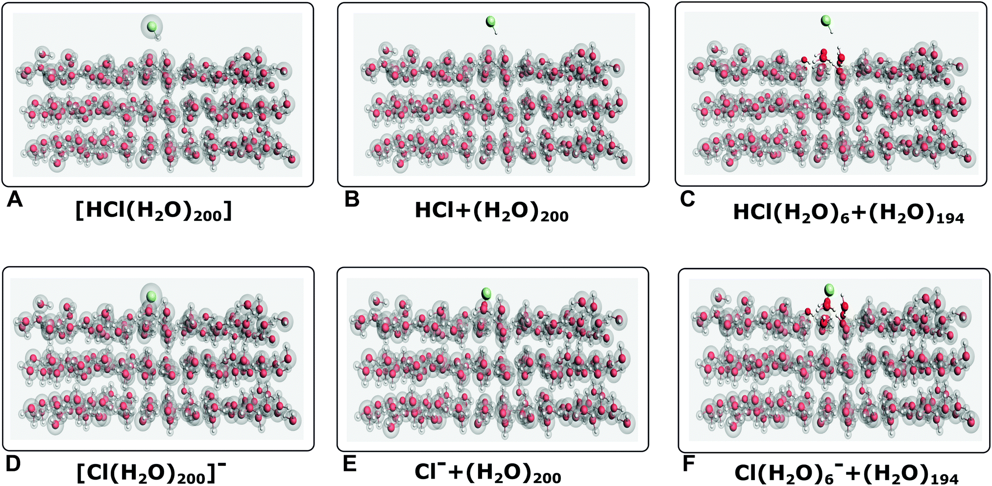

Fig. 1 Perspective views for the cluster models of halogen adsorbed ice surfaces (represented by 200 water molecules): without a partition into the subsystem ((SM, left)), with an active subsystem containing only the halogen (EM1, center) and with an active subsystem containing the halogen and 6 nearest water molecules (EM2 right). Boxes A, B and C represent the system HCl–ice, whereas boxes D, E and F represent the system Cl⁻–ice.

4 Results and discussion

Before proceeding to the discussion of our results for embedding systems, we consider it instructive to address first the performance of theoretical approaches for obtaining core binding energies for the isolated (gas-phase) species, since these provide us with a well-defined reference point with which to assess the behavior of embedded models in complement with a comparison to experimental results.^4,26

4.1 Gas-phase calculations

Our results for gas-phase calculations are shown in Table 1. Considering first the EOM calculations, our choice of focusing on the ²DCG^M Hamiltonian stems from the fact that the Gaunt interaction is essential for appropriately describing the K edge, while showing non-negligible effects for the L edges (see the supplementary result for a comparison to two- and four-component results based on the Dirac–Coulomb Hamiltonian). Here, we also provide an investigation of the basis set convergence with extended basis sets (including an extrapolation to the complete basis set limit) and an in-depth comparison to experimental results. For the SAOP model potential, on the other hand, we are not aware of any comparison for core ionization energies employing the equivalent of the Koopmans theorem for DFT,⁹⁶ that is, by obtaining the core binding energy as the negative of the Kohn–Sham orbital energies (BE = −ε_KS). A Koopmans' approach will be inherently less accurate for core electron binding energies due to the lack of relaxation effects,⁹⁷ though it remains very convenient for a qualitative understanding of chemical shifts for a particular edge. In the case of the SAOP model potential, which has shown a very good performance for valence ionizations of halides and water in droplets,⁶² it is interesting to verify by how much it deviates from EOM calculations for deeper ionizations.

Table 1 CVS-EOM-IP-CCSD chlorine core binding energies (in eV) of HCl and Cl⁻ in the gas phase for the ²DCG^M Hamiltonian employing triple-zeta basis sets and values extrapolated to the complete basis set limit (CBS). In addition to these, we present core binding energies obtained via the analogue of the Koopmans theorem for DFT,⁹⁶ employing the SAOP model for the ZORA Hamiltonian. In parentheses, we present the differences with respect to the CVS-EOM-IP-CCSD ²DCG^M results with triple-zeta basis sets, which we take as the reference. Apart from the energies for the individual edges, we provide the core binding energy shift (Δ_BE, in eV) between HCl and Cl⁻ for the theoretical gas phase values

Species	Hamiltonian	Method	K	L1	L2	L3
HCl	SO-ZORA	SAOP	2764.58 (−69.32)	253.94 (−26.75)	194.08 (−15.94)	192.41 (−15.98)
	^2DCG^M	EOM	2833.90 (0.00)	280.69 (0.00)	210.02 (0.00)	208.39 (0.00)
	^2DCG^M, CBS	EOM	2833.86 (−0.04)	280.79 (0.10)	210.18 (0.16)	208.55 (0.16)
	Exp. (gas phase)^99				208.70	207.1
	Exp. (gas phase)^100				209.01	207.38
Cl^−	SO-ZORA	SAOP	2754.42 (−71.63)	243.88 (−26.93)	184.02 (−16.24)	182.35 (−16.21)
	^2DCG^M	EOM	2824.17 (0.00)	270.73 (0.00)	200.10 (0.00)	198.47 (0.00)
	^2DCG^M, CBS	EOM	2824.13 (−0.04)	270.84 (0.11)	200.29 (0.20)	198.66 (0.19)
	Exp. (NaCl)^102			269.6	200.6	198.9
	Exp. (KCl)^103				200.1	198.6
	Exp. (NaCl)^101		2822.4	270	202	200
Δ BE	SO-ZORA	SAOP	10.16	10.06	10.06	10.06
	^2DCG^M	EOM	9.73	9.96	9.92	9.92
	^2DCG^M	EOM	9.73	9.95	9.89	9.89

---

The present SAOP binding energies correspond to those obtained with the scaled (spin–orbit) ZORA Hamiltonian (we recall that while scaled and unscaled ZORA energies differ significantly for deep cores, the eigenfunctions for both cases are the same⁹⁸). A comparison of the SO-ZORA SAOP and ²DCG^M EOM results shows, unexpectedly, a marked difference between the K, L₁, and L₂/L₃ edges. For the L₂/L₃ edges of both HCl and Cl⁻, the difference between methods is roughly 16 eV, increases to roughly 27 eV for the L₁, and reaches around 70 eV for the K edge, which represent differences in the binding energies of roughly 8–9%, 10% and 2–3% for the respective edges. This difference between SO-ZORA results and EOM is essentially the same for the two species and will be useful for the comparison between structural models that follows.

From the table, we observe that our triple-zeta basis ²DCG^M EOM results overestimate the experimental L₂ and L₃ gas-phase HCl binding energies reported by Hayes and Brown⁹⁹ and Aitken et al.¹⁰⁰ by around 1 eV. A similar difference is observed for the L₁ edge of chloride in the NaCl crystal, with the L₂ and L₃ edges in this case showing deviations smaller than 1 eV. For the K edge, there appears to be a slightly larger discrepancy (around 1.7 eV) between the theory and the experimental values quoted by Thompson et al.¹⁰¹ In spite of the fact that for all edges these experimental results are not for a gas-phase chloride atom, we take the overall very good agreement to indicate that ²DCG^M EOM should show a uniform accuracy for both species.

We note that there remain three potential sources of errors in our calculations: (a) basis set incompleteness; (b) QED and retardation effects; and (c) energy corrections due to higher-order excitations in the CC wavefunctions. For HCl, there could be a fourth, the H–Cl bond distance, but as can be seen from the results of a scan of this coordinate (see the ESI†), even a large variation of bond lengths do not change energies by more than a 0.1–0.2 eV for the L edges and around 0.3 eV for the K edge, meaning that the first three factors should be behind most of the discrepancy.

From the literature,¹⁰⁴ QED and retardation effects are expected to be well below 0.1 eV for chlorine. At this point, we are unable to determine the effect of higher-order excitations with the current implementation in DIRAC. For assessing the basis set effects, we have calculated binding energies with quadruple zeta basis sets and with them and the triple-zeta results obtained the complete basis set limit (CBS) values as shown in Table 1.

Comparing the EOM CBS results to the experimental results of Hayes and Brown⁹⁹ and Aitken et al.¹⁰⁰ for the L₂ and L₃ edges of HCl, we see that agreement gets slightly worse than with the triple-zeta basis, and an interesting point is that for the K edge the effect of extrapolation is to reduce the binding energies whereas for the L edges the opposite is true. For Cl⁻, we see essentially the same variation between the triple zeta and the extrapolated values as for HCl. In both cases, as the L₂ and L₃ edges are affected by the same amounts, the spin–orbit splitting of 2p_1/2 and 2p_3/2 remains at around 1.6 eV for both species, a value consistent with the gas-phase experimental values for HCl (in the NaCl crystal, this splitting is 1.7 eV¹⁰² whereas in KCl it is 1.6 eV¹⁰³).

Finally, we see that the Δ_BE value is nearly indistinguishable, in spite of the calculations having employed different Hamiltonians or correlated methods. This indicates that this is a robust quantity to (semi-quantitatively) characterize the chemical shift in the binding energies, even when the absolute binding energies are rather poor (as is the case of DFT orbital energies).

4.2 Assessing the embedded models

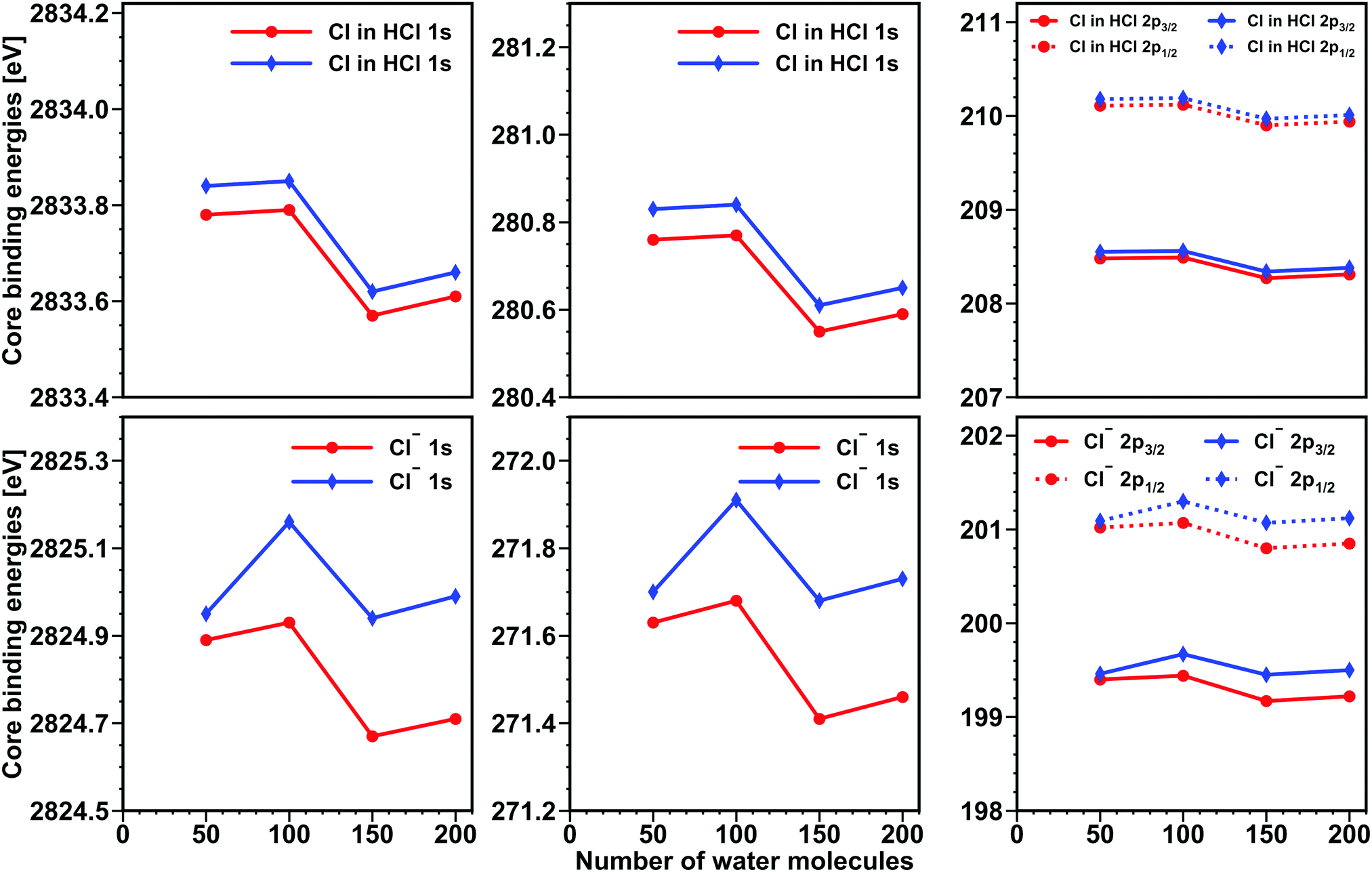
Before proceeding to the calculation of halide binding energies considering the sampling of configurations from MD, it is necessary to make an initial assessment of the quality of the embedding methods and the suitability of the structural models to which we apply the embedding methods. In the first case, the most straightforward evaluation comes from comparing how our embedding models (EM1 and EM2) can reproduce the reference supermolecular model (SM); in the second case, we shall be interested in characterizing the long-range interaction between the halogenated species and its environment.

As discussed in Section 4.1, the ZORA/SAOP model is sufficiently systematic to allow us to compare the behavior of both embedded HCl and Cl⁻ using orbital energies as proxies for the extent to which our embedding models (EM1 and EM2) can reproduce the reference supermolecular model (SM) for the different core edges. From prior studies,^55,62,105 we expect the need for subsystem DFT calculations (in which both the subsystem densities are optimized via freeze–thaw cycles) for Cl⁻, whereas for the neutral HCl FDE calculations (in which the electron density for the environment-the ice surface-is constructed in the absence of the halogen species) relaxation of the environment would be less of an issue,^55,106 and therefore little should be gained from subsystem DFT calculations.

In Fig. 2, we present the comparison, for a selected snapshot, of the different models and how the core binding energies vary as the number of water molecules is included in the Freeze–thaw procedure (for EM1 and EM2 we relax at most the 50 and 40 water molecules nearest to the halogen, respectively). The first important difference between the HCl and Cl⁻ systems is that, as expected, for Cl⁻, there is a much more important change between FDE calculations (zero relaxed water molecules) and subsystem DFT (at least one relaxed water molecule) ones, with FDE calculations with the EM1 model showing discrepancies of around 1.3 eV from the SM for all edges.

Fig. 2 Variations of the approximate K, L₁ and L_2,3 core binding energies of chlorine in HCl (left) and Cl⁻ (right), obtained from scalar ZORA calculations by the SAOP model, with respect to the number of water molecules whose density is relaxed (in the ground state) via freeze–thaw cycles, for models EM1 (squares) and EM2 (circles). For comparison, the corresponding orbital energies obtained for model SM are provided as a reference (dashed line). The L_2,3 values are not split as calculations do not include spin–orbit coupling.

By adding the six nearest water molecule to the active subsystem in EM2, we observe that the difference to SM for FDE is reduced to around 0.8 eV. When 10 water molecules are relaxed, the subsystem DFT calculations with EM1 yield roughly the same results as the FDE ones for EM2, and from this point onwards, both EM1 and EM2 subsystem DFT calculations yield binding energies that differ by around 0.1 eV at most. It is important to note that even after 50 (40) water molecules relaxed, EM1 and EM2 still underestimate the SM binding energies by about 0.5 eV for the L edge and 0.6 eV for the K edge.

For HCl, on the other hand, we see very little improvement over FDE for the subsystem DFT calculations: varying the number of relaxed water molecules from zero to 40 or 50 introduces variations of at most 0.1–0.2 eV. This is in line with our expectation that FDE already provides a rather good representation of the environment for neutral subsystems. In contrast to Cl⁻, we observe that EM2 shows slightly worse agreement to SM than EM1 and that for the L edges the embedding approaches are about 0.1–0.2 eV closer to the reference SM binding energies than for the K edge. In spite of this, embedded models still show rather good agreement to SM, with EM2 typically underestimating the SM binding energies by 0.3 eV for the L edges (and 0.5 eV for the K edge), whereas EM1 reproduces SM binding energies nearly exactly for the L edge while underestimating the K edge binding energies by around 0.2 eV.

Taken together, these results make us confident that, first and foremost, embedded models (and consequently, the underlying embedding potential) are indeed capable of reproducing SM calculations and to do so in a manner that is roughly uniform for the K and L edges alike.

Second, these subsystem DFT derived embedding potentials introduce errors (due to the limited accuracy of the approximate kinetic energy density functionals employed to calculate the non-additive kinetic energy contributions⁴⁸) that should result in small but non-negligible (0.5 eV or lower) underestimation of SM DFT binding energies.

In view of using them in CC-in-DFT calculations, the EM2 model has a significant disadvantage in that the active subsystem is significantly larger than EM1, and given the small difference in performance between the two, here we have opted to focus from now on the EM1 model, and employing the EM2^v model (that contains only one water molecule in the active subsystem instead of six) whenever assessing the suitability of the EM1 model in CC-in-DFT calculations.

In Fig. 3, we employ the EM1 and EM2^v models, again for a single snapshot (and therefore disregard temperature effects introduced by considering several snapshots, as it will be done in the following), to verify the effect of long-range interactions between the halogens and the ice, through the truncation of the size of the water environment in the CC-in-DFT calculations.

Fig. 3 CC-in-DFT K, L₁, L₂ and L₃ triple-zeta binding energies of HCl and Cl⁻ adsorbed on ice surfaces for a single snapshot, as a function of the number of water molecules in the environment (in addition to the 50 molecules nearest to the halogen system that are always taken into account). Blue lines represent the system with only the halogen species in the active subsystem, and red lines represent active systems containing the halogen species and one explicit water molecule.

We observe that for HCl there is no discernible difference between the embedded models, and that long-range effects seem to represent relatively small (0.2 eV) contributions, which are roughly uniform for the different edges, and tend to lower the core binding energies. Interestingly, the plots seem to indicate that long-range effects start to kick in after more than 100 water molecules have been taken into account. For Cl⁻, the situation is qualitatively slightly different, since we see a non-negligible difference between the EM1 and EM2^v CC-in-DFT results, with the latter showing binding energies typically 0.2 eV lower than the former. That is, there appears to be a small decrease in binding energies between 100 and 150 water molecules (0.2 eV), as seen for HCl. We also note that irrespective of the models (EM1 and EM2^v), the splitting between L₂ and L₃ edges remains around 1.6 eV.

Further evidence of the relative insensitivity of the results to the size of the cluster beyond 50 water molecules is given by the analysis of the system's dipole moment as a function of the number of water molecules; as shown in Table S4 in the ESI,† there are no significant changes in dipole for sufficiently large systems.

From these results, we consider that employing the EM1 model is still advantageous from a computational point of view, since we consider that its smaller computational cost offsets the relatively modest improvement brought about by explicitly considering a water molecule in the active subsystem. Furthermore, due to the small changes upon considering a much larger environment, for the following we should only consider models containing the halogen system and 50 water molecules.

4.3 Configurational averaging: ice and droplet models

Having established above that the EM1-based model containing 50 water molecules provides a very good balance between the ability to faithfully reproduce the reference calculations and the computational cost associated with CC-in-DFT calculations, we now turn to a discussion of the effects of the structural model for the environment and of the temperature, both associated with considering snapshots from classical molecular dynamics simulations. Table 2 summarizes our results.

Table 2 Mean values of CC-in-DFT chlorine core binding energies (BEs, in eV) averaged over structures from CMD simulations for models with 50 water molecules, and the difference of BEs and those calculated for the gas phase (Δ^g BE, in eV). The molecular structures correspond to the (A) original CMD snapshots for water droplets⁶² and ice surfaces;⁸⁷ (B) optimization of the halogen system coordinates, keeping the ice surface constrained to the CMD structure; (C) optimization of the halogen system coordinates and four nearest neighbor waters, keeping the remaining of the ice surface constrained to the CMD structure. For the ice surface systems, calculations correspond to a temperature of 210 K. For water droplets, calculations correspond to a temperature of 300 K. We also provide the theoretical results (scalar ZORA SAOP) for valence bands (3a₁ and 1b₁) of water for the ice surface, and for completeness we also provide the CC-in-DFT chlorine 3p for the water droplets and the SAOP water 3a₁ and 1b₁ BEs from the study of Bouchafra et al.,⁶² obtained for the same snapshots as the chlorine BEs. We compare these results to the experimental results by Kong et al.²⁶ (253 K), Parent et al.⁴ (90 K), Partanen et al.¹⁰⁸ (393–423 K), Pelimanni et al.107 (373 K), Kurahashi et al.¹⁰⁹ (280 K) and Winter et al.¹¹⁰

System	Environment	Ionisation	Triple-zeta results
			BE(A)	Δ ^g BE(A)	BE(B)	Δ ^g BE(B)	BE(C)	Δ ^gBE(C)	BE(CBS^a)	Experiment
HCl	Ice	K	2834.03	0.13	2833.40	−0.50	2833.29	−0.61	2834.33	2817.6^26
		L1	280.84	0.15	280.15	−0.54	280.04	−0.65	281.19
		L2	210.18	0.15	209.49	−0.53	209.38	−0.64	210.60	204.9^26
										202.2^4
		L3	208.54	0.15	207.86	−0.53	207.75	−0.64	209.04	202.8^26
										200.9^4
Cl^−		K			2827.70	3.53			2828.79	2815.4^26
		L1			274.90	4.17			275.07
		L2			204.41	4.31			204.47	202.7^26
										199.6^4
		L3			202.70	4.23			202.91	200.6^26
										198.3^4
		3p								10^4
Cl^−	Droplet	K	2829.97	6.66					2829.93
		L1	276.63	5.90					276.74
		L2	205.99	5.89					206.19	205.0^107
										205.0^108
										202.7^26
		L3	204.36	5.89					204.55	203.4^107
										203.4^108
										200.6^26
		3p1/2	9.9^62						10.1^62
		3p3/2	9.7^62						9.9^62	9.8^107
										9.5^109
										9.6^110
H2O	Cl^− ice	3a1	16.1							13.7^4
		1b1	12.6							12^4
	Droplet	3a1	12.5^62							13.76^108
										13.78^109
										13.50^110
		1b1	10.4^62							11.4^107
										11.41^108
										11.31^109
										11.16^110

---

Starting with the chloride ion in a droplet we observe that our calculated triple-zeta quality binding energies (BE(A), calculated from the average of binding energies over 100 snapshots of a simulation at 300 K) show a slightly larger shift with respect to the gas-phase value (Δ^g BE(A)) for the K edge (around 6.7 eV) than that for the L edges (around 5.9 eV), which is consistent with the picture from our analysis of the single snapshot ZORA/SAOP results in Section 4.2. We have not carried out quadruple zeta calculations for this system, due to the fact that the CBS corrections to the triple-zeta values for the chloride–ice surface (see ESI†), at least for the L edges, are rather similar to the ones obtained for the gas-phase system. As such, we have decided to apply the gas-phase corrections for both the K and L edges to the droplet system, given that for valence ionizations⁶² CBS corrections from the gas-phase or from averaged droplet binding energies were essentially the same.

A comparison of the droplet CBS-corrected values to the experimental results of Pelimanni et al.,¹⁰⁷ which have measured the L₂ and L₃ edges for KCl solutions at different concentrations and somewhat higher temperatures (nozzle temperature of 373 K), shows that our results are in good agreement with the experiment, as our results overestimate the experiment by almost exactly 1 eV for each edge.

Our 2p spin–orbit splitting is consistent with that of the experiment, at around 1.6 eV, a value that is close to the one seen in the gas phase (roughly the same differences are found in comparison to the experimental results of Partanen et al.¹⁰⁸). There are much more significant discrepancies between our simulations and the experimental results of Kong et al.²⁶ obtained at somewhat lower temperatures (253 K), not only in terms of the binding energy values (which are around 4 eV lower than our results) but also of the 2p spin–orbit splitting (2.1 eV), which is 0.5 eV larger than both our simulation and other experimental results.^107,108

The discrepancy between our results and those of Kong et al. could be due to temperature effects, since encapsulation of the halogens is driven by the temperature induced surface disorder, though the role of other parameters such as differences in calibrations in the BE scale, cannot be dismissed out of hand. We note that Kong et al. have used the oxygen K edge as the internal reference, but since obtaining such data is beyond the scope of this work (as it would require the construction and validation of new embedding models in order to carry out CC-in-DFT calculations on water molecules), we provide the results for the valence band of water for the droplet model in Table 2, obtained from SAOP orbital energies by Bouchafra et al.⁶²

As discussed in the original work, the SAOP valence band of water obtained from calculations on droplet models is quite consistent with the available experimental results, with the 1 eV underestimation of experimental values having to do with the size of the water droplet (50 water molecules) employed by Bouchafra et al. The good agreement between our theoretical values and the experimental values of Pelimanni et al. not only for the valence band of water, but also for the valence band of chloride, make us confident in the reliability of our embedded models and the CC-in-DFT protocol for core edges.

Considering now the chloride ion at the ice surface, our calculated triple-zeta quality binding energies (BE(B), calculated from the average of binding energies over 25 snapshots obtained by a combination of MD simulations at 210 K for HCl, followed by the optimisation of the chlorine atom position) show similar behavior to that of droplets with respect to the free ion, with Δ^g BE(B) values which are nearly the same for the K and L edges, again in line with the picture that the embedding potentials for these calculations affect the K and L edges in a roughly homogeneous manner. Here, however, we have a smaller shift for the K edge (3.53 eV) than that for the L edges, and for the latter the differences between L₁, L₂ and L₃ are of the order of 0.1 eV, that is, an order of magnitude more than that for the water droplet.

In qualitative terms, our calculations reproduce well the trend of decreasing binding energies when going from the solution represented by the experimental results of Pelimanni et al.¹⁰⁷ to the surface represented by the experimental results of Parent et al.⁴ for lower temperatures and Kong et al.²⁶ for higher temperatures (though, for the latter, a near equivalence between the reported chloride binding energies of NaCl solution and ice surface at 253 K would indicate that chloride does behave as a free ion in both systems).

Quantitatively, our CBS corrected triple zeta results show differences in the order of 4 eV for the L₂ and L₃ edges with respect to the experimental results of Parent et al.,⁴⁴ obtained at 90 K. At the same time, the water valence band for the theoretical model for the ice surface is in good agreement with the same low-temperature experiment, with discrepancies of around 0.6 eV for the 1b₁ band. For the 3a₁ band, discrepancies are of about 2 eV, but experimentally that is a broader band and therefore more difficult to provide an unambiguous comparison between the theory and experiment. The difference of the performance of our models for the ice surface valence binding energies and the core chloride binding energies could be an indication of the importance of temperature effects, which cannot be properly accounted for in our models since we only have data at 210 K.

The discrepancies for core BEs are smaller with respect to the results of Kong et al.,²⁶ measured at 253 K (and thus closer to the simulation conditions), but our values still overestimate the experimental results by 1.77 eV and 2.31 eV for the L₂ and L₃ edges, respectively. This is larger than the differences we observe for droplets between the theory and the results of Pelimanni et al.,¹⁰⁷ but somewhat smaller than the differences between our droplet model and the results for NaCl solution from the study of Kong et al.²⁶ In our view, taken together the results for Cl⁻ on ice and water droplets seem to indicate a fairly systematic difference between our theoretical models and the experimental results of Kong et al.

On the simulation side, there is an important difference between the chloride–ice system with respect to the droplets, which is linked to the process and quality of the sampled structures, since the sampling is intimately connected to the description of temperature effects. By observing Fig. 4, in which we show the K and L edge binding energies obtained for each snapshot around the mean value presented in Table 2, we see narrow distributions around the mean for the droplet system for all edges considered (within envelopes of around 1 to 1.5 eV). For the chloride–ice system, the distributions are much wider, and around 3 eV for the L edges and almost 10 eV for the K edge.

Fig. 4 CC-in-DFT K, L₁, L₂ and L₃ triple-zeta binding energies of chloride adsorbed on ice surfaces at 210 K (results averaged over 25 snapshots) and in water droplets at 300 K (results averaged over 100 snapshots).

This difference is in part expected, since, in the droplet model, the chloride ion is always completely surrounded by water molecules, and therefore one can consider that on average the ion has always a fairly constant degree of interaction with its environment, whereas, for the ice model, the amount of water molecules with which the ion interacts greatly depends on how much it has penetrated into the QLL. We speculate that, in our case, the sampled structures place the chloride ion deeper than it would be on average and with that our results could be overestimating the chloride–surface interaction and, consequently, yielding an artificial increase in core binding energies, due to the fact that waters do not relax when the ion is introduced.

It may also be that our configurations are not properly representing the local environment of the chloride ion, as probed by the spin–orbit splitting of the 2p, though here the current experimental and theoretical data, in our view, do not allow for any definitive conclusions. In one hand, Kong et al.²⁶ obtained an experimental difference between the L₂ and L₃ edges of 2.1 eV. On the other hand, our calculated splitting for chloride–ice is of roughly 1.7 eV, a value consistent with splitting between the L₂ and L₃ edges in the NaCl crystal (see Table 1) and slightly larger than that of roughly 1.6 eV we obtained for the gas-phase ion, our droplet results and the experimental work of Pelimanni et al.¹⁰⁷ founnd for the solvated ion. It is also interesting to note that the 2.1 eV splitting is much larger than the 1.3 eV splitting observed by Parent et al.,⁴⁴ that is closer to our results.

In the case of the K edge, a problem with adequate sampling could be the reason for our large overestimation of the experimental binding energies, since from Fig. 4 we see that K edge energies are extremely sensitive to the configuration. At this stage, we lack a better classical polarizable force field that can represent both the water–chloride and water–water interactions in the ice QLL. Due to this, the question of whether (and if so, how) better sampling would affect the K edge remains an open question.

Unlike the two chloride systems discussed above, for HCl a straightforward use of the molecular dynamics simulation snapshot yields results which are essentially the same as those for the isolated molecule. This indicates that in these snapshots there are, in effect, all but residual interactions between HCl and the ice (Δ^g BE(A) values are very small and around 0.15 eV for all edges). By observing the top of Fig. 5, this becomes quite clear: in spite of averaging over 25 snapshots, there is essentially no spread in binding energy values, which would otherwise be the case if there were stronger interactions with the surface. This is consistent with the findings of Woittequand et al.¹¹¹ that the adsorption energy of HCl on ice (of the order −0.2 eV) is quite small in the absolute value.

Fig. 5 CC-in-DFT chlorine K, L₁, L₂ and L₃ triple-zeta binding energies for HCl adsorbed on ice surfaces at 210 K (results averaged over 25 snapshots) employed as structural models: (A) the original CMD snapshots (top); (B) reoptimizing the HCl molecule while constraining the ice surface to retain the atomic positions of model A (middle); and (C) reoptimizing the HCl and four nearest water molecules, while constraining the rest of the ice surface to retain the atomic positions of model A (bottom).

If we take the snapshots as starting points for geometry optimizations of the HCl molecule, keeping the ice structure constrained to the original CMD configurations, we see a small but non-negligible change in the binding energies (BE(B)) for the different edges, so that now instead of the slight increase of binding energies seen at first, we start to see a move towards lower binding energies ((Δ^g BE(B) of about −0.50 eV)), that is, towards the experimental trend (HCl on ice binding energies being lower than gas-phase ones). Similar to chloride on the ice system, there is a large spread in values (of around 2–3 eV for the K and L edges, see the middle of Fig. 5).

Upon obtaining configurations in which we also optimize the waters nearest to the HCl molecule, we observe a further decrease in binding energies (BE(C)) that, though in the direction of experiment, is too small to bring our calculations to the same agreement with experiment as seen for the L edges of the chloride–ice system discussed above, and we see discrepancies of around 5.7–6 eV. The discrepancy between the theory and experiment for HCl–ice K edge binding energies is also around 3 eV larger than that for the chloride–ice system.

One possible issue with these simulations on ice is that, at 210 K, the temperature of the simulations is somewhat lower than that of the experiment. This makes it worthwhile to explore the effect of the temperature on the ice structures, and see to which extend the changes would affect the binding energies.

To this end, we have carried out additional classical MD simulations for HCl under the same conditions as performed for 210 K, one at 235 K and another at 250 K, and selected a single snapshot of each to carry out exploratory CC-in-DFT calculations. In Fig. S1 and S2 (ESI†), we show respectively the structures of HCl and Cl⁻ at the two temperatures.

From these figures, and keeping in mind the structures at 210 K shown in Fig. 1, we see the progressive disorganization of the upper layers of the interface when moving from 210 K to 235 K (though the innermost two layers remain rather well structured), and a fairly substantial loss of structure moving from 235 K to 250 K.

In spite of these significant changes in the structure, between the different temperatures, there are little changes to the binding energies, as can be seen from Table S5 in the ESI.† Even though we have only one structure, and therefore we cannot strictly compare to the averaged results for 210 K, the results in Table S5 (ESI†) suggest nevertheless that temperature effects cannot play a major role in modifying the binding energies if the HCl molecule remains essentially bound (and with an internuclear distance not far from the gas-phase value), as we discuss in the following.

4.4 A closer look on the HCl–water interaction

The contrast between the chloride and HCl results and the changes (albeit modest) in binding energies observed for HCl depending on the strucural model for the HCl–ice surface interaction sites discussed above, a call for a closer look at how the structural parameters affect the calculated binding energies, as shown in Fig. 6. Considering first the HCl internuclear distance (panel D), we see that for the original snapshots from the CMD simulations of Woittequand et al.⁸⁷ (model A), one obtains essentially the same binding energies which, as discussed above, are nearly indistinguishable from the gas-phase ones.

Fig. 6 Scalar ZORA chlorine 2p binding energies as a function of the HCl–H₂O intra- and inter-molecular distances of HCl adsorbed on ice surfaces at 210 K for the 25 snapshots, employed as structural models: (A) the original CMD snapshots; (B) reoptimizing the HCl molecule while constraining the ice surface to retain the atomic positions of model A; and (C) reoptimizing the HCl and four nearest water molecules, while constraining the rest of the ice surface to retain the atomic positions of model A. In panel D, the BEs with respect to the HCl bond lengths in models A, B and C are shown.

Upon optimizing the HCl position while keeping the surface unchanged (model B), we see a significant change in that internuclear distances increase for all snapshots with respect to model A, to values between 1.28 and 1.38 Å; furthermore, we can identify three categories of points: those for internuclear distances around 1.28 Å, which are associated with larger core binding energies (right of the figure), those for internuclear distances between 1.32 and 1.36 Å, which are associated with lower core binding energies (left of the figure), and the third cluster for internuclear distances between 1.28 and 1.34 Å, but which exhibit roughly the core same binding energies (around 208 eV).

The optimization of the HCl and nearest water molecules (model C) accentuates somewhat the trend of increased internuclear distances in the region for lower core binding energies seen for model B. We observe more snapshots with internuclear distances larger than 1.36 Å, which are 1 to 2 eV lower than the core binding energies for model A (and we note that, in contrast to the gas-phase results, relatively small changes in the internuclear distance produce a significant shift of core binding energies). However, the average core binding energy only shows modest changes with respect to model A due to the fact that there remain several structures with core binding energies larger than 208.5 eV.

Apart from the H–Cl distance, we see significant changes in the distances between the hydrogen in HCl and the nearest oxygen atoms of the surface: while, for model A, the large variation in this O–H distance does not significantly affect the binding energies, for models B and C we can distinguish two types of distances: longer ones (around 3.5 Å) for which the core binding energies are generally above 208 eV, and shorter ones (around 1.6 Å) associated with lower core binding energies.

Taken together, these observations suggest that the lowering of the core binding energies is closely connected to the concerted increase in the HCl internuclear distance and decrease of the oxygen surface atoms and the hydrogen of HCl, which would represent the initial stage of the (pre)dissociation of HCl mediated by the surface. Two such configurations can be more clearly visualized in Fig. 7, which depicts the spatial arrangement of HCl and its nearest four water molecules for two situations in which structural relaxation is taken into account. The figure also contains the core binding energies obtained for each microsolvated cluster. We observe that, already in such simplified models, binding energies are quite sensitive for relatively small changes in the structure. One can also identify in the figure cooperative effects coming from the elongation of certain O–H bonds in the water molecules as the HCl molecule gets closer (with the elongation of the H–Cl bond and the interaction of the hydrogen of HCl and the oxygen of the nearest water). A further investigation of the influence of predissociation of HCl would require more extensive CMD simulations for the surface, which are beyond the scope of this work.

Fig. 7 Structures for a microsolvated HCl molecule originating from a snapshots of model C, with nearest 4 waters shown. Internuclear distances (in Å) are indicated in the figure. Binding energies (in eV) for the [K, L₁, L₂, and L₃] edges, obtained with CC-in-DFT (for the microsolvated system) are respectively [2832.6, 279.3, 208.7, and 207.1] (top) and [2831.9, 278.7, 208.0, and 206.4] (bottom).

To further explore this point, we have considered two additional models: (a) one in which a +1 point charge is placed at a given distance r from the chloride ion; and (b) one in which we employ one snapshot of the chloride droplet model to construct a HCl droplet model, by placing the added hydrogen atom near the chloride or a given oxygen (to simulate the H₃O⁺ species), and performing a constrained optimization (fixing all atoms but the hydrogens belonging to the same species the hydrogen has been attached to). The results for these models are found in Table 3 and Table S6 of the ESI.†

Table 3 Core binding energy shifts (Δ_BE, in eV) between the Cl⁻ and HCl systems as a function of the distance r (in Å) between the chlorine and hydrogen atoms, for (a) the electrostatic gas-phase model based on the pair of charges (chloride and a +1 point charge representing the hydrogen); and (b) the [HCl(H₂ O)₅₀] droplet model structure based on the [Cl(H₂O)₅₀]⁻ droplet model discussed above, in which the additional hydrogen is found near the different heavy centers (chlorine and oxygen). See the text and the ESI for further details and approximate core electron binding energies

r	Core binding energies
	Droplet model			Gas-phase model
	K	L1	L2/L3	K	L1	L2/L3
1.306	7.48	7.53	7.69	8.59	8.73	8.80
2.559	3.05	3.06	3.05	5.70	5.71	5.75
3.489	2.81	2.81	2.82	4.16	4.17	4.18
5.690	2.32	2.33	2.33	2.53	2.53	2.54
10.256	1.60	1.64	1.64	1.40	1.40	1.40

---

Starting with the gas-phase model (a), we observe that at distances slightly larger than the gas-phase equilibrium (r = 1.306 Å), the Δ_BE values are rather close to the values for the molecular HCl system (8.6–8.8 eV vs. roughly 10 eV in Table 1). As r is increased to r = 2.559 Å, the distance already much larger than those sampled by our MD simulations and shown in Fig. 6 and 7, there is a significant decrease in Δ_BE to 5.7 eV, and then a relatively smooth decrease for larger distances. Interestingly, at around r = 5.690 Å, Δ_BE decreases to around 2.5 eV, which is in the order of magnitude of the experimental chemical shift reported by Kong et al.²⁶ (2.2 eV) and also close to the value by Parent et al.⁴ (2.6 eV). While not shown, we have investigated how far the +1 point charge would have to be in order for us to obtain the gas-phase Cl⁻ value, and at r = 100 Å there are still small differences (around 0.1 eV).

For model (b), we have the same qualitative trend, but with an interesting difference: while the Δ_BE value at r = 1.306 Å is still relatively large (around 7.5 eV), comparing it with the gas-phase Δ_BE value shown in 2, we can infer an environment effect of around 2.5 eV, which is already much larger than the effects shown in Table 2 and in line with Fig. 6 and 7. For r = 2.559 Å, due to the effect of the screening by the water molecules in the droplet (see Fig. S3 in the ESI†), the Δ_BE value (around 3 eV) is nearly 3 eV lower than the one from the gas-phase. Likewise, at r = 3.489 Å, the Δ_BE value is already below 3 eV (and a little over 1 eV smaller than the gas-phase value).

For larger r values, model (b) follows roughly the behavior of model (a), which may be due to the small size of the droplet. In contrast to the gas-phase model, our simulations do not allow us to probe much longer distances than 10 Å, but the relative small difference to the anionic systems suggests in our view that the anionic systems would be indeed rather good models for diluted solutions. In a subsequent work, it will be interesting to investigate how screening will alter the rate of convergence towards the anionic result, now that polarizable force fields of similar accuracy to those employed here and that can handle counter ions are starting to become available.¹¹²

Whatever the case, these results suggest that, for a solvated system, chemical shifts compatible to those observed in the experiment occur for values of r between 4 and 6 Å.

While these results only consider single structures, and therefore must be viewed as providing semi-quantitative evidence, they help in understanding the poor agreement with the experiment for the simulations of HCl on ice shown in Table 2 likely comes from an inadequate structural model, which assumes and retains a bound (molecular) picture for HCl, when it would seem that a more suitable situation resembles the existence of an ion pair, or some other intermediate situation. Unfortunately, we do not currently possess the adequate tools to further explore this problem, and in any case such an undertaking requires a dedicated study.

5 Conclusions

In this article, we report the application of the relativistic CVS-EOM-IP-CCSD-in-DFT approach to obtain the core electron binding energies of chlorinated species (Cl⁻ and HCl) at the air–ice interface which is of great interest for atmospheric chemistry and physics, as well as of Cl⁻ in aqueous solution (which allows us to differentiate isotropic and nonisotropic solvation of the anion). In our coupled cluster calculations, we employ the molecular mean-field Dirac–Coulomb–Gaunt Hamiltonian, which accurately accounts for spin-same orbit and spin-other orbit interactions.

These calculations are based on structural models considering, for both droplets and ice surfaces, the halides and the nearest 50 and 200 water molecules, respectively. Based on these, embedding models in which all water molecules were treated at the DFT level while the halide species were treated with the coupled cluster have been assessed, and their relative accuracy verified against reference DFT calculations on the whole system. Therefore, we have found that subsystem DFT calculations, in which both the halide and 50 nearest water molecules in the environment were relaxed in the presence of each other, were well-suited for both the neutral (HCl) and the charged (Cl⁻) subsystems, showing small and systematic errors for all edges.

The accuracy of our protocol has been shown for the water droplet case, for which we obtain L₂ and L₃ CBS-corrected core binding energies in very good agreement but overestimate the most recent experiments by Pelimanni et al.¹⁰⁷ in solution by around 1 eV for each edge, while obtaining nearly the same energy splitting (1.66 eV, due to spin–orbit coupling) as the experiment (1.6 eV) between the L₂ and L₃ edges. We consider that remaining discrepancies are likely due, in part, to the different temperatures in which the theoretical and experiment results have been obtained and also due to the lack of corrections for higher excitations in our calculations.

Our theoretical values for the L edges of chloride on ice surfaces show systematic differences to the droplet model (binding energies roughly 1.7 eV smaller). They are also in fairly good agreement with the experiment for the L₂ and L₃ edges, though with larger discrepancies than for water droplets, with theoretical values overestimating the experiment by 1.8 and 2.3 eV, respectively.

While this may partially arise from the shortcomings of our protocol to obtain structures for chloride (classical MD simulations on HCl followed by the constrained geometry optimization of the chloride position, due to the lack of suitable force fields), it should be pointed out that our theoretical spin–orbit splitting between the L₂ and L₃ edges is consistent (1.56 eV) with that in the droplet model, with experiments in solution and in the NaCl crystal. The experimental splitting on ice reported by Kong et al.,²⁶ on the other hand, is somewhat larger (2.1 eV) and advantages to be further investigated from both a theoretical and an experimental point of view.

For the K edge, we observe that chloride binding energies on ice are 1.1 eV smaller than those in the droplet model, qualitatively in line with the results for the L edges and with the overall experimental trend of lowering the core binding energies when moving from a solution to a surface for chloride. However, the theory strongly overestimates (by 13.4 eV) the experimental K edge binding energies. At this stage, we cannot pinpoint the factor(s) driving this discrepancy, though we note that, in contrast to the droplet model, there are very significant variations in the K edge binding energies depending on the snapshot used. In our view, this calls for additional simulations once a better force field for the MD simulations is available, in order to confirm whether or not the configuration sampling is a significant source of bias to the theoretical binding energies. However, at this point, we are not equipped to carry out such simulations.

We also report estimates for the valence binding energy of water in the ice surfaces, which are in good agreement with experiments at low temperatures. For this, we have followed the procedure previously employed for obtaining the water valence band for water in droplets, in which the use of the SAOP model potential to describe the environment yields valence binding energies as a by-product of the setup of the embedded coupled cluster calculations at no additional cost.

In contrast to the chloride results, our results for molecular HCl on ice surfaces show poor quantitative agreement with the experiment. We obtain core binding energies that are significantly higher than experimental ones (nearly 6 eV for the L edges, and nearly 17 eV for the K edge), due to the fact that there are almost negligible environmental effects and, therefore, the results are essentially the same as those for gas-phase HCl.

We have assessed to a limited extent the importance of temperature effects on the binding energies by comparing the CC-in-DFT core binding energies based on single structures taken from classical MD simulations of HCl at higher temperatures (235 K and 250 K) to those averaged over 25 snapshots at 210 K. We found that, in spite of the important disorganization of the ice structure as the temperature increases, there are no significant changes in the binding energies of Cl in HCl.

From an analysis of small microsolvated clusters and of two models to capture the variation of the core binding energies as a function of the H–Cl distance (a simple gas-phase one, and droplet models for HCl constructed from the chloride droplet model shown to be reliable), we were able to trace the root cause of this lack of sensitivity to the environment to the inability of our structural models to account for the (pre)dissociation of the HCl molecule upon the interaction with water molecules around it, resulting in the transfer of the proton to the first and second solvation layers.

In spite of their limitations, and notably the lack of any configurational averaging, the gas-phase electrostatic and HCl droplet models provide evidence that, in order to be consistent with the experimentally observed chemical shifts between chloride and HCl of about 2.2–2.6 eV, the proton in the latter should be likely distant from the chlorine atom by around 5–6 Å, a situation which is compatible with it participating in the hydrogen bond network. As such, perhaps a more suitable description for HCl on ice is that of an ion pair rather than of a molecular species. In order to properly characterize this system, it appears to us that a central ingredient would be a MD approach that could (at least) approximately account for such an ion-pair formation, and ideally describe the exchange of hydrogens between different water molecules, but such studies fall outside the scope of this work.

Conflicts of interest

There are no conflicts to declare.

Acknowledgements

We acknowledge support by the French government through the Program “Investissement d'avenir” through the Labex CaPPA (contract ANR-11-LABX-0005-01), the I-SITE ULNE project OVERSEE and MESONM International Associated Laboratory (LAI) (contract ANR-16-IDEX-0004), the Franco-German project CompRIXS (Agence nationale de la recherche ANR-19-CE29-0019, Deutsche Forschungsgemeinschaft JA 2329/6-1), the CPER CLIMIBIO (European Regional Development Fund, Hauts de France council, French Ministry of Higher Education and Research) and the French national supercomputing facilities (grants DARI A0070801859, A0090801859 and A0110801859).

Notes and references

1. S. Solomon, Rev. Geophys., 1999, 37, 275–316.
2. J. P. Abbatt, Chem. Rev., 2003, 103, 4783–4800.
3. T. F. Kahan and D. Donaldson, Environ. Sci. Technol., 2010, 44, 3819–3824.
4. P. Parent, J. Lasne, G. Marcotte and C. Laffon, Phys. Chem. Chem. Phys., 2011, 13, 7142–7148.
5. A. Křepelová, T. Huthwelker, H. Bluhm and M. Ammann, Chem. Phys. Chem., 2010, 11, 3859–3866.
6. J. T. Newberg and H. Bluhm, Phys. Chem. Chem. Phys., 2015, 17, 23554–23558.
7. J. P.-D. Abbatt, J. L. Thomas, K. Abrahamsson, C. Boxe, A. Granfors, A. E. Jones, M. D. King, A. Saiz-Lopez, P. B. Shepson, J. Sodeau, D. W. Toohey, C. Toubin, R. von Glasow, S. N. Wren and X. Yang, Atmos. Chem. Phys., 2012, 12, 6237–6271.
8. J. D. Smith, R. J. Saykally and P. L. Geissler, J. Am. Chem. Soc., 2007, 129, 13847–13856.
9. P. N. Perera, B. Browder and D. Ben-Amotz, J. Phys. Chem. B, 2009, 113, 1805–1809.
10. S. Hüfner, Photoelectron spectroscopy: principles and applications, Springer Science & Business Media, 2013.
11. H. Tissot, G. Olivieri, J.-J. Gallet, F. Bournel, M. G. Silly, F. Sirotti and F. Rochet, J. Phys. Chem. C, 2015, 119, 9253–9259.
12. I. Gladich, S. Chen, M. Vazdar, A. Boucly, H. Yang, M. Ammann and L. Artiglia, J. Phys. Chem. Lett., 2020, 11, 3422–3429.
13. L. Partanen, M.-H. Mikkelä, M. Huttula, M. Tchaplyguine, C. Zhang, T. Andersson and O. Björneholm, J. Chem. Phys., 2013, 138, 044301.
14. S. K. Eriksson, I. Josefsson, N. Ottosson, G. Ohrwall, O. Bjorneholm, H. Siegbahn, A. Hagfeldt, M. Odelius and H. Rensmo, J. Phys. Chem. B, 2014, 118, 3164–3174.
15. K. H. Kim, J. H. Lee, J. Kim, S. Nozawa, T. Sato, A. Tomita, K. Ichiyanagi, H. Ki, J. Kim and S.-I. Adachi, et al. , Phys. Rev. Lett., 2013, 110, 165505.
16. S. Yamamoto, T. Kendelewicz, J. T. Newberg, G. Ketteler, D. E. Starr, E. R. Mysak, K. J. Andersson, H. Ogasawara, H. Bluhm and M. Salmeron, et al. , J. Phys. Chem. C, 2010, 114, 2256–2266.
17. J. T. Newberg, D. E. Starr, S. Yamamoto, S. Kaya, T. Kendelewicz, E. R. Mysak, S. Porsgaard, M. B. Salmeron, G. E. Brown Jr and A. Nilsson, et al. , Surf. Sci., 2011, 605, 89–94.
18. P. D. Dau, J. Su, H.-T. Liu, J.-B. Liu, D.-L. Huang, J. Li and L.-S. Wang, Chem. Sci., 2012, 3, 1137–1146.
19. A. Krepelova, T. Bartels-Rausch, M. A. Brown, H. Bluhm and M. Ammann, J. Phys. Chem. A, 2013, 117, 401–409.
20. G. Olivieri, A. Goel, A. Kleibert, D. Cvetko and M. A. Brown, Phys. Chem. Chem. Phys., 2016, 18, 29506–29515.
21. A. P. Gaiduk, M. Govoni, R. Seidel, J. H. Skone, B. Winter and G. Galli, J. Am. Chem. Soc., 2016, 138, 6912–6915.
22. D. E. Starr, M. Favaro, F. F. Abdi, H. Bluhm, E. J. Crumlin and R. van de Krol, J. Electron Spectrosc. Relat. Phenom., 2017, 221, 106–115.
23. N. K. Jena, I. Josefsson, S. K. Eriksson, A. Hagfeldt, H. Siegbahn, O. Björneholm, H. Rensmo and M. Odelius, Chem. – Eur. J., 2015, 21, 4049–4055.
24. V. F. McNeill, T. Loerting, F. M. Geiger, B. L. Trout and M. J. Molina, Proc. Natl. Acad. Sci. U. S. A., 2006, 103, 9422–9427.
25. V. F. McNeill, F. M. Geiger, T. Loerting, B. L. Trout, L. T. Molina and M. J. Molina, J. Phys. Chem. A, 2007, 111, 6274–6284.
26. X. Kong, A. Waldner, F. Orlando, L. Artiglia, T. Huthwelker, M. Ammann and T. Bartels-Rausch, J. Phys. Chem. Lett., 2017, 8, 4757–4762.
27. K. Bolton, THEOCHEM, 2003, 632, 145–156.
28. S.-C. Park and H. Kang, J. Phys. Chem. B, 2005, 109, 5124–5132.
29. P. Parent and C. Laffon, J. Phys. Chem. B, 2005, 109, 1547–1553.
30. J. Stanton and R. Bartlett, J. Chem. Phys., 1993, 98, 7029–7039.
31. K. Sneskov and O. Christiansen, Wiley Interdiscip. Rev.: Comput. Mol. Sci., 2012, 2, 566–584.
32. R. J. Bartlett, Wiley Interdiscip. Rev.: Comput. Mol. Sci., 2012, 2, 126–138.
33. A. I. Krylov, Ann. Rev. Phys. Chem., 2008, 59, 433–462.
34. O. Christiansen, P. Jørgensen and C. Hättig, Int. J. Quantum Chem., 1998, 98, 1.
35. H. Koch and P. Jørgensen, J. Chem. Phys., 1990, 93, 3333–3344.
36. S. Coriani, F. Pawlowski, J. Olsen and P. Jørgensen, J. Chem. Phys., 2016, 144, 024102.
37. L. S. Cederbaum, W. Domcke and J. Schirmer, Phys. Rev. A: At., Mol., Opt. Phys., 1980, 22, 206–222.
38. S. Coriani and H. Koch, J. Chem. Phys., 2015, 143, 181103.
39. S. Coriani and H. Koch, J. Chem. Phys., 2016, 145, 149901.
40. A. Sadybekov and A. I. Krylov, J. Chem. Phys., 2017, 147, 014107.
41. M. L. Vidal, X. Feng, E. Epifanovsky, A. I. Krylov and S. Coriani, J. Chem. Theory Comput., 2019, 15, 3117–3133.
42. L. Halbert, M. L. Vidal, A. Shee, S. Coriani and A. S.-P. Gomes, J. Chem. Theory Comput., 2021, 17, 3583.
43. T. Saue, Chem. Phys. Chem., 2011, 12, 3077–3094.
44. J. Sikkema, L. Visscher, T. Saue and M. Iliaš, J. Chem. Phys., 2009, 131, 124116.
45. X. Zheng and L. Cheng, J. Chem. Theory Comput., 2019, 15, 4945–4955.
46. J. Lee, D. W. Small and M. Head-Gordon, J. Chem. Phys., 2019, 151, 214103.
47. A. S.-P. Gomes and C. R. Jacob, Annu. Rep. Section C (Physical Chemistry), 2012, 108, 222–277.
48. C. R. Jacob and J. Neugebauer, Wiley Interdiscip. Rev.: Comput. Mol. Sci., 2014, 4, 325–362.
49. T. A. Wesołowski, Phys. Rev. A: At., Mol., Opt. Phys., 2008, 77, 012504.
50. F. Libisch, C. Huang and E. A. Carter, Acc. Chem. Res., 2014, 47, 2768–2775.
51. T. A. Wesolowski, S. Shedge and X. Zhou, Chem. Rev., 2015, 115, 5891–5928.
52. Q. Sun and G. K.-L. Chan, Acc. Chem. Res., 2016, 49, 2705–2712.
53. D. V. Chulhai and J. D. Goodpaster, J. Chem. Theory Comput., 2018, 14, 1928–1942.
54. B. Hegely, P. R. Nagy and M. Kallay, J. Chem. Theory Comput., 2018, 14, 4600–4615.
55. A. S.-P. Gomes, C. R. Jacob and L. Visscher, Phys. Chem. Chem. Phys., 2008, 10, 5353–5362.
56. S. J. Bennie, B. F. Curchod, F. R. Manby and D. R. Glowacki, J. Phys. Chem. Lett., 2017, 8, 5559–5565.
57. S. Prager, A. Zech, T. A. Wesolowski and A. Dreuw, J. Chem. Theory Comput., 2017, 13, 4711–4725.
58. S. Hofener and L. Visscher, J. Chem. Theory Comput., 2016, 12, 549–557.
59. D. J. Coughtrie, R. Giereth, D. Kats, H.-J. Werner and A. Kohn, J. Chem. Theory Comput., 2018, 14, 693–709.
60. S. Höfener, A. S.-P. Gomes and L. Visscher, J. Chem. Phys., 2013, 139, 104106.
61. C. Daday, C. König, J. Neugebauer and C. Filippi, Chem. Phys. Chem., 2014, 15, 3205–3217.
62. Y. Bouchafra, A. Shee, F. Réal, V. Vallet and A. S.-P. Gomes, Phys. Rev. Lett., 2018, 121, 266001.
63. A. Sadybekov and A. I. Krylov, J. Chem. Phys., 2017, 147, 014107.
64. S. Höfener, A. Severo Pereira Gomes and L. Visscher, J. Chem. Phys., 2012, 136, 044104.
65. V. Parravicini and T.-C. Jagau, Mol. Phys., 2021, e1943029.
66. T. A. Wesolowski and A. Warshel, J. Phys. Chem., 1993, 97, 8050–8053.
67. T. Dresselhaus, J. Neugebauer, S. Knecht, S. Keller, Y. Ma and M. Reiher, J. Chem. Phys., 2015, 142, 044111.
68. C. F. Guerra, J. Snijders, G. T. te Velde and E. J. Baerends, Theor. Chem. Acc., 1998, 99, 391–403.
69. C. R. Jacob, J. Neugebauer and L. Visscher, J. Comput. Chem., 2008, 29, 1011–1018.
70. ADF2017, SCM, Theoretical Chemistry, Vrije Universiteit, Amsterdam, The Netherlands, https://www.scm.com.
71. E.-v Lenthe, E.-J. Baerends and J. G. Snijders, J. Chem. Phys., 1993, 99, 4597–4610.
72. E. Van Lenthe and E. J. Baerends, J. Comput. Chem., 2003, 24, 1142–1156.
73. O. V. Gritsenko, P. R.-T. Schipper and E. J. Baerends, Chem. Phys. Lett., 1999, 302, 199–207.
74. P. Schipper, O. Gritsenko, S. Van Gisbergen and E. Baerends, J. Chem. Phys., 2000, 112, 1344–1352.
75. J. P. Perdew, K. Burke and M. Ernzerhof, Phys. Rev. Lett., 1996, 77, 3865.
76. A. Lembarki and H. Chermette, Phys. Rev. A: At., Mol., Opt. Phys., 1994, 50, 5328.
77. C. R. Jacob, S. M. Beyhan, R. E. Bulo, A. S.-P. Gomes, A. W. Götz, K. Kiewisch, J. Sikkema and L. Visscher, J. Comput. Chem., 2011, 32, 2328–2338.
78. T. Saue, R. Bast, A. S.-P. Gomes, H. J.-A. Jensen, L. Visscher, I. A. Aucar, R. Di Remigio, K. G. Dyall, E. Eliav, E. Fasshauer, T. Fleig, L. Halbert, E. D. Hedegård, B. Helmich-Paris, M. Iliaš, C. R. Jacob, S. Knecht, J. K. Laerdahl, M. L. Vidal, M. K. Nayak, M. Olejniczak, J. M.-H. Olsen, M. Pernpointner, B. Senjean, A. Shee, A. Sunaga and J. N.-P. van Stralen, J. Chem. Phys., 2020, 152, 204104.
79. DIRAC, a relativistic ab initio electronic structure program, Release DIRAC19 (2019), written by A. S. P. Gomes, T. Saue, L. Visscher, H. J. Aa. Jensen, and R. Bast, with contributions from, I. A. Aucar, V. Bakken, K. G. Dyall, S. Dubillard, U. Ekström, E. Eliav, T. Enevoldsen, E. Faßhauer, T. Fleig, O. Fossgaard, L. Halbert, E. D. Hedegård, B. Heimlich-Paris, T. Helgaker, J. Henriksson, M. Iliaš, C. R. Jacob, S. Knecht, S. Komorovský, O. Kullie, J. K. Lærdahl, C. V. Larsen, Y. S. Lee, H. S. Nataraj, M. K. Nayak, P. Norman, G. Olejniczak, J. Olsen, J. M. H. Olsen, Y. C. Park, J. K. Pedersen, M. Pernpointner, R. di Remigio, K. Ruud, P. Sałek, B. Schimmelpfennig, B. Senjean, A. Shee, J. Sikkema, A. J. Thorvaldsen, J. Thyssen, J. van Stralen, M. L. Vidal, S. Villaume, O. Visser, T. Winther and S. Yamamoto, available at DOI:10.5281/zenodo.3572669, see also http://www.diracprogram.org.
80. K. G. Dyall, Theor. Chem. Acc., 2002, 108, 335–340.
81. K. G. Dyall, Theor. Chem. Acc., 2003, 109, 284.
82. K. G. Dyall, Theor. Chem. Acc., 2016, 135, 128.
83. D. E. Woon and T. H. Dunning, Jr., J. Chem. Phys., 1994, 100, 2975.
84. L. Visscher, Theor. Chem. Acc., 1997, 98, 68–70.
85. R. A. Opoku, C. Toubin and A. S.-P. Gomes, Predictive simulations of core electron binding energies of halogenated species adsorbed on ice surfaces from relativistic quantum embedding calculations, 2021,  DOI:10.5281/zenodo.5729761.
86. F. Réal, A. Severo Pereira Gomes, Y. O. Guerrero Martnez, T. Ayed, N. Galland, M. Masella and V. Vallet, J. Chem. Phys., 2016, 144, 124513.
87. S. Woittequand, D. Duflot, M. Monnerville, B. Pouilly, C. Toubin, S. Briquez and H.-D. Meyer, J. Chem. Phys., 2007, 127, 164717.
88. C. Toubin, S. Picaud, P. Hoang, C. Girardet, B. Demirdjian, D. Ferry and J. Suzanne, J. Chem. Phys., 2002, 116, 5150–5157.
89. H. Yu, T. W. Whitfield, E. Harder, G. Lamoureux, I. Vorobyov, V. M. Anisimov, A. D. MacKerell and B. Roux, J. Chem. Theory Comput., 2010, 6, 774–786.
90. P. E. Videla, P. J. Rossky and D. Laria, J. Phys. Chem. B, 2015, 119, 11783–11790.
91. C. Houriez, F. Réal, V. Vallet, M. Mautner and M. Masella, J. Chem. Phys., 2019, 151, 174504.
92. E. Acher, M. Masella, V. Vallet and F. Réal, Phys. Chem. Chem. Phys., 2020, 22, 2343–2350.
93. Z. Li, L. F. Song, P. Li and K. M. Merz, J. Chem. Theory Comput., 2021, 17, 2342–2354.
94. M. L. Berkowitz, J. Phys. Chem. B, 2021, 125, 13069–13076.
95. S. Skanthakumar, G. B. Jin, J. Lin, V. Vallet and L. Soderholm, J. Phys. Chem. B, 2017, 121, 8577–8584.
96. D. P. Chong, O. V. Gritsenko and E. J. Baerends, J. Chem. Phys., 2002, 116, 1760–1772.
97. N. P. Bellafont, F. Illas and P. S. Bagus, Phys. Chem. Chem. Phys., 2015, 17, 4015–4019.
98. E. van Lenthe, E. J. Baerends and J. G. Snijders, J. Chem. Phys., 1994, 101, 9783–9792.
99. W. Hayes and F. C. Brown, Phys. Rev. A: At., Mol., Opt. Phys., 1972, 6, 21.
100. E. Aitken, M. Bahl, K. Bomben, J. Gimzewski, G. Nolan and T. Thomas, J. Am. Chem. Soc., 1980, 102, 4873–4879.
101. X-ray Data Booklet, ed. A. Thompson, D. Attwood, E. Gullikson, M. Howells, K.-J. Kim, J. Kirz, J. Kortright, I. Lindau, Y. Liu, P. Pianetta, A. Robinson, J. Scofield, J. Underwood, G. Williamsn and H. Winick, Lawrence Berkeley National Lboratory, University of California, Berkeley, 2009.
102. B. V. Crist, XPS handbook: elements & native oxides, XPS International, 2019.
103. Handbook of X-Ray Photoelectron Spectroscopy: A Reference Book of Standard Spectra for Identification and Interpretation of XPS Data, ed. J. Moulder, W. Sttckle, P. Sobol and K. Bomben, Physical Electronics, 1995.
104. V. A. Yerokhin, A. Surzhykov and A. Müller, Phys. Rev. A, 2017, 96, 042505.
105. A. S.-P. Gomes, C. R. Jacob, F. Réal, L. Visscher and V. Vallet, Phys. Chem. Chem. Phys., 2013, 15, 15153–15162.
106. M. De Santis, L. Belpassi, C. R. Jacob, A. Severo Pereira Gomes, F. Tarantelli, L. Visscher and L. Storchi, J. Chem. Theory Comput., 2020, 16, 5695–5711.
107. E. Pelimanni, L. Hautala, A. Hans, A. Kivimäki, M. Kook, C. Küstner-Wetekam, L. Marder, M. Patanen and M. Huttula, J. Phys. Chem. A, 2021, 125, 4750–4759.
108. L. Partanen, M.-H. Mikkelä, M. Huttula, M. Tchaplyguine, C. Zhang, T. Andersson and O. Björneholm, J. Chem. Phys., 2013, 138, 044301.
109. N. Kurahashi, S. Karashima, Y. Tang, T. Horio, B. Abulimiti, Y.-I. Suzuki, Y. Ogi, M. Oura and T. Suzuki, J. Chem. Phys., 2014, 140, 174506.
110. B. Winter, R. Weber, I. V. Hertel, M. Faubel, P. Jungwirth, E. C. Brown and S. E. Bradforth, J. Am. Chem. Soc., 2005, 127, 7203–7214.
111. S. Woittequand, C. Toubin, M. Monnerville, B. Pouilly, S. Briquez and S. Picaud, Surf. Sci., 2007, 601, 3034–3041.
112. V. Vallet, J. Coles, F. Réal, C. Houriez and M. Masella, 2021 DOI:10.48550/arXiv.2109.15265.

---

Footnote

† Electronic supplementary information (ESI) available. See DOI: https://doi.org/10.1039/d1cp05836c

---