
 Open Access Article
 This Open Access Article is licensed under a
 Creative Commons Attribution 3.0 Unported Licence
Conformality of atomic layer deposition in microchannels: impact of process parameters on the simulated thickness profile†
Jihong
Yim‡
 a,
Emma
Verkama‡
a,
Jorge A.
Velasco
a,
Karsten
Arts
b and
Riikka L.
Puurunen
*a
a,
Emma
Verkama‡
a,
Jorge A.
Velasco
a,
Karsten
Arts
b and
Riikka L.
Puurunen
*a
aDepartment of Chemical and Metallurgical Engineering, Aalto University, P.O. Box 16100, FI-00076 AALTO, Finland. E-mail: riikka.puurunen@aalto.fi
bDepartment of Applied Physics, Eindhoven University of Technology, P.O. Box 513, 5600 MB Eindhoven, The Netherlands
First published on 11th March 2022
Abstract
Unparalleled conformality is driving ever new applications for atomic layer deposition (ALD), a thin film growth method based on repeated self-terminating gas–solid reactions. In this work, we re-implemented a diffusion–reaction model from the literature to simulate the propagation of film growth in wide microchannels and used that model to explore trends in both the thickness profile as a function of process parameters and different diffusion regimes. In the model, partial pressure of the ALD reactant was analytically approximated. Simulations were made as a function of kinetic and process parameters such as the temperature, (lumped) sticking coefficient, molar mass of the ALD reactant, reactant's exposure time and pressure, total pressure, density of the grown material, and growth per cycle (GPC) of the ALD process. Increasing the molar mass and the GPC, for example, resulted in a decreasing penetration depth into the microchannel. The influence of the mass and size of the inert gas molecules on the thickness profile depended on the diffusion regime (free molecular flow vs. transition flow). The modelling was compared to a recent slope method to extract the sticking coefficient. The slope method gave systematically somewhat higher sticking coefficient values compared to the input sticking coefficient values; the potential reasons behind the observed differences are discussed.
1. Introduction
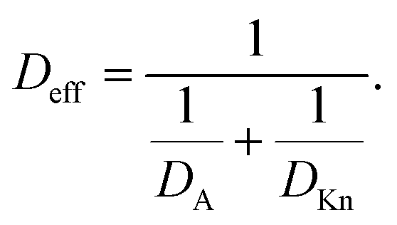
Unparalleled conformality is driving ever new applications for atomic layer deposition (ALD), a thin film growth method based on repeated self-terminating gas–solid reactions.1–3 ALD enables one to make conformal coatings on almost any desired inorganic substrate including high aspect ratio (HAR) structures such as microelectronics and powder media. Yet, tuning of the process parameters is often required to guarantee conformal coatings in HAR structures.Several types of feature-scale models have been used to simulate ALD growth in high aspect ratio (HAR) structures [e.g.Fig. 1(a)], as recently reviewed by Cremers et al.4 Analogously to a recent article on chemical vapor deposition,5 we classify these ALD models as ballistic line-of-sight (e.g. ref. 6–9), Monte Carlo (e.g. ref. 10–17) and diffusion–reaction models (e.g. ref. 18–23).§ While the heterogeneous gas–solid reactions responsible for ALD growth have been demonstrated in a great range of pressures from atmospheric to ultra-high vacuum,4,17,24 ALD processes often operate in a low vacuum of roughly 102 Pa range.3 Consequently, most feature-scale models for ALD have been developed for low-pressure conditions where the mean-free-path of the molecules λ is much higher than the limiting dimension of the feature h (Knudsen number Kn = λ/h ≫ 1).9,25 Here, molecules collide with the feature walls and not with other molecules in the gas phase, and the mass transport regime is referred to with varied names e.g. as (free) molecular flow, Knudsen flow, or Knudsen diffusion.4,19,26,27 Diffusion–reaction models based on Fick's law of diffusion can flexibly be used in free molecular flow (Kn ≫ 1) as well as in transition flow (Kn ≈ 1) and even under continuum flow (Kn ≪ 1) conditions,25,27,28 as the effective diffusion coefficient Deff (m−2 s−1) can be calculated from the gas-phase diffusion coefficient DA (m−2 s−1) and the Knudsen diffusion coefficient DKn (m−2 s−1).17,18,20 Also Monte Carlo methods have been used for regimes other than free molecular flow, by using the mean free path λ as a statistical parameter.11–13 Irrespective of the theoretical framework, all models reproduce the typical profiles of ideal ALD growth based on self-terminating (i.e., saturating and irreversible) reactions:3,29 constant film thickness followed by an abrupt decrease to zero, as illustrated in Fig. 1(b).
 | ||
| Fig. 1 Illustration of the ALD film in wide microchannel structures: (a) side and top views of the microchannel with length L and height H, containing a film with thickness s at the channel entrance (illustration intentionally not to scale). (b) Illustration of the different regions (I–IV) of a thickness profile superimposed on a thickness profile with different axes shown. The classifications of thickness profiles and the regions are as in ref. 40, except that here we use the term thickness profile instead of saturation profile. | ||
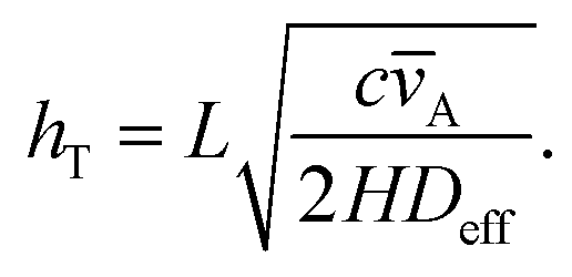
For ALD process modelling and reactor design, a useful description of the reaction kinetics is essential. Typically, the reaction kinetics of ALD processes are described in a simplified manner assuming irreversible single-site Langmuir adsorption and an associated (lumped) sticking coefficient.4,7,13,17,20,30 Experimental knowledge of sticking coefficients has been rather scarce until recently.4,7,8,11,12,30–34 The most straightforward way of analysing the kinetics is by interpreting film termination profiles measured in dedicated test structures or in a cross-flow reactor, where a steep film termination profile is generally associated with high reactivity.11,12,30,31,35,36 With a low sticking coefficient, the process can be in a reaction-limited regime, where no clear termination profile can be identified. Whether film growth is in a reaction-limited or diffusion-limited regime, can be estimated by the Thiele modulus hT (or α17,20,31 where α = hT2) which gives the ratio of the reaction rate to the diffusion rate.27 In the diffusion-limited regime, the value of Thiele modulus is much higher than one.27,37
Recently, microscopic lateral high-aspect-ratio (LHAR) test channels have emerged for thickness profile measurements.18,38–40 Such LHAR structures simplify conformality analysis: after ALD, the roof of the structure can be removed, exposing the film to detailed analysis.39–41 Furthermore, a slope method has been developed by Arts et al.31 to be used in conjunction with microscopic LHAR test channels, where the sticking coefficient c can be calculated from the slope [at a surface coverage θ (−) of 1/2] of the Type 1 normalized thickness profile40 [Fig. 1(b)] through a simple square root relationship.31 Here, a Type 1 normalized thickness profile40 refers to the normalized amount of growth (one for a saturated surface, or θ = 1) as the vertical axis and the dimensionless distance (distance divided by channel height) as the horizontal axis. This slope method was derived empirically from the diffusion–reaction model of Yanguas-Gil and Elam20 at free molecular flow conditions.
In this work, we have re-implemented the diffusion–reaction model by Ylilammi et al.18 and used it to simulate the evolution of ALD growth at various scenarios of kinetic and process parameters and diffusion regimes. We first describe the assumptions and equations behind the Ylilammi et al.18 diffusion-equation model. We then demonstrate how process parameters influence the ALD thickness profile by varying individual parameters at various diffusion regimes and channel filling levels. Finally, we compare the simulations of the Ylilammi et al.18 model with the Arts et al.31 slope method and discuss the likely reasons for the observed slight differences.
2. Description of the Ylilammi et al.18 diffusion–reaction model
For full details behind the model derivation, please see the article by Ylilammi et al.18 Here, core concepts are presented that are used in the current implementation. In some cases, somewhat expanded explanations are provided, to help the reader follow the model and connect it to other models on ALD.2.1. Basic ALD process and geometry assumptions
The Ylilammi et al.18 model was built to describe a typical ALD process, based on the use of inert gas for transporting the reactant from the source to the growth surface.3The considered high-aspect-ratio (HAR) geometry is a wide microchannel similar to the one in Fig. 1(a), where the height H (m) of the microchannel is the limiting dimension. The width W (m) of the microchannel is orders of magnitude larger than H, and the length L (m) is considered infinite (the channel end effects are not considered). While the model has been constructed with lateral HAR (LHAR) structures in mind,39,40 it is indifferent to the orientation of the structure and thus describes vertical trenches (and any other orientation) as well.
Typically, an ALD process has at least two reactants, often called Reactant A and Reactant B.3 In this model, one of the two reactions is assumed to limit the extent of film growth in the microchannel; typically, this is assumed to be the reaction of Reactant A. The partial pressure of Reactant A is denoted as pA (Pa). Reactant A is brought to the microchannel entrance at a partial pressure pA0.18 It is expected that the partial pressure of Reactant A behaves like a step function: during the reactant pulse, the pressure at the microchannel entrance is pA0, and otherwise it is zero.3,42 An inert carrier gas, denoted here with “I” (instead of the notation “B” used in the Ylilammi et al.18 article, to avoid confusion with Reactant B3), is used to aid the transport of Reactant A from the source to the surface. The inert gas has the same partial pressure pI (Pa) inside and outside of the microchannel. Inside the microchannel, pA decreases, as Reactant A is consumed in the adsorption (i.e., ALD) process. The time t from the beginning (t = 0) until the end of the exposure of Reactant A (t = t1) is considered; purge is excluded from this model. Thus, of the four typical steps in an ALD sequence,3 the current simulation concerns Step 1 (or Step 3) only.
2.2. Mass transport by diffusion and partial pressure of Reactant A
In the chosen geometry, the partial pressure of Reactant A can be considered constant in the y- and z-direction.18 The one-dimensional diffusion equation for the partial pressure of Reactant A pA (eqn (10) of Ylilammi et al.18) is: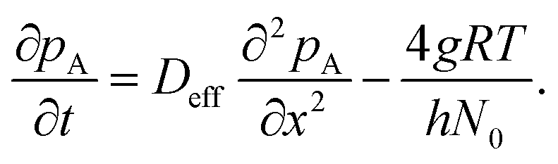 | (1) |
 | (2) |
 | (3) |
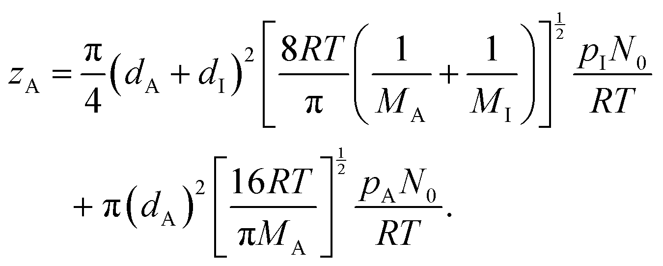
![[v with combining macron]](https://www.rsc.org/images/entities/i_char_0076_0304.gif) A (m s−1) and the collision rate of the Reactant A molecules in a mixture of A and B, zA (s−1) (eqn (3), Ylilammi et al.18):
A (m s−1) and the collision rate of the Reactant A molecules in a mixture of A and B, zA (s−1) (eqn (3), Ylilammi et al.18):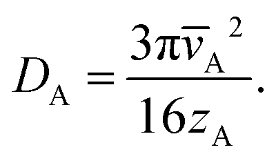 | (4) |
 | (5) |
 | (6) |
The Knudsen diffusion coefficient DKn depends on the microchannel's hydraulic diameter h, the temperature T, and the molar mass of Reactant A, MA (kg mol−1) (eqn (4) of Ylilammi et al.18):
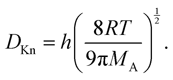 | (7) |
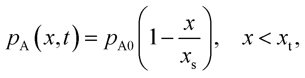
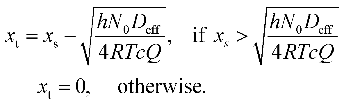
Instead of solving the differential equation for the partial pressure of Reactant A (eqn (10) of Ylilammi et al.18) numerically, Ylilammi et al.18 derived an approximate analytic solution of the diffusion equation, which is implemented in this work. With the approximate solution, the partial pressure of Reactant A pA can be analytically calculated for any position x and time t. In the part of the profile where the net adsorption rate g is approximately zero (x < xt, where t stands for “transition”), the partial pressure pA decreases linearly with x (eqn (18) of Ylilammi et al.18) (Fig. S1, ESI†):
 | (8) |
 | (9) |
 | (10) |
 | (11) |
 | (12) |
 | (13) |
 | (14) |
An illustration of how the partial pressure of Reactant A decreases inside the microchannel is shown in Fig. 2(a). Simulation conditions similar to those of Ylilammi et al.18 were used. Fig. 2(a) shows a similar trend as Fig. 2 in Ylilammi et al.,18 suggesting that the model was correctly re-implemented.
 | ||
| Fig. 2 Illustration of the simulated parameters inside the microchannel as a function of location and time: (a) partial pressure of Reactant A, and (b) surface coverage. The figures correspond to Fig. 2 and 3 of Ylilammi et al.,18 respectively. Parameters: c = 0.01, T = 500 K, pA0 = 100 Pa, MA = 0.0749 kg mol−1, dA = 5.91 × 10⁻¹⁰ m, pI = 300 Pa, MI = 0.028 kg mol−1, dI = 3.74 × 10⁻¹⁰ m, ρ = 4000 kg m−3, gpcsat = 1.06 × 10⁻¹⁰ m, K = 100 Pa−1, q = 5 nm−2, H = 0.5 μm, and W = 0.1 mm. | ||
2.3. Langmuir adsorption model and surface coverage
The model is built on the assumption of reversible single-site Langmuir adsorption describing the gas–solid reaction step in ALD:18| A + * ⇌ A*. | (15) |
The fraction of occupied adsorption sites is called the surface coverage and is denoted with θ (0 ≤ θ ≤ 1). The fraction of unoccupied or vacant adsorption sites is 1 − θ. The rate of adsorption per unit surface area fads (m−2 s−1) is proportional to the fraction of vacant sites, the probability that a collision leads to adsorption c, and the frequency of collisions pA, either as (eqn (11), Ylilammi et al.18):
 | (16) |
| fads = (1 − θ)cQpA. | (17) |
| fdes = θqPd. | (18) |
| g = fads − fdes. | (19) |
 | (20) |
During adsorption, the ALD reactions are generally not at equilibrium, and the surface coverage θ is a function of x and time t. In the model, the surface coverage is solved numerically from the rate equation describing the rate of change of the surface coverage with time (eqn (31), Ylilammi et al.18):
 | (21) |
An illustration of the surface coverage inside the microchannel is shown in Fig. 2(b). This figure shows a similar trend to Fig. 3 by Ylilammi et al.,18 indicating that the model has been correctly re-implemented.
2.4. Effect of cycles on film thickness and parameters such as narrowing of the channel
For each cycle, the surface coverage profile is calculated separately, as in eqn (21). The thickness increment caused by the surface coverage is (eqn (37), Ylilammi et al.18):| s(x) = θ(x)gpcsat. | (22) |
 | (23) |
In the Ylilammi et al. model,18 a simplification is made to assume that the free height of the microchannel H is decreased in each cycle by twice the GPC value, as the film grows both on the top and bottom of the microchannel (eqn (35), Ylilammi et al.18):
| H(N) = H(0) − 2Ngpcsat. | (24) |
3. Experimental
3.1. Model implementation in MATLAB®
In this work, ALD thickness profiles in LHAR with different conditions were simulated by implementing the Ylilammi et al.18 diffusion–reaction model (Model A). The sticking coefficients used for the simulation were compared with those back-extracted by the Arts et al.31 slope method, which is based on the Yanguas-Gil and Elam20 diffusion–reaction model (Model B). To discuss the reasons behind the observed differences, the partial pressure of Reactant A and surface coverage in LHAR were simulated also with Model B. | ||
| Fig. 3 Simplified algorithm for the simulation of thickness profiles with the re-implemented Ylilammi et al.18 diffusion–reaction model. | ||
The surface coverage profile θ(x,t) was computed by solving eqn (21) until the target pulse time was reached. The film thickness profile s(x) was obtained from eqn (22) while the thickness increment and the updated microchannel height were calculated from eqn (23) and (24), respectively. The previous procedure was repeated until the defined number of cycles (N) was achieved.
In this work, and in the work of Arts et al.31 reporting on the slope method,31 the coupled equations of the Yanguas-Gil and Elam model20 were solved assuming free molecular flow (i.e., Deff = DKn), using MATLAB's pdepe solver.43 This function solves a system of parabolic and elliptic partial differential equations with one spatial parameter (here, the distance x) and one time parameter t. For the implementation of Model B, the symmetry of the problem was set to 0, corresponding to slab geometry, and default tolerance values of 10−3 relative tolerance and 10−6 absolute tolerance were used. Analogous to the implementation of Model A, the parameters x and t were discretised using constant spacing. Finally, the initial conditions pA(x,0) = 0 and θ(x,0) = 0 were used, in combination with the boundary conditions pA(0, t) = pA0 and 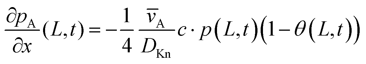 .20
.20
3.2. Simulation details
Simulations were made with MATLAB® scripts by varying an individual parameter while keeping other parameters constant. To extract the half-thickness penetration depth, the script chose the first point (xi,yi), where xi is equal to or smaller than the half-thickness penetration depth, and then chose another discretisation point (xi−1,yi−1), which was one point before (xi,yi). Once the two discretisation points were chosen, the half-thickness penetration depth and the slope at the half-thickness penetration depth were interpolated linearly between the two discretisation points (see Fig. S3, ESI†). The total number of discretisation points were selected so that the difference between those two discretisation points in the y-axis is less than or equal to 3% of the whole range.To compare the simulations made with the Ylilammi et al. model18 and the Yanguas-Gil and Elam model,20 and to back-extract the sticking coefficient by the slope method,31 we chose conditions with Kn ≥ 1009,25 and Thiele modulus hT > 1.27,37 The Knudsen number was calculated as (eqn (1), Cremers et al.4)
 | (25) |
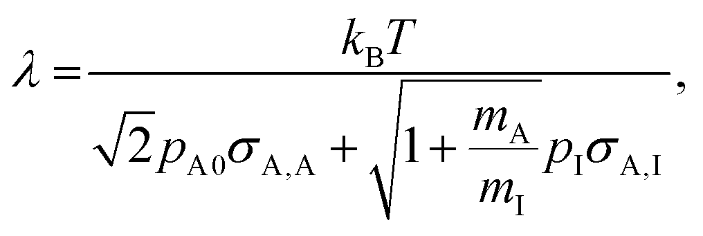
The mean free path λ was calculated as (eqn (3), Cremers et al.,4 and eqn (5.21),3 Chapman and Cowling44):
 | (26) |
 | (27) |
 | (28) |
The excess number γ, which refers to the amount of Reactant A existing per adsorption site in the LHAR structure,18 is calculated by using the following equation (eqn (6) Yanguas-Gil and Elam20):
 | (29) |
The sticking coefficient was back-extracted with the Arts et al.31 slope method derived from the Yanguas-Gil and Elam model20 as follows:
 | (30) |
![[x with combining tilde]](https://www.rsc.org/images/entities/i_char_0078_0303.gif) (−) is the dimensionless distance. In this work, the surface coverage θ was extracted from a Type 1 normalised thickness profile expressed as the normalised thickness s/(Ngpcsat) against the dimensionless distance . To back-extract the sticking coefficient the total number of discretisation points was selected so that the difference between the two discretisation points chosen in the y-axis was below 1% of the whole range.
(−) is the dimensionless distance. In this work, the surface coverage θ was extracted from a Type 1 normalised thickness profile expressed as the normalised thickness s/(Ngpcsat) against the dimensionless distance . To back-extract the sticking coefficient the total number of discretisation points was selected so that the difference between the two discretisation points chosen in the y-axis was below 1% of the whole range.
4. Results and discussion
4.1. ALD in microchannels: general trends with the baseline process
Trends in the evolution of conformality in the microchannels were initially investigated by defining a baseline process with parameters inspired by the experimental TMA–water process.18,39,40,45 For these simulations, the microchannel height H was chosen to be 500 nm, as typically used in microscopic PillarHallTM LHAR structures.18,31,40,46,47 The temperature was chosen to be 250 °C, which is in the typical temperature range of the TMA–water process.32 The partial pressure of Reactant A and the inert gas were chosen as 100 Pa and 500 Pa, respectively, and the Reactant A pulse length was chosen as 0.1 s; these conditions are similar to earlier reported experimental conditions.40,48 The adsorption density of the surface was set to 4 nm−2, which is in the range observed for the TMA–water process32,49,50 and in the range typical for ALD.42 The molar mass of Reactant A was set to an arbitrary value of 100 g mol−1, while that of the purge gas was typical for nitrogen (28 g mol−1). The diameters of Reactant A and the inert gas were 600 and 374 pm, respectively, as in the TMA–water simulation.18,40 The choice of H = 500 nm, combined with the pressure range used, resulted in the Knudsen number Kn for the baseline conditions being 7.6, which is in the transition flow regime (0.1 ≤ Kn ≤ 10).25 The varied parameters are presented in Table 1.| Parameter | Varied values | Effective Kn |
|---|---|---|
| a Other baseline parameters used: W = 10 mm, dA = 6 × 10⁻¹⁰ m, dI = 3.74 × 10⁻¹⁰ m, MI = 0.0280 kg mol−1, bfilm = 1, bA = 1, and M = 0.050 kg mol−1. In all the examples used in this study, Thiele modulus27,37hT > 1 (for otherwise baseline conditions with varied sticking coefficients of 1, 0.1, 0.01, 0.001, and 0.0001, hT was 898, 284, 90, 28, and 9, respectively; the effective diffusion coefficient was used for the Thiele modulus calculation). | ||
| p A0 (Pa) | 50, 100, 200, 400, 800 | 8.2, 7.6, 6.5, 5.0, 3.5 |
| t 1 (s) | 0.05, 0.1, 0.2, 0.4, 0.8 | 7.6 |
| M A (kg mol−1) | 0.0250, 0.050, 0.100, 0.200, 0.400 | 10.7, 9.2, 7.6, 5.9, 4.5 |
| ρ (kg m−3) | 2500, 3000, 3500, 4000, 4500 | 7.6 |
| q (nm−2) | 1, 2, 4, 8, 10 | 7.6 |
| P d (s−1) | 0.01, 0.1, 1, 10, 100 | 7.6 |
| c (−) | 0.0001, 0.001, 0.01, 0.1, 1 | 7.6 |
| T (°C) | 100, 150, 200, 250, 300 | 5.4, 6.1, 6.8, 7.6, 8.3 |
| p I (Pa) | 0.1, 250, 500, 750, 1000 | 45.2, 12.9, 7.6, 5.3, 4.1 |
| H (μm) | 0.1, 0.2, 0.5, 1, 2, 2.5, 4 | 37.8, 18.9, 7.6, 3.8, 1.9, 1.5, 0.9 |
| N (−) | 5, 10, 20, 50, 100, 250, 500 | 7.6 |
The thickness profiles simulated with varied parameters are shown in Fig. 4(a)–(i). Panels (a) and (b), respectively, show that an increase in the partial pressure of Reactant A, pA, and the pulse time of Reactant A, t1, both significantly increase the penetration depth of the film. This result is as expected: the product of pA and t1 is the dose (Pa s) that defines the penetration depth at free molecular flow conditions (half-thickness penetration depth  ).20,26,31 Panel (c) shows the effect of varying the molar mass of Reactant A, MA. The penetration depth of the film is higher when the molecules are lighter. This is consistent with the fact that the diffusion of light molecules is faster than that of heavy molecules (eqn (4) and (7)). Panel (d) illustrates the effect of varying the mass density of the grown MyZx material, ρ. The lower the density, the higher the grown thickness (note that the penetration depth is not affected). With a lower density, one unit of MyZx takes up a larger space, so a constant adsorption density q leads to a larger film volume and therefore a larger thickness (eqn (12)). (Note: the thickness-based GPC is not constant in such a case.3) Panel (e) illustrates the effect of the adsorption density, q (i.e. GPC expressed as the areal number density) on the thickness profile. With other parameters constant, the adsorption density has a strong influence on the growth. This is not surprising, since gpcsat is the core parameter describing an ALD process.1–3,29,32 The higher the gpcsat, the higher the film thickness in the saturated region but the lower the penetration depth. This observation is consistent with and explains recent experimental findings where a higher gpcsat resulted in a lower penetration depth.40,45,51 Panel (f) shows how varying the desorption probability, Pd, affects the simulation (the Ylilammi et al.18 model allows reversible reactions). High values of desorption probability affect the shape of the thickness profile especially in Region II, before the Region III of fast decrease (for the regions, see Fig. 1). Panel (g) illustrates the effect of varying the sticking coefficient of Reactant A, c. The sticking coefficient strongly affects the shape of the resulting thickness profile, as already known from earlier simulations made for the diffusion-limited regime.12,30,31 Varying the process temperature T and the inert gas pressure pI has a minor effect on the penetration depth, as seen from panels (h) and (i), respectively.
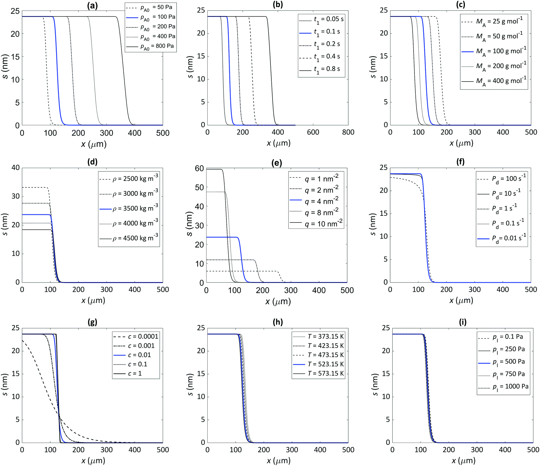 | ||
| Fig. 4 Illustration of the effect of varying individual parameters on the thickness profile in microchannels, simulated with the Ylilammi et al. model18 re-implemented in this work. The parameter values used in the simulation are presented in Table 1. Simulations with the baseline values are shown as a solid blue line. The effect of the (a) initial partial pressure of the Reactant A, pA0, (b) pulse length of Reactant A, t1, (c) molecular mass of Reactant A, MA, (d) film density, ρ, (e) adsorption density, q (i.e. GPC expressed as areal number density), (f) desorption probability, Pd, (g) (lumped) sticking coefficient, c, (h) ALD process temperature, T, and (i) inert gas pressure, pI. Note that the image of panel (b) has a larger distance in the horizontal axis than the other images. | ||
Earlier works have shown the importance of the sticking coefficient,11,12,30 as well as the components defining the reactant dose18,22,25– i.e., reaction time and reactant pressure – on the characteristics of the thickness profile. Simulations made in this work for a typical baseline process resembling the archetypical TMA–water ALD process demonstrated that the process parameters such as the molar mass of the reactant, the adsorption density (derived from the GPC), and the mass density of the film also influence the detailed features of the thickness profile.
4.2. Effect of filling of the microchannel on the simulated thickness profile
When a film grows into a microchannel, in each ALD cycle, the channel gets narrower from both sides by twice the value of the GPC (eqn (24)). The film thickness that completely fills the microchannel is thus half of the microchannel height H. Although an experimental ALD thickness profile can be measured after any number of cycles, the expected shape will depend on the number of ALD cycles, as shown in ref. 40.How much can a microchannel be filled so that a “fingerprint” ALD thickness profile can be measured, whose shape and characteristics are not yet affected by the already grown film? From this fingerprint thickness profile, it is possible to extract the sticking coefficient with the simple slope method.31 Previously, a preferable filling of less than 10% was proposed.40 Here, the effect of the channel filling on the resulting thickness profile was simulated, using the same baseline conditions as in the previous section (Table 1), and varying either the microchannel height H or the number of cycles N.
The results of the simulation series illustrating the effect of channel filling are shown in Fig. 5. In the thickness profiles of panels (a) and (b), the expected features are observed: with a larger microchannel height, the penetration depth increases, and with an increasing number of cycles, the film thickness increases. The scaled thickness profiles of panels (c) and (d) reveal finer trends. With a constant film thickness and varied microchannel height (c), the half-thickness penetration depth 50% (−) first increases with increasing microchannel height, and then starts to decrease [panel (e)]. With a constant microchannel height and a varying film thickness of panel (d), the scaled thickness profiles simulated for the smallest cycle numbers (5 to 20) approximately overlap, but already for channel filling of a few percent, the penetration depth starts to decrease with channel filling [panel (e)]. Numerical information regarding the half-thickness penetration depth 50% and the slope at this point is presented in Table S1 (ESI†).
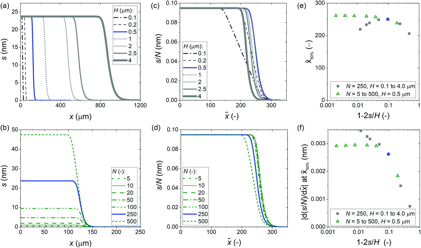 | ||
| Fig. 5 Illustration of the channel filling effect on the ALD thickness profile in wide microchannels. The parameters used in the simulations are given in Table 1. Baseline simulation results are marked in blue. (a) Thickness profiles simulated with a constant number of cycles of 250 and a varied channel height. (b) Thickness profiles simulated with a constant channel height of 500 nm and a varied number of cycles. (c) The scaled thickness profile from the data of panel (a). (d) The scaled thickness profile from the data of panel (b). (e) The half-thickness penetration depth of the scaled thickness profile as a function of the channel filling fraction, for the data presented in panels (c) and (d). (f) The slope at half-thickness penetration depth as a function of the channel filling fraction (1 − 2s/H), from the data presented in panels (a/c) and (b/d). | ||
The slope at half-thickness penetration depth is shown for both simulation series in Fig. 5(f). For the series where the number of cycles was varied, the slope settles to a constant value (ca. −0.0029) for the smallest amounts of channel filling, as expected. The case where the channel height was varied, shows a different trend: with decreasing channel filling, after a knee, the absolute value of the slope increases again. Table S1 (ESI†) shows the Knudsen number Kn calculated in each case. The knee point occurs at Kn = 8 which is in the transition flow regime.25 Because of the increasing channel height, the Knudsen number decreases with decreasing channel filling (see Fig. S5, ESI†). The reason for the somewhat unexpected trend of the increasing slope with increasing channel height (and decreasing channel filling) was the transition from free molecular flow towards transition flow (Kn < 10), where gas-phase collisions make the diffusion coefficient smaller.
From the simulations made to explore the effect of channel filling, the following can be concluded. (i) To be in the region where the thickness profile is independent of the number of cycles, the channel filling should not exceed a few percent. (ii) The flow regime affects the thickness profile, including the numerical characteristics of the half-thickness penetration depth and the slope at half-thickness penetration depth. To measure a fingerprint thickness profile for an ALD process, the flow condition must be free molecular flow (Kn ≫ 1). To check whether this is the case, the mean free path of the molecules should be calculated (eqn (26)) and compared to the limiting dimension of the feature (eqn (25)).
4.3. Comparison of thickness profile trends at free molecular flow and transition flow regimes
The simulations in the previous sections revealed that (i) the thickness profile characteristics depend on the flow regime and (ii) the thickness of the grown film affects the characteristics of the thickness profile already from a filling of a few percent.To compare the trends of the ALD thickness profile in different flow regimes in a well-defined way, we varied individual process parameters to make ALD thickness profiles in free molecular flow (Kn ≫ 1) and transition flow (Kn ≈ 1) conditions.25,27,28 A comparison was made with a single cycle, so that the channel filling does not influence the trends of the thickness profile. Both the scaled thickness profile and the Type 1 normalized thickness profile were used as a basis for comparison. The scaled thickness profile is the most informative thickness profile for an ALD process, and the Type 1 normalized thickness profile is the basis of the slope method.31 The thickness profiles are presented in Fig. S6–S9 (ESI†). For each case, the trends in the half-thickness penetration depth 50% (−) and the absolute value of the slope at 50% were analysed. The numerical values are shown in Fig. S10–S15 (ESI†).
The qualitative thickness profile trends in the free molecular flow and transition flow regimes are summarised in Table 2. In the free molecular flow, the half-thickness penetration depth and the absolute value of the slope remained constant with varying channel heights, as expected. In the transition flow, the penetration depth decreased, and the absolute value of the slope increased with increasing channel heights, most likely resulting from gas-phase collisions. An increase in the reactant partial pressure and pulse time highly increased the penetration depth in both free molecular flow and transition flow, as expected. The desorption probability did not affect the penetration depth and the absolute value of the slope in either flow regime. The penetration depth decreased slightly with the increasing process temperature in both flow regimes.
| Simulation parameter (increases) | Kn ≫ 1 | Kn ≈ 1 | ||||
|---|---|---|---|---|---|---|
|
50%
|
|
|
50%
|
|
|
|
| (−) | (nm) | (−) | (−) | (nm) | (−) | |
a The parameter values used for the centre point in the free molecular flow regime were: W = 10 mm, H = 5 × 10⁻² μm, N = 1, T = 573.15 K, t1 = 0.1 s, pA0 = 50 Pa, MA = 0.1 kg mol−1, dA = 6.0 × 10⁻¹⁰ m, MI = 0.028 kg mol−1, dI = 4.0 × 10⁻¹⁰ m, pI = 250 Pa, q = 4 nm−2, ρ = 3500 kg m−3, M = 0.050 kg mol−1, Pd = 0.01 s−1, and c = 0.01. The parameter values used for the centre point in transition flow regimes were: W = 10 mm, H = 0.5 μm, N = 1, T = 573.15 K, t1 = 0.1 s, pA0 = 500 Pa, MA = 0.1 kg mol−1, dA = 6.0 × 10⁻¹⁰ m, MI = 0.028 kg mol−1, dI = 4.0 × 10⁻¹⁰ m, pI = 2500 Pa, q = 4 nm−2, ρ = 3500 kg m−3, M = 0.050 kg mol−1, Pd = 0.01 s−1, and c = 0.01.
b The total pressure p was increased by increasing the partial pressure of the inert gas pI from 0.5 to 250 Pa with a constant reactant partial pressure pA0 of 50 Pa in free molecular flow and by increasing the partial pressure of the inert gas pI from 625 to 10![[thin space (1/6-em)]](https://www.rsc.org/images/entities/char_2009.gif) 000 Pa with constant reactant partial pressure pA0 of 500 Pa in transition flow.
c The initial partial pressure of Reactant A was varied from 1 to 100 Pa, with a constant partial pressure of the inert gas pI of 250 Pa in free molecular flow. The initial partial pressure of Reactant A was varied from 100 to 1000 Pa, with a constant partial pressure of the inert gas pI of 2500 Pa in transition flow. 000 Pa with constant reactant partial pressure pA0 of 500 Pa in transition flow.
c The initial partial pressure of Reactant A was varied from 1 to 100 Pa, with a constant partial pressure of the inert gas pI of 250 Pa in free molecular flow. The initial partial pressure of Reactant A was varied from 100 to 1000 Pa, with a constant partial pressure of the inert gas pI of 2500 Pa in transition flow.
|
||||||
| Channel height (H) | — | — | — | ↓ | ↑ | ↑ |
| Initial partial pressure of the ALD Reactant A (pA0) | ↑↑ | — | — | ↑↑ | — | — |
| Reactant pulse time (t1) | ↑↑↑ | — | — | ↑↑↑ | — | — |
| Sticking coefficient (c) | ↑ | ↑↑↑ | ↑↑↑ | ↑ | ↑↑↑ | ↑↑↑ |
| Desorption probability (Pd) | — | — | — | — | — | — |
| Adsorption density (q) | ↓ ↓ ↓ | ↑↑ | — | ↓ ↓ ↓ | ↑↑ | — |
| Temperature (T) | ↓ | — | — | ↓ | — | — |
| Total pressure (p)b | — | — | — | ↓ | ↑ | ↑ |
| Fraction of reactant pressure of total pressure (pA0/p)c | ↑↑ | — | — | ↑↑ | — | — |
| Molecular mass of the ALD reactant (MA) | ↓ | — | — | ↓ | ↑ | ↑ |
| Molecular mass of the carrier gas (MI) | — | — | — | ↑ | ↓ | ↓ |
| Size of the reactant molecule (dA) | — | — | — | — | ↑ | ↑ |
| Density of the grown material (ρ) | — | ↓ | — | — | ↓ | — |


Some process parameters affected the trends of the thickness profile differently in different flow regimes. The molar mass of Reactant A did not affect the absolute value of the slope in free molecular flow while the absolute value of the slope slightly increased with increasing molar mass in the transition flow. The inert gas influenced the thickness profile differently in free molecular flow and transition flow. The inert gas parameters did not affect the penetration depth or the slope in the free molecular flow regime, as expected. In the transition flow regime, the half-thickness penetration depth slightly decreased with increasing pressure and decreasing molar mass of the inert gas. The absolute value of the slope slightly increased with the increasing pressure and decreasing molar mass of inert gas. The absolute value of the slope in the transition flow regime slightly increased with increasing reactant size, while the reactant size did not affect the thickness profile in the free molecular flow regime.
In general, the scaled thickness profile showed the same trends as the Type 1 normalized thickness profile. However, there were two exceptions. With increasing adsorption density q, the absolute value of the slope of the scaled thickness profile markedly increased, while that of the Type 1 normalized thickness profile remained constant. With increasing density of the grown film ρ, the absolute value of the slope of the scaled thickness profile slightly decreased, while that of the Type 1 normalized thickness profile remained constant.
4.4. Comparison of the simulations with different models
Sticking coefficients used for simulations of Model A18 were compared to those back-extracted from their thickness profiles with the slope method31 (eqn (30)). Different scenarios with varying process temperatures, molar masses, and sticking coefficients were tested, with parameters defined so that the mass transport was always in the free molecular flow regime (Kn ≥ 100), and the excess number γ was ≪1,36 as it is where the slope method31 is valid. Fig. 6(a) shows that when Kn ≥ 100, the effective diffusion coefficient Deff becomes practically identical to the Knudsen diffusion coefficient DKn. Note that the comparison was made at conditions where the number of ALD cycles was one. If a larger number of cycles were used and part of the microchannel got filled by the growing film, the slope and penetration depth would have decreased. This channel filling would affect the extracted sticking coefficient and, thus, the comparison. | ||
| Fig. 6 (a) Diffusion coefficients (eqn (2), (4), and (7)) against the Knudsen number (Kn). Knudsen numbers were varied by varying pA0 from 1 to 20480 Pa (the pA0 to pI ratio was 1 to 5). A comparison of the sticking coefficient values back-extracted using the slope method31 (marked with open triangles) with the set values (marked with open circles) used for simulation, implementing the Ylilammi et al. model18 with different (b) ALD process temperatures, T, (c) molar masses of Reactant A, MA, and (d) sticking coefficients. The parameter values used, if not otherwise stated: W = 10 mm, H = 0.1 μm, N = 1, T = 523.15 K, t1 = 2 s, pA0 = 10 Pa, MA = 0.1 kg mol−1, dA = 6.0 × 10⁻¹⁰ m, MI = 0.028 kg mol−1, dI = 3.74 × 10⁻¹⁰ m, pI = 50 Pa, q = 4 nm−2, ρ = 3500 kg m−3, M = 0.050 kg mol−1, Pd = 10−5 s−1, and c = 0.01. | ||
Fig. 6 panels (b)–(d) show the sticking coefficients back-extracted by the slope method31 compared to set values. Table 3 lists the parameter values used for simulations and the back-extracted sticking coefficients. Fig. S16 (ESI†) shows Type 1 normalized thickness profiles used for the back extraction of (lumped) sticking coefficients. While the order of magnitude is the same, the back-extracted sticking coefficients are systematically ca. 25% higher than the set values (see Table 3). Therefore, it seems that the slope method31 can be used to back-extract sticking coefficients from thickness profiles simulated with the current implementation of the Ylilammi et al.18 model by simply applying a correction factor.
| Series | T (K) | M A (kg mol−1) | c (−) | Kn (−) |
|
c ext (−) | c ext/c (−) |
|---|---|---|---|---|---|---|---|
|
a Parameters used, if not otherwise stated: W = 10 mm, H = 0.1 μm, T = 523.15 K, N = 1, t1 = 2 s, pA0 = 10 Pa, MA = 0.1 kg mol−1, dA = 6.0 × 10⁻¹⁰ m, MI = 0.028 kg mol−1, dI = 3.74 × 10⁻¹⁰ m, pI = 50 Pa, q = 4 nm−2, ρ = 3500 kg m−3, M = 0.050 kg mol−1, Pd = 10−5 s−1, and c = 0.01. To satisfy the criteria of a difference between the two discretisation points in the y-axis below 1% of the whole range, 5000 discretisation points were used in the simulations with varied molar mass of Reactant A and process temperature while in the simulation with varied sticking coefficient 30000 discretisation points were used.
|
|||||||
| ALD process temperature | 323.15 | 0.1 | 0.01 | 233 | 0.0300 | 0.0125 | 1.25 |
| 423.15 | 0.1 | 0.01 | 305 | 0.0301 | 0.0126 | 1.26 | |
| 523.15 | 0.1 | 0.01 | 378 | 0.0300 | 0.0125 | 1.25 | |
| 623.15 | 0.1 | 0.01 | 450 | 0.0300 | 0.0125 | 1.25 | |
| 723.15 | 0.1 | 0.01 | 522 | 0.0300 | 0.0125 | 1.25 | |
| Molar mass of Reactant A | 523.15 | 0.025 | 0.01 | 537 | 0.0301 | 0.0126 | 1.26 |
| 523.15 | 0.05 | 0.01 | 462 | 0.0300 | 0.0125 | 1.25 | |
| 523.15 | 0.1 | 0.01 | 378 | 0.0300 | 0.0125 | 1.25 | |
| 523.15 | 0.2 | 0.01 | 295 | 0.0300 | 0.0125 | 1.25 | |
| 523.15 | 0.4 | 0.01 | 223 | 0.0300 | 0.0125 | 1.25 | |
| Sticking coefficient | 523.15 | 0.1 | 0.0001 | 378 | 0.0030 | 0.000126 | 1.26 |
| 523.15 | 0.1 | 0.001 | 378 | 0.0095 | 0.00125 | 1.25 | |
| 523.15 | 0.1 | 0.01 | 378 | 0.0300 | 0.0125 | 1.25 | |
| 523.15 | 0.1 | 0.1 | 378 | 0.0951 | 0.126 | 1.26 | |
| 523.15 | 0.1 | 1 | 378 | 0.3004 | 1.25 | 1.25 | |

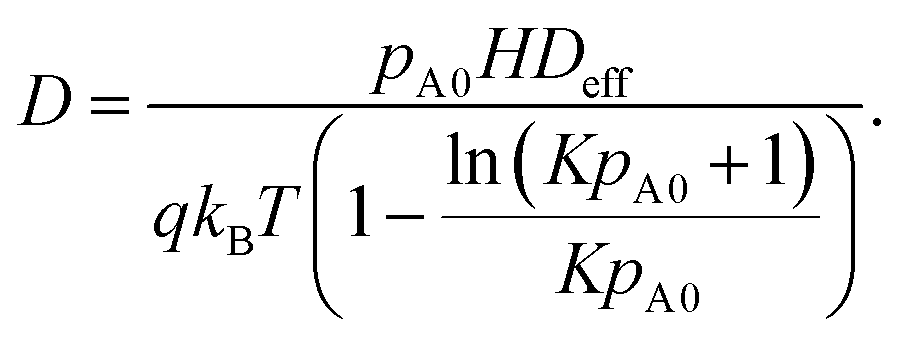
To analyse possible sources of differences in the sticking coefficient values, we compared the partial pressure of Reactant A along the microchannels simulated with the Ylilammi et al.18 model (Model A) and the Yanguas-Gil and Elam20 model (Model B); Model B forms the basis of the slope method.31Fig. 7 shows the surface coverage and partial pressure simulated with the above two models against the dimensionless distance. Fig. 7(b) shows observable differences in partial pressures and coverage profiles especially in Region III of the thickness profile [regions are shown in Fig. 1(b)], which is the adsorption front where the thickness rapidly decreases.40 A difference compared to Model B is expected, since the Ylilammi et al.18 model introduced a simplified analytical approximation to the partial pressure (eqn (8) and (9)) (Fig. S1 and S17, ESI†). We conclude that the more rapid drop of pressure pA at the adsorption front simulated by Model A caused a higher absolute slope value extracted at half-thickness penetration depth, and thus a slightly higher back-extracted sticking coefficient compared to the set value. Despite this limitation, Model A is still useful to predict the effect of various process conditions on thickness profile, as shown in this work.
 | ||
| Fig. 7 (a) Surface coverage θ and partial pressure of Reactant A pA within the dimensionless distance simulated by model A (ref. 18) and model B (ref. 20). (b) Details of the area marked with a square in panel (a). Parameter values used: c = 0.01, t1 = 2 s, T = 523.15 K, pA0 = 10 Pa, N = 1, MA = 0.1 kg mol−1, dA = 6.0 × 10⁻¹⁰ m, pI = 50 Pa, MI = 0.028 kg mol−1, dI = 3.74 × 10⁻¹⁰ m, ρ = 3500 kg m−3, M = 0.050 kg mol−1, Pd = 10−5 s−1, q = 4 nm−2, H = 0.5 μm, and W = 10 mm. | ||
5. Conclusions and outlook
This work re-implemented the Ylilammi et al.18 diffusion–reaction model for ALD conformality analysis through thickness profile simulation and used that model to explore trends in the thickness profile inside wide microchannels in different diffusion regimes encountered in reality.A series of simulations were made to explore the effect on thickness profile characteristics at free molecular flow and transition flow conditions of kinetic and process parameters, such as temperature, (lumped) sticking coefficient, molar mass of the ALD reactant, the reactant's exposure time and pressure, total pressure, density of the grown material, and GPC of the ALD process. Increasing the molar mass and the GPC, for example, resulted in a decreasing penetration depth into the LHAR channel. Trends with the parameter changed depending on the flow regime. To obtain an ALD measurable or a “fingerprint” characteristic for a specific ALD process the following conditions should be met: (i) free molecular flow should be the governing mass transport regime, (ii) the channel filling should remain below 5%, and (iii) the scaled thickness profile should be presented, with the dimensionless distance on the horizontal axis and the thickness divided by cycles on the vertical axis. From such a fingerprint thickness profile, the characteristic GPC is evident, and the kinetic information can be extracted by various means.
The simulations were compared with the recent slope method by back-extracting the sticking coefficient from the ALD thickness profiles at free molecular flow conditions. The slope method gave systematically somewhat higher sticking coefficient values than input values. The difference is most likely related to how, to speed up simulations, the partial pressure of Reactant A inside the channel is analytically approximated in the re-implemented model.
For reactor modelling, kinetic information of real ALD processes is needed. Recent advances have made it possible to measure experimental thickness profiles, which contain the necessary kinetic information, without the need of time-consuming post-preparation of HAR samples. Several theoretical models have been developed to extract (lumped) sticking coefficient parameters from such experimental data. This work has shown that (i) to obtain experimental data for kinetic experiments, detailed knowledge of the experimental conditions, especially pressure, is important, to choose a suitable model for the parameter extraction (most models are based on free molecular flow assumption). Furthermore, (ii) there are differences between the models. The same data fitted with different models may give different results for the extracted fundamental kinetic growth parameters, as the details of the model implementation may affect the results.
For speedy development of the fundamental understanding of ALD processes, and to compare models with each other and with data, it would be advantageous if the scientific ALD community could publish experimental thickness profiles as Open Data and models as Open Code. First such initiatives have already been made: an Open Data community has been initiated in Zenodo.org,52 and the first ALD simulation code has been published in Github.53 The simulation codes of this work are to be published accordingly.
Author contributions
The manuscript was compiled by J. Y. The re-implementation of the Ylilammi et al.18 diffusion–reaction model (Model A) through the MATLAB scripts was done by E. V. and described by J. A. V. Most of the thickness profiles were simulated based on Model A by J. Y., E. V., and J. A. V. Some of the thickness profiles were simulated by re-implementing the Yanguas-Gil and Elam20 model (Model B) by K. A., and the re-implementation of Model B was described by K. A. The sticking coefficient was back-extracted using the slope method31 and compared to the set values for the Model A simulation by J. Y. The comparison of the simulation results from Model A with Model B was done by J. Y. and K. A. The work was initiated and supervised by R. L. P. All authors discussed the results and contributed to the final manuscript.Funding sources
The work was financially supported by the Academy of Finland (COOLCAT consortium, decision no. 329978 and ALDI consortium, decision no. 331082) and by Prof. Puurunen's starting grant at Aalto University.List of symbols
| b | Number of metal atoms in a reactant molecule in the Ylilammi et al.18 model (−) |
| c | Sticking coefficient (−) |
| c ext | Sticking coefficient back-extracted with the slope method31 (−) |
| D | Apparent longitudinal diffusion coefficient in the Ylilammi et al.18 model (m2 s−1) |
| D A | Gas-phase diffusion coefficient of Reactant A (m2 s−1) |
| D eff | Effective diffusion coefficient (m2 s−1) |
| D Kn | Knudsen diffusion coefficient (m2 s−1) |
| d A | Hard-sphere diameter of molecule A (m) |
| d I | Hard-sphere diameter of the inert gas molecule (m) |
| f ads | Adsorption rate (m−2 s−1) |
| f des | Desorption rate (m−2 s−1) |
| g | Net adsorption rate (m−2 s−1) |
| gpcsat | Saturation growth per cycle, thickness-based, in the Ylilammi et al.18 model (m) |
| h | Hydraulic diameter of the channel (m) |
| H | Height of the channel (m) |
| h T | Thiele modulus (−)27,37 |
| K | Adsorption equilibrium constant in the Ylilammi et al.18 model (Pa−1) |
| Kn | Knudsen number (−) |
| k B | Boltzmann constant (m2 kg s−2 K−1) |
| L | Length of the channel (m) |
| M | Molar mass of the deposited film material (kg mol−1) |
| M A | Molar mass of Reactant A (kg mol−1) |
| M I | Molar mass of the inert gas I (kg mol−1) (MB in Ylilammi et al.18) |
| N | Number of ALD cycles |
| n A | Particle concentration of Reactant A (m−3) |
| N 0 | Avogadro's constant (mol−1) |
| p | Total pressure (pA0 + pI) (Pa) |
| p A | Partial pressure of Reactant A (Pa) |
| p A0 | Initial partial pressure of Reactant A (Pa) |
| p I | Partial pressure of the inert gas I (Pa) |
| p At | Partial pressure of Reactant A at xt (Pa) |
| P d | Desorption probability in unit time in the Ylilammi et al.18 model (s−1) |
| q | Adsorption density of metal M atoms in the growth of film of the MyZx material (m−2) (i.e. GPC expressed as areal number density) |
| Q | Collision rate with surface at unit pressure in the Ylilammi et al.18 model (m−2 s−1 Pa−1) |
| r i | Hard-sphere radius of molecule i (m) |
| R | Gas constant (J K−1 mol−1) |
| s | Film thickness in the Ylilammi et al.18 model (m) |
| S | Surface area of the microchannel (m2) |
| t | Time (s) |
| t 1 | Length of the Reactant A pulse (as Step 1 of a typical ALD cycle3) (s) |
| T | Temperature (K) |
| v | Velocity of gas front in the Ylilammi et al.18 model (m s−1) |
| V | Volume of the microchannel (m3) |
|
A
| Average speed of molecules A (m s−1) |
| W | Width of the channel (m) |
| x | Distance from the channel entrance (m) |
| x 50% | Half-thickness penetration depth (m) (expressed as xp in Ylilammi et al.18) |
|
| Dimensionless distance into the channel, x/H (−) |
|
50%
| Half-thickness penetration depth (−) |
| x s | Distance where the extrapolated linear part of the reactant pressure is zero in the Ylilammi et al.18 model (m) |
| x t | Distance of the linear part of the reactant pressure distribution in the Ylilammi et al.18 model (m) |
| z A | Collision frequency of Reactant A with other gas molecules in a gas mixture of Reactant A + inert gas I (s−1) |
| θ | Surface coverage (−), 0 ≤ θ ≤ 1 |
| ρ | Mass density of the deposited film (kg m−3) |
| λ | Mean free path (m) |
| σ i,j | Collision cross section between the molecules i and j (m2) |
| γ | Excess number in the Yanguas-Gil and Elam20 model (−) |
Conflicts of interest
There are no conflicts of interest to declare.Acknowledgements
The authors thank Angel Yanguas-Gil, J. Ruud van Ommen, Ville Alopaeus, Ville Vuorinen, Gizem Ersavas Isitman and Jänis Järvilehto for the useful discussions on ALD modelling. Part of the results presented of this work were presented at the international ALD conferences, organised virtually by the American Vacuum Society (AVS) in 2020 and 2021. The MATLAB simulation codes created in this work will be made openly available. A community for open data related to the experimental and simulated ALD thickness profiles is available at https://zenodo.org/communities/ald-saturation-profile-open-data/.References
- T. Suntola, Atomic layer epitaxy, Mater. Sci. Rep., 1989, 4, 261–312 CrossRef CAS.
- S. M. George, Atomic Layer Deposition: An Overview, Chem. Rev., 2010, 110, 111–131 CrossRef CAS PubMed.
- J. R. van Ommen, A. Goulas and R. L. Puurunen, Atomic layer deposition, Kirk-Othmer Encyclopedia of Chemical Technology, John Wiley & Sons, Inc, 2021 Search PubMed.
- V. Cremers, R. L. Puurunen and J. Dendooven, Conformality in atomic layer deposition: current status overview of analysis and modelling, Appl. Phys. Rev., 2019, 6, 021302 Search PubMed.
- N. Cheimarios, G. Kokkoris and A. G. Boudouvis, Multiscale Modeling in Chemical Vapor Deposition Processes: Models and Methodologies, Archives Comput. Methods Eng., 2021, 28, 637–672 CrossRef.
- A. Yanguas-Gil and J. W. Elam, A Markov chain approach to simulate atomic layer deposition chemistry and transport inside nanostructured substrates, Theor. Chem. Acc., 2014, 133, 1465 Search PubMed.
- R. A. Adomaitis, A ballistic transport and surface reaction model for simulating atomic layer deposition processes in high-aspect-ratio nanopores, Chem. Vap. Deposition, 2011, 17, 353–365 CrossRef CAS.
- J.-Y. Kim, J.-H. Kim, J.-H. Ahn, P.-K. Park and S.-W. Kang, Applicability of Step-Coverage Modeling to TiO2 Thin Films in Atomic Layer Deposition, J. Electrochem. Soc., 2007, 154, H1008 CrossRef CAS.
- M. K. Gobbert, V. Prasad and T. S. Cale, Predictive modeling of atomic layer deposition on the feature scale, Thin Solid Films, 2002, 410, 129–141 CrossRef CAS.
- J. W. Elam, D. Routkevitch, P. P. Mardilovich and S. M. George, Conformal coating on ultrahigh-aspect-ratio nanopores of anodic alumina by atomic layer deposition, Chem. Mater., 2003, 15, 3507–3517 CrossRef CAS.
- M. C. Schwille, T. Schössler, J. Barth, M. Knaut, F. Schön, A. Höchst, M. Oettel and J. W. Bartha, Experimental and simulation approach for process optimization of atomic layer deposited thin films in high aspect ratio 3D structures, J. Vac. Sci. Technol., A, 2017, 35, 01B118 CrossRef.
- M. Rose and J. W. Bartha, Method to determine the sticking coefficient of precursor molecules in atomic layer deposition, Appl. Surf. Sci., 2009, 255, 6620–6623 CrossRef CAS.
- V. Cremers, F. Geenen, C. Detavernier and J. Dendooven, Monte Carlo simulations of atomic layer deposition on 3D large surface area structures: Required precursor exposure for pillar- versus hole-type structures, J. Vac. Sci. Technol., A, 2017, 35, 01B115 CrossRef.
- H. C. M. Knoops, E. Langereis, M. C. M. van de Sanden and W. M. M. Kessels, Conformality of Plasma-Assisted ALD: Physical Processes and Modeling, J. Electrochem. Soc., 2010, 157, G241–G249 CrossRef CAS.
- J. Dendooven, D. Deduytsche, J. Musschoot, R. L. Vanmeirhaeghe and C. Detavernier, Conformality of Al2O3 and AlN Deposited by Plasma-Enhanced Atomic Layer Deposition, J. Electrochem. Soc., 2010, 157, G111–G116 CrossRef CAS.
- H. Shimizu, K. Sakoda, T. Momose, M. Koshi and Y. Shimogaki, Hot-wire-assisted atomic layer deposition of a high quality cobalt film using cobaltocene: Elementary reaction analysis on NHx radical formation, J. Vac. Sci. Technol., A, 2012, 30, 01A144 CrossRef.
- P. Poodt, A. Mameli, J. Schulpen, W. M. M. Kessels and F. Roozeboom, Effect of reactor pressure on the conformal coating inside porous substrates by atomic layer deposition, J. Vac. Sci. Technol., A, 2017, 35, 021502 CrossRef.
- M. Ylilammi, O. M. E. Ylivaara and R. L. Puurunen, Modeling growth kinetics of thin films made by atomic layer deposition in lateral high-aspect-ratio structures, J. Appl. Phys., 2018, 123, 205301 CrossRef.
- H. Y. Lee, C. J. An, S. J. Piao, D. Y. Ahn, M. T. Kim and Y. S. Min, Shrinking core model for Knudsen diffusion-limited atomic layer deposition on a nanoporous monolith with an ultrahigh aspect ratio, J. Phys. Chem. C, 2010, 114, 18601–18606 CrossRef CAS.
- A. Yanguas-Gil and J. W. Elam, Self-limited reaction-diffusion in nanostructured substrates: Surface coverage dynamics and analytic approximations to ALD saturation times, Chem. Vap. Deposition, 2012, 18, 46–52 CrossRef CAS.
- A. J. Gayle, Z. J. Berquist, Y. Chen, A. J. Hill, J. Y. Hoffman, A. R. Bielinski, A. Lenert and N. P. Dasgupta, Tunable Atomic Layer Deposition into Ultra-High-Aspect-Ratio (>60000:1) Aerogel Monoliths Enabled by Transport Modeling, Chem. Mater., 2021, 33, 5572–5583 CrossRef CAS.
- W. Z. Fang, Y. Q. Tang, C. Ban, Q. Kang, R. Qiao and W. Q. Tao, Atomic layer deposition in porous electrodes: A pore-scale modeling study, Chem. Eng. J., 2019, 378, 122099 CrossRef CAS.
- T. Keuter, N. H. Menzler, G. Mauer, F. Vondahlen, R. Vaßen and H. P. Buchkremer, Modeling precursor diffusion and reaction of atomic layer deposition in porous structures, J. Vac. Sci. Technol., A, 2015, 33, 01A104 CrossRef.
- H. van Bui, F. Grillo and J. R. van Ommen, Atomic and molecular layer deposition: off the beaten track, Chem. Commun., 2017, 53, 45–71 RSC.
- S. Roy, R. Raju, H. F. Chuang, B. A. Cruden and M. Meyyappan, Modeling gas flow through microchannels and nanopores, J. Appl. Phys., 2003, 93, 4870–4879 CrossRef CAS.
- R. G. Gordon, D. Hausmann, E. Kim and J. Shepard, A kinetic model for step coverage by atomic layer deposition in narrow holes or trenches, Chem. Vap. Deposition, 2003, 9, 73–78 CrossRef CAS.
- A. Yanguas-Gil, Growth and Transport in Nanostructured Materials: Reactive Transport in PVD, CVD, and ALD, Springer, 2017 Search PubMed.
- Z. Li, K. Cao, X. Li and R. Chen, Computational fluid dynamics modeling of spatial atomic layer deposition on microgroove substrates, Int. J. Heat Mass Transfer, 2021, 181, 121854 CrossRef CAS.
- H. H. Sønsteby, A. Yanguas-Gil and J. W. Elam, Consistency and reproducibility in atomic layer deposition, J. Vac. Sci. Technol., A, 2020, 38, 020804 CrossRef.
- J. Dendooven, D. Deduytsche, J. Musschoot, R. L. Vanmeirhaeghe and C. Detavernier, Modeling the Conformality of Atomic Layer Deposition: The Effect of Sticking Probability, J. Electrochem. Soc., 2009, 156, P63–P67 CrossRef CAS.
- K. Arts, V. Vandalon, R. L. Puurunen, M. Utriainen, F. Gao, W. M. M. Kessels and H. C. M. Knoops, Sticking probabilities of H2O and Al(CH3)3 during atomic layer deposition of Al2O3 extracted from their impact on film conformality, J. Vac. Sci. Technol., A, 2019, 37, 030908 CrossRef.
- R. L. Puurunen, Surface chemistry of atomic layer deposition: a case study for the trimethylaluminum/water process, J. Appl. Phys., 2005, 97, 121301 CrossRef.
- M. Rose, J. W. Bartha and I. Endler, Temperature dependence of the sticking coefficient in atomic layer deposition, Appl. Surf. Sci., 2010, 256, 3778–3782 CrossRef CAS.
- M. C. Schwille, T. Schössler, F. Schön, M. Oettel and J. W. Bartha, Temperature dependence of the sticking coefficients of bis-diethyl aminosilane and trimethylaluminum in atomic layer deposition, J. Vac. Sci. Technol., A, 2017, 35, 01B119 CrossRef.
- J. Aarik and H. Siimon, Characterization of adsorption in flow type atomic layer epitaxy reactor, Appl. Surf. Sci., 1994, 81, 281–287 CrossRef CAS.
- A. Yanguas-Gil and J. W. Elam, Simple model for atomic layer deposition precursor reaction and transport in a viscous-flow tubular reactor, J. Vac. Sci. Technol., A, 2012, 30, 01A159 CrossRef.
- E. W. Thiele, Relation between catalytic activity and size of particle, Ind. Eng. Chem., 1939, 31, 916–920 CrossRef CAS.
- PillarHall, http://www.pillarhall.com/, (accessed August 23, 2021).
- F. Gao, S. Arpiainen and R. L. Puurunen, Microscopic silicon-based lateral high-aspect-ratio structures for thin film conformality analysis, J. Vac. Sci. Technol., A, 2015, 33, 010601 CrossRef.
- J. Yim, O. M. E. Ylivaara, M. Ylilammi, V. Korpelainen, E. Haimi, E. Verkama, M. Utriainen and R. L. Puurunen, Saturation profile based conformality analysis for atomic layer deposition: Aluminum oxide in lateral high-aspect-ratio channels, Phys. Chem. Chem. Phys., 2020, 22, 23107–23120 RSC.
- E. Haimi, O. M. E. Ylivaara, J. Yim and R. L. Puurunen, Saturation profile measurement of atomic layer deposited film by X-ray microanalysis on lateral high-aspect-ratio structure, Appl. Surf. Sci. Adv., 2021, 5, 100102 CrossRef.
- T. Blomberg, (Invited) Unit Steps of an ALD Half-Cycle, ECS Trans., 2013, 58, 3–18 CrossRef.
- pdepe, https://www.mathworks.com/help/matlab/ref/pdepe.html, (accessed August 23, 2021).
- S. Chapman and T. G. Cowling, The Mathematical Theory of Non-Uniform Gases: An Account of the Kinetic Theory of Viscosity, Thermal Conduction and Diffusion in Gases, Cambridge University Press, 1970 Search PubMed.
- R. L. Puurunen and F. Gao, Influence of ALD temperature on thin film conformality: Investigation with microscopic lateral high-aspect-ratio structures, 14th International Baltic Conference on Atomic Layer Deposition (BALD), St. Petersburg (IEEE), 2016, pp. 20–24.
- K. Arts, J. H. Deijkers, T. Faraz, R. L. Puurunen, W. M. M. E. Kessels and H. C. M. Knoops, Evidence for low-energy ions influencing plasma-assisted atomic layer deposition of SiO2: Impact on the growth per cycle and wet etch rate, Appl. Phys. Lett., 2020, 117, 031602 CrossRef CAS.
- K. Arts, M. Utriainen, R. L. Puurunen, W. M. M. E. Kessels and H. C. M. Knoops, Film Conformality and Extracted Recombination Probabilities of O Atoms during Plasma-assisted Atomic Layer Deposition of SiO2, TiO2, Al2O3, and HfO2, J. Phys. Chem. C, 2019, 123, 27030–27035 CrossRef CAS.
- O. M. E. Ylivaara, L. Kilpi, X. Liu, S. Sintonen, S. Ali, M. Laitinen, J. Julin, E. Haimi, T. Sajavaara, H. Lipsanen, S.-P. Hannula, H. Ronkainen and R. L. Puurunen, Aluminum oxide/titanium dioxide nanolaminates grown by atomic layer deposition: Growth and mechanical properties, J. Vac. Sci. Technol., A, 2017, 35, 01B105 CrossRef.
- R. L. Puurunen, Correlation between the growth-per-cycle and the surface hydroxyl group concentration in the atomic layer deposition of aluminum oxide from trimethylaluminum and water, Appl. Surf. Sci., 2005, 245, 6–10 CrossRef CAS.
- O. M. E. Ylivaara, X. Liu, L. Kilpi, J. Lyytinen, D. Schneider, M. Laitinen, J. Julin, S. Ali, S. Sintonen, M. Berdova, E. Haimi, T. Sajavaara, H. Ronkainen, H. Lipsanen, J. Koskinen, S.-P. Hannula and R. L. Puurunen, Aluminum oxide from trimethylaluminum and water by atomic layer deposition: The temperature dependence of residual stress, elastic modulus, hardness and adhesion, Thin Solid Films, 2014, 552, 124–135 CrossRef CAS.
- M. Mattinen, J. Hämäläinen, F. Gao, P. Jalkanen, K. Mizohata, J. Räisänen, R. L. Puurunen, M. Ritala and M. Leskelä, Nucleation and Conformality of Iridium and Iridium Oxide Thin Films Grown by Atomic Layer Deposition, Langmuir, 2016, 32, 10559–10569 CrossRef CAS PubMed.
- ALD saturation profile – open data, https://zenodo.org/communities/ald-saturation-profile-open-data/, (accessed July 14, 2021).
- A. Yanguas-Gil and J. W. Elam, machball, https://github.com/aldsim/machball, (accessed July 14, 2021).
- P. Atkins and J. de Paula, Atkins' Physical Chemistry, Oxford University Press, 8th edn, 2006 Search PubMed.
Footnotes |
| † Electronic supplementary information (ESI) available. See DOI: 10.1039/d1cp04758b |
| ‡ These authors contributed equally. |
| § Diffusion-reaction models relying on Fick's laws of diffusion are in the ALD literature sometimes somewhat confusingly referred to as “continuum” models;4,31,36 in this work the term is dedicated to continuum flow conditions where the mean free path of molecules λ (m) is orders of magnitude smaller than the limiting feature dimension h (m) (Knudsen number Kn = λ/h ≤ 10−3).25 |
| ¶ Note that eqn (1) of Ylilammi et al.18 for calculating the collision frequency contains an error:40 both terms on the right side of eqn (1) of ref. 18 have been multiplied by Avogadro's number for eqn (6) of this work. |
| || Earlier report re-implemented the Ylilammi et al.18 model to simulate the growth of aluminium oxide from trimethylaluminium (TMA) and water in wide microchannels.40 |
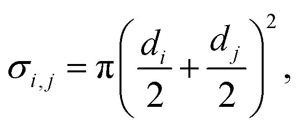
| ** Note that eqn (4) of Cremers et al.4 for calculating the collision cross section contains an error: instead of taking the sum of squares (ri2 + rj2),4 one should take the square of the sum (ri + rj)2, where ri (m) is the radius of molecule i. For the correct equation, see e.g. eqn (24.3b) of Atkins and De Paula.54 |
| This journal is © the Owner Societies 2022 |