Modelling quenching mechanisms of disordered molecular systems in the presence of molecular aggregates†
Received
17th September 2021
, Accepted 11th December 2021
First published on 13th December 2021
Abstract
Exciton density dynamics recorded in time-resolved spectroscopic measurements is a useful tool to recover information on energy transfer (ET) processes that can occur at different timescales, up to the ultrafast regime. Macroscopic models of exciton density decays, involving both direct Förster-like ET and diffusion mechanisms for exciton–exciton annihilation, are largely used to fit time-resolved experimental data but generally neglect contributions from molecular aggregates that can work as quenching species. In this work, we introduce a macroscopic model that includes contributions from molecular aggregate quenchers in a disordered molecular system. As an exemplifying case, we considered a homogenous distribution of rhodamine B dyes embedded in organic nanoparticles to set the initial parameters of the proposed model. The influence of such model parameters is systematically analysed, showing that the presence of molecular aggregate quenchers can be monitored by evaluating the exciton density long time decays. We showed that the proposed model can be applied to molecular systems with ultrafast decays, and we anticipated that it could be used in future studies for global fitting of experimental data with potential support from first-principles simulations.
Introduction
The theoretical modelling of exciton density dynamics allows shedding light on the photophysical processes occurring within photoactive materials, such as those employed in the development of artificial light-harvesting systems and organic light emitting diodes. Typical materials of interest are those based on conjugated polymers in the solid phase,1–4 where structural defects localize the excited states into small portions of the polymer chain acting as independent dyes, but several studies have been performed on aggregates in the solid phase,5,6 thin solid films of organic dyes7,8 and on the so-called host–guest systems, where organic dyes are spatially distributed within polymeric hosts in the form of films9,10 or nanoparticles.11,12 If dyes are weakly interacting, one can assume that excitons are localized on individual dyes and thus are able to move by dye distribution. This exciton mobility can be described by invoking an incoherent energy transfer (ET) hopping mechanism, which can be successfully described by the Förster theory of the ET.13,14 In the Förster model, the timescale governing the donor–acceptor ET is strictly dictated by the radiative (or fluorescence) lifetime of the donor molecule. Typical lifetimes for fluorophores range within the nanosecond scale, but several ETs have been experimentally observed to occur also on the picosecond2,15 and ultrafast femtosecond16 timescales.
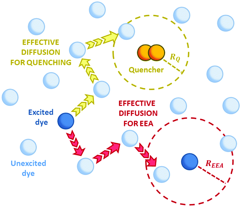
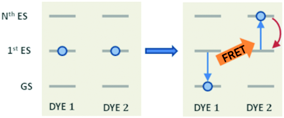
Other than the exciton mobility, the ET can be responsible for quenching mechanisms which remove excitations from the system. A quenching process driven by ET is the so-called exciton–exciton annihilation (EEA), which leads to a loss of excitations from the system due to the interaction between the excited states of two molecular dyes in spatial proximity. As shown in Fig. 1, the EEA occurs when an excited dye transfers its excitation energy to another excited dye, promoting it to a higher excited state while returning to its ground state. The lifetime of higher excited states is usually very small due to the fast non-radiative internal conversion processes which are likely to relax back the dye to its first excited state. Since the higher excited state can be rapidly depopulated via non-radiative mechanisms, the whole process describes a fast loss of excitation from the system.
 |
| | Fig. 1 The mechanism for exciton–exction annihilation (EEA). The excitation is transferred between two excited dyes (DYES 1 and 2), leading to an excited state absorption (to the Nth excited state) in one dye (DYE 2) and to a relaxation to the ground state in the other one (DYE 1). The Nth high-lying state is expected to rapidly decay non-radiatively (red arrow) to the first excited state, leading to the annihilation of one excitation (i.e. that of DYE 1). | |
The time evolution of the exciton density, which can also occur in an ultrafast time scale,17 is generally studied by means of transient absorption2,3,5–9,17 or photoluminescence decay10,18,19 measurements. The recorded, time-resolved signal is proportional to the time-dependent exciton density within the sample, and the proportionality constant is usually recovered by determining the number of absorbing dyes, i.e. their excitation probability under illumination by the light pulse used. In photoluminescence decay experiments, straightforward evidence for the presence of EEA is the acceleration of the fluorescence signal decay upon increasing the excitation power: since powerful irradiation excites a higher number of dyes, excited dyes become closer in space thereby increasing their annihilation probability. Still, the decay of the excitation density can also be affected by other competing quenching phenomena, such as the ET to non-fluorescent aggregates of dyes that is often neglected, while the role of molecular aggregation in the photophysical properties of optical systems is attracting increasing attention. For instance, the effect of the aggregation has been extensively studied in the application of rhodamine B based dyes employed in the building of artificial light harvesting nanosystems.11,20 Rhodamine B aggregates are known to be fluorescence quenchers21,22 and it has been demonstrated that the use of bulky hydrophobic counterions efficiently prevent aggregation.23,24 Previous theoretical investigations suggested that such a quenching mechanism could be due to the fact that rhodamine B dimers (with H-type aggregation) feature dark charge-transfer excited states very close in energy to the bright states, allowing for internal conversion processes that provide suitable paths for non-radiative decays.22
Reliable theoretical simulations of the fluorescence decay acceleration in the presence of EEA can thus provide essential information on the spatial distribution of molecular excitations and on the concomitant role of molecular aggregation in photoactive materials. The theoretical simulation of the time evolution of the exciton density in the presence of EEA could be derived through a microscopic description based on the quantum master equation formalism,25 which gives the time evolution of the population of each individual dye, but this level of theory requires a deep knowledge of the dye distribution, in particular of the distances between dyes and their relative orientation. In fact, such an approach has been applied to conjugated polymers for which simplified but reliable spatial models are available,26–28 but for disordered systems detailed information about the structure cannot be straightforwardly achieved. A simpler level of description invokes for a macroscopic description of the exciton density by strictly assuming a homogeneous distribution of dyes. Exclusively in this framework, the exciton density n(t) (quantifying the number of excited dyes per volume unit) in the presence of EEA can be described using the following equation:
| | 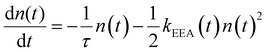 | (1) |
Here, the first term describes the decay due to the excited state dye lifetime, with lifetime
τ comprising both radiative and non-radiative processes, while the second term describes the decay due to EEA. As shown in
Fig. 2, three different models have been developed to express the rate constant
kEEA.
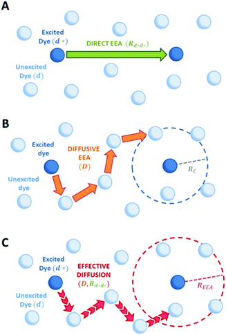 |
| | Fig. 2 Schematic representation of possible EEA mechanisms. (A) The direct mechanism follows the Förster theory and the ET is governed by the Förster radius  . (B) The diffusion mechanism involves a sequence of energy hops moving from the excited dye through the unexcited ones described by a diffusion coefficient D, while the EEA is assumed to take place when the exciton enters the contact sphere defined by the contact radius RC. (C) The model of Gösele et al. (in the predominant direct mechanism regime as proposed in ref. 8) describes the combined effect of both direct and diffusive mechanisms as an effective diffusive mechanism driven by the usual diffusion coefficient D but governed by a new contact radius REEA, which in turns depends on both the Förster radius Rd*d* and D. . (B) The diffusion mechanism involves a sequence of energy hops moving from the excited dye through the unexcited ones described by a diffusion coefficient D, while the EEA is assumed to take place when the exciton enters the contact sphere defined by the contact radius RC. (C) The model of Gösele et al. (in the predominant direct mechanism regime as proposed in ref. 8) describes the combined effect of both direct and diffusive mechanisms as an effective diffusive mechanism driven by the usual diffusion coefficient D but governed by a new contact radius REEA, which in turns depends on both the Förster radius Rd*d* and D. | |
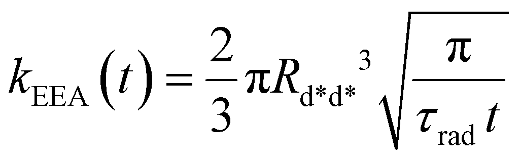
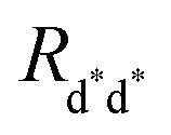
In the “direct mechanism” model, the EEA is assumed to occur as described by the Förster ET theory (Fig. 2A), and the rate constant takes the form originally derived by Förster13 for a generic donor–acceptor pair:
| | 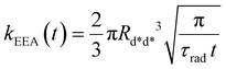 | (2) |
where
Rd*d* is the Förster radius related to the ET between two excited dyes and
τrad is the fluorescence lifetime of the dye. The
t−1/2 time dependence indicates the fact that excitations in close proximity annihilate firstly, thus reducing with time the probability of having annihilation events.
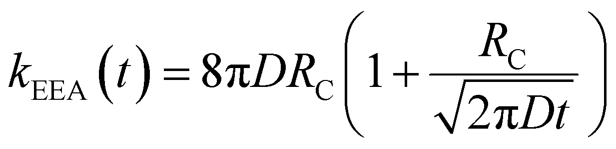
In the “diffusive mechanism” model, the excitations are allowed to diffuse through dyes, and the EEA is assumed to take place when two excitations reach a certain contact radius RC (Fig. 2B). The rate constant takes the form derived for the generic problem of a diffusing particle captured by an immobile capturing center:29
| | 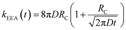 | (3) |
Here,
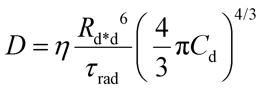
D is the diffusion coefficient describing the excitation mobility within the dye network. If we consider excitations moving in the dye network through a Förster hopping mechanism, the diffusion coefficient may be expressed as
30–33| |  | (4) |
where
Rd*d is the Förster radius related to the ET between an excited and a relaxed dye,
Cd is the dye concentration and
η = 0.43 is a factor accounting for the homogeneous distribution of dyes. The capability of
eqn (4) to correctly estimate the diffusion coefficient has been analysed in detail by Colby
et al.,
10 showing that its successful application could be compromised by several conditions such as the dye aggregation, the breakdown of the dipole–dipole interaction to describe the electronic coupling or the anomalous diffusion driven by energetic and orientational disorder. In this work, we will assume a framework in which the expression for the diffusion coefficient given by
eqn (4) is valid and the dye aggregation contribution can be treated separately (as the aggregates, acting as quenchers, will not be directly involved in the diffusion processes).
Eqn (4), in fact, allows for an interesting parametrization of the diffusion-related phenomena by simply introducing the additional Förster radius
Rd*q.
Gösele et al.34–37 derived equations for the rate constant considering both direct and diffusive mechanisms, as depicted in Fig. 2A and B, and their results have been re-obtained starting from a more sophisticated model by Jang et al.38 They distinguish two different regimes, having one among the diffusive or the direct ET mechanisms as predominant. For each regime, they also consider two limiting temporal scales: the short-time scale, where only one mechanism is assumed to rapidly start, and the long-time scale, where a stationary regime is assumed, i.e. the probability of having a decay due to both mechanisms is considered constant in time. The authors proposed that an approximate form for the global rate constants (one for each regime) should be obtained by simply summing the expressions for the two temporal scales. In the predominant diffusion regime, at short times only the diffusive mechanism is assumed to occur, and the global rate equation takes the same form of the pure diffusive case, eqn (3). In this work we will focus on the predominant direct ET regime (see Fig. 2C), which has been already suggested for simulations of the exciton density decays.9 In this regime, the diffusion is assumed not to have started yet at short times, and the rate constant kshortEEA(t) becomes the same as that of the Förster model in eqn (2), while at long times the rate constant takes the form
| | 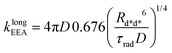 | (5) |
It is worth noting that although the direct mechanism is predominant, for the rate constant a dependence on the diffusion coefficient exists. The global rate constant is finally calculated as
| | | kEEA(t) ≈ kshortEEA(t) + klongEEA | (6) |
which can be rewritten in a compact form as
| | 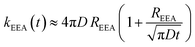 | (7) |
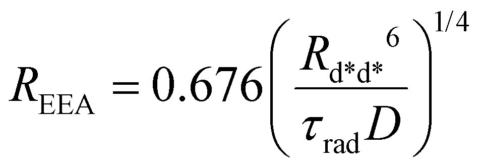
where a new “annihilation radius”
REEA has been introduced
| | 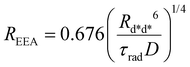 | (8) |
Since the expression obtained for the rate constant has the same form as the diffusive mechanism one,
eqn (3), we can consider the combination of the two processes as a new “effective diffusion” process, with a new contact distance equal to the annihilation radius (see
Fig. 2C).
As mentioned above, it could be the case where EEA is not the only process responsible for the decay of the excitation density: if the system contains intruder quenching species (such as non-fluorescent aggregates of dyes), the ET from excited dyes to these molecular quenchers will act as a new channel for wasting excitations. Once the excitation energy has been transferred to quenchers, they likely do not relax instantaneously but rather feature a non-radiative lifetime, which implies that an excited quencher density evolving in time has to be considered. In this work, the excitation density time-evolution of a photoactive system involving both the EEA and the dye-to-quencher ET phenomena (with dyes’ aggregates as quenchers) is phenomenologically modelled based on the model of Gösele et al. in a regime where the direct ET is the predominant effect. We report a detailed analysis of the effects of the presence of a small amount of quenchers and of the influence of all model parameters used to simulate the exciton density decays in disordered molecular systems. In order to describe the applicability of the model to a realistic system, we consider as a hypothetical case of study the distribution of the alkyl rhodamine B dye with bulky counterions within the organic nanoparticles presented in ref. 11, from which we take some parameters, such as the dye's fluorescence lifetime and concentration. We finally discuss the usefulness of the model for the global fitting of experimental data and its applicability, which should stimulate future developments to obtain model parameters from first-principles simulations.
Results and discussion
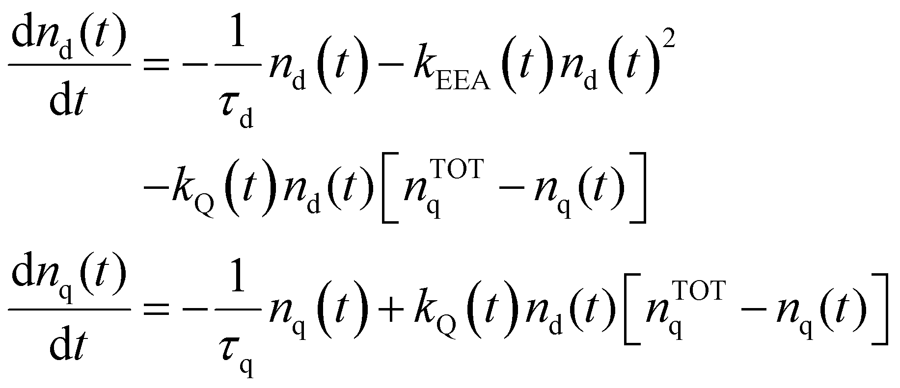
The time evolution of the excitation densities for dyes nd(t) and quenchers nq(t) (we assume no triplet state population) is described using the following system of coupled equations:| | 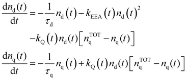 | (9) |
where nTOTq − nq(t) is the density of relaxed quenchers expressed in terms of the total concentration of quenchers nTOTq, and τd and τq being the total lifetimes of the dye and quencher, respectively (accounting for both non-radiative and radiative processes in the case of the dye).
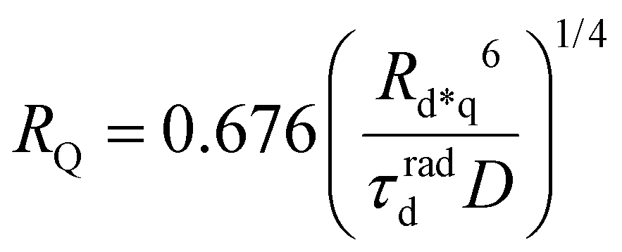
The ET processes considered in our model are depicted in Fig. 3. The rate constants for the EEA are described by eqn (7) and (8) with a diffusion coefficient given by eqn (4), and similar expressions are considered also for the dye–quencher ET:
| | 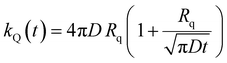 | (10) |
| |  | (11) |
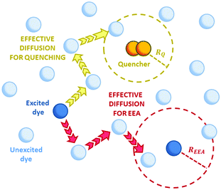 |
| | Fig. 3 The two possible mechanisms for the exciton loss in the presence of both EEA and quenching species (such as dimers in the case of rhodamine B) described by the Gösele model in the predominant direct mechanism regime. The new introduced contact radii REEA and Rq depend on the Förster radii Rd*d* and Rd*q respectively, and also depend on the same diffusion coefficient D. | |
In the following, the analysis of parameters affecting the numerical solution of eqn (9) is reported by assuming a small amount of quenching species within the dye distribution. We consider as a reference dye rhodamine B, having a radiative lifetime τradd = 4.24 ns (corresponding to the measured value for the 0.1% loaded nanoparticles in ref. 20) with a concentration of CTOTd = 0.13 dyes per nm3 (corresponding to the 30% loaded nanoparticles in ref. 20). We initially assume the quencher to not exceed 1% of the dye concentration, thus simulating a typical experimental situation in which a residual aggregation persists in the system despite the efforts made to prevent it. We neglect, for simplicity, the possibility of having non-radiative contributions to the lifetime of both the dye and quencher. Eqn (9) has to be solved imposing certain initial conditions, that is the exciton density at the time zero, nd(0): we consider that immediately after the light pulse 7% of the total dyes are excited (a population value falling in the typical experimental range in ref. 9), while we assume that no quenchers are initially excited. This assumption is based on the fact that a small amount of aggregates is present in the sample (we generally consider <1% of CTOTd) and likely their absorption maximum is shifted from that of isolated dyes since, to work as quenchers, a strong electronic coupling has to be present among the monomeric units. The effect of varying the initial values of the exciton density simulates the typical acceleration of the exciton density decay upon a power light increase in experiments (an example is provided in the ESI,† see Fig. S1 in Section S.1).
The following analysis aims at highlighting the various effects of the parameters entering our model, emphasizing those features that could allow a straightforward identification of the presence of intruder quenching species. We also explored how much such analysis could depend on the initially chosen values for dye/quencher lifetimes and concentrations, showing the adaptability of our tools to various molecular systems with ET processes occurring at different time scales, from nanoseconds to ultrafast.
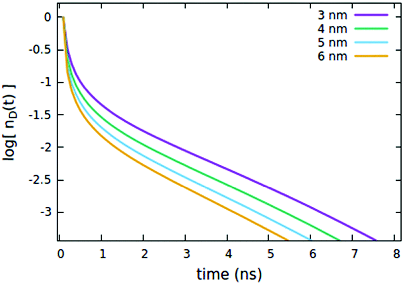
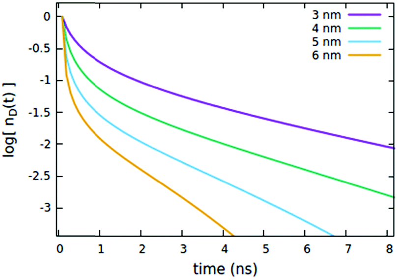
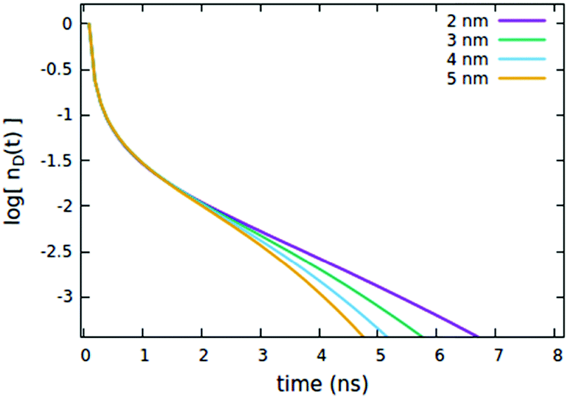
First, we consider the effects of the Förster radii Rd*d and Rd*d*, governing the exciton mobility through diffusion (influencing both diffusive EEA and diffusive ET to the quenchers) and the direct EEA, respectively. Typical values for Förster radii are up to 8 nm,39 thus we decided to test values within the 3–6 nm range. To highlight the effect of the two EEA processes, the Rd*q radius governing the dye–quencher ET and the quencher concentration Cq are set to small values, i.e. 2 nm and 0.25% of CTOTd respectively. From Fig. 4 it is clear that Rd*d* has an influence only on the decays at short time, with the initial decay accelerating upon increasing the radius while leaving the long time evolution unaltered. This result indicates that the EEA events, following the direct mechanism, start immediately after the light pulse and becomes less probable with time, as the spatially closed excitations are depleted through annihilation.
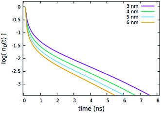 |
| | Fig. 4 Effect of the Rd*d* radius governing the direct EEA mechanism on the (normalized) exciton density decay. Fixed parameters are Rd*d = 5 nm; Rd*q = 2 nm; τq = 4 ns; Cq = 0.25% of CTOTd; nd(0) = 7% of CTOTd. | |
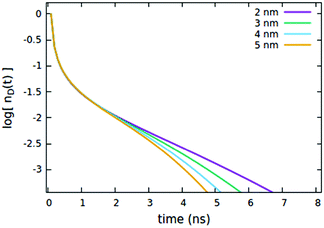
The influence of the Rd*d radius is quite different from that of Rd*d*, as clearly shown in Fig. 5. Differently from the radius governing the direct EEA, it affects both the short and the long time evolution. While the influence on the short times is similar to Rd*d*, here also the long-time decays accelerate upon increasing the radius.
 |
| | Fig. 5 Effect of the Rd*d radius governing both EEA and quenching diffusive mechanisms on the (normalized) exciton density decay. Fixed parameters are Rd*d* = 4 nm; Rd*q = 2 nm; τq = 4 ns; Cq = 0.25% of CTOTd; nd(0) = 7% of CTOTd. | |
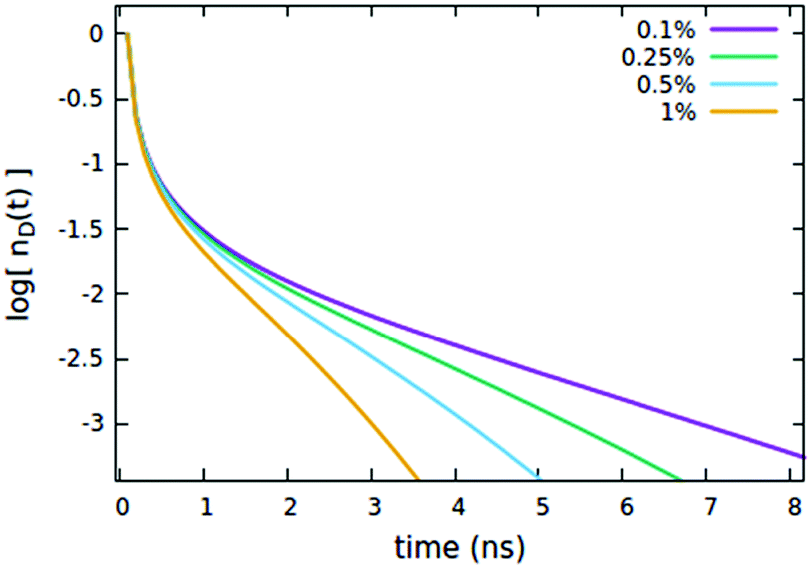
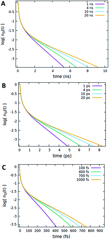
We now consider the effect of the parameters related to the quencher species, i.e. its concentration Cq, Förster radius Rd*q and radiative lifetime τradd, as reported in Fig. 6, 7 and 8A, respectively. It is evident that when the quencher is present in a small amount, its influence can affect the long time evolution only, since a few quencher molecules are very far from the majority of excited dyes and then a certain time has to pass to allow excitations to diffuse towards them. Since this specific (isolated) effect on the long-time evolution cannot be obtained by varying the parameters related to the EEA only, it represents a straightforward signature for the presence of intruder quenching species. Notably, all the trends described above involving an initial amount of excited dyes (nd(0) = 7% of the CTOTd), i.e.Fig. 2–7, are preserved when such an initial (fixed) parameter is significantly increased (see Fig. S2–S7 in Section S.2 of the ESI,† for trends with nd(0) = 25% of the CTOTd).
 |
| | Fig. 6 Effect of the Rd*q radius governing the direct quenching mechanism on the (normalized) exciton density decay. Fixed parameters are Rd*d* = 4 nm; Rd*d = 5 nm; τq = 4 ns; Cq = 0.25% of CTOTd; nd(0) = 7% of CTOTd. | |
 |
| | Fig. 7 Effect of the quencher concentration Cq (expressed as % of CTOTd) on the (normalized) exciton density decay. Fixed parameters are Rd*d = 5 nm; Rd*d* = 4 nm; Rd*q = 2 nm; τq = 4 ns, Cq = 0.25% of CTOTd; nd(0) = 7% of CTOTd. | |
 |
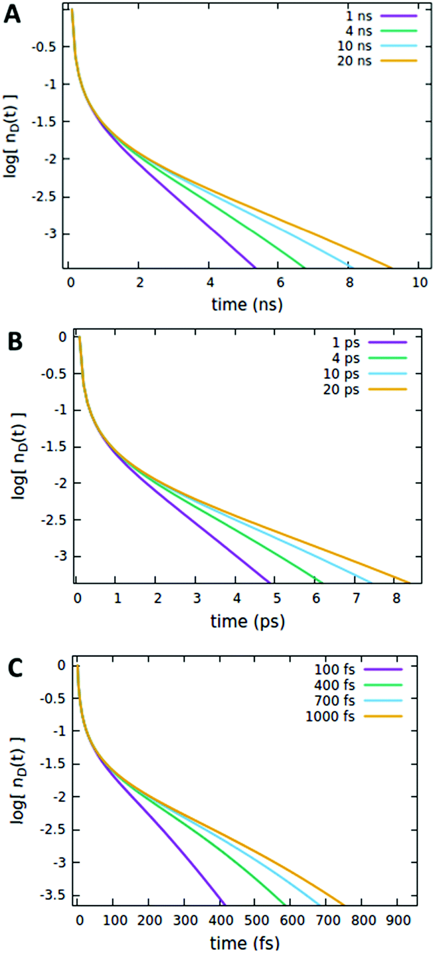
| | Fig. 8 The effect of the quencher lifetime τq on the (normalized) exciton density decay considering different timescales for the dye lifetime τd, including (A) nanosecond (τd = 4.242 ns), (B) picosecond (τD = 4 ps), and (C) femtosecond (τd = 400 fs) timescales. Fixed parameters are Rd*d = 5 nm; Rd*d* = 4 nm; Rd*q = 2 nm; Cq = 0.25% of CTOTd; nd(0) = 7% of CTOTd. | |
It is important to note that the timescale at which the ET processes take place (which in the Förster theory are defined by the molecules’ lifetime) does not affect the outcome of the analysis reported above. For instance, as shown in Fig. 8, the effect of the quencher lifetime τq for ET dynamics in the picosecond and femtosecond timescales (Fig. 8B and C, respectively) exhibits the same features observed in the nanosecond timescale (Fig. 8A). The effects of the other parameters (Förster radii and quencher concentrations discussed in Fig. 4–7) are also the same at different timescales, as reported in Section S.3 of the ESI.†
The advantage of including quenching species in cases of disordered molecular systems, such as those containing rhodamine B taken as the exemplifying case in this work, relies on the fact that a global fitting of experimental decays by using eqn (9) could demonstrate and eventually quantify the presence of intruder quenchers due to aggregation phenomena. It is worth mentioning that we performed some preliminary tests on real experimental data, observing that the model is able to well fit fluorescence decays when fixing up to two parameters in the proposed model. Clearly, such an ability of the model to fit experimental data has to be ascribed to its very high flexibility, originating from the large number of free parameters fitted, including the Rd*d and Rd*d* Förster radii (governing the diffusive and direct mechanisms of ET processes among dyes, respectively) and the three parameters related to the quencher, i.e. its lifetime τq, concentration Cq and Rd*q Förster radius.
Thus, to make applications of our model bringing real physical information, one has to be able to experimentally and/or theoretically determine the highest number of them. The Rd*d can be straightforwardly obtained from the overlap between the steady state absorption and emission spectra of the dye.14,39 The Rd*d* Förster radius could be obtained from transition absorption spectroscopy by isolating the excited state absorption contribution and calculating the overlap with the emission spectrum of the dye.9,40 This is less straightforward than obtaining Rd*d since excited state absorptions often overlap with ground state bleaching and stimulated emission signals. In this context, advanced simulations of nonlinear electronic spectroscopy from first-principles, such those developed in our group in the recent years,41–45 would be of great support to apply the present model to real systems. Still, getting reliable deconvolution of transient absorption spectra into specific (overlapping) signals is a very challenging task also from a theoretical point of view, since signal lineshapes are difficult to simulate quantitatively.42 Finally, regarding parameters associated with the dye aggregates (working as quenchers in our model), first-principles simulations would also be crucial to estimate the Rd*q Förster radius, especially when such aggregates cannot be isolated and their absorption spectra recorded. Using structural models of these aggregates, indeed, absorption and emission spectra could be simulated and their Förster radius thus estimated. In such a way, one could restrict the set of fitting parameters in our model to the quenchers’ concentration and lifetime only, providing fundamental insights into the role of aggregation in the photophysical properties of photo-responsive molecular materials.
Materials and methods
The system of coupled eqn (9) has been solved numerically by means of an in-house Python code employing the scipi.integrate package, available upon request to the authors. The rhodamine B dye assemblies in polymeric nanoparticles of ref. 20 have been used as the exemplifying case for a disordered molecular system. We considered particles with 45 nm diameter and 30% w/w dye loading. Form the average number of rhodamine B molecules per particle reported in ref. 20, we calculated the dye concentration CTOTd. For the total lifetime τd, we considered the value measured for the nanoparticles with the lowest loading (0.1% w/w) because in such a diluted sample a negligible aggregation is expected, and the measured lifetime should be representative for that of isolated dyes. The radiative lifetime τradd has been calculated from the fluorescence quantum yield Φ of the low-loaded nanoparticles through the relation Φ = τd/τradd.
Conclusions
Exciton density dynamics in photoactive materials is significantly affected by the possibility of having energy transfer (ET) phenomena and the combined use of time-resolved spectroscopy and theoretical modelling has become a widely used tool to recover fundamental information on the type and on the extent of ET processes. When the photoactive system is composed of a uniform distribution of donors and acceptors, simple macroscopic models can be exploited to describe the exciton density dynamics. Such macroscopic models, involving both direct (Förster-like) and diffusive (with ET described by classical diffusion) ET mechanisms, have been successfully applied to describe the influence of exciton–exciton annihilation (EEA) on the exciton density dynamics, but they usually neglect any other quenching phenomena competing with EEA. One of these phenomena that attracts significant attention is the formation of dye aggregates acting as fluorescence quenchers (e.g. rhodamine B and derivatives).
In this work, we proposed a macroscopic model to simulate exciton density dynamics in disordered molecular systems where both direct (Förster-like) and diffusive (via classical diffusion) ET mechanisms are involved, allowing both exciton–exciton annihilation (EEA) and ET to molecular aggregates as possible quenching mechanisms. To explore the applicability of the model on a realistic system, we considered as a study case a homogeneous system in which rhodamine B dyes are embedded in polymeric nanoparticles. We performed a systematic analysis on the role of various parameters, including the Förster radius Rd*d that is used to express the dye excitation diffusion coefficient, the Förster radii Rd*d* and Rd*q governing quenching mechanisms via the EEA among dyes and dye-to-aggregate ET, respectively, and the aggregate quencher's concentration and lifetime. The results suggested that while the Rd*d and Rd*d* inevitably affect the short-time behaviour of the decay, the parameters related to the quenchers have an influence only on the long-time decays, providing a fingerprint of aggregation effects on exciton density dynamics. Moreover, we showed that the effect of a small amount of quencher exhibits always the same features, independently of the power of the light source experimentally used and, more importantly, independently of the ET timescales, including the case of ultrafast dynamics. The overall outcome indicates that the application of our model to real cases could allow straightforward identification of quenching effects arising from molecular aggregates. This could be achieved by global fitting analysis of experimental data that, however, could be compromised by an extreme flexibility of the model, when too many parameters are set free. Thus, we envisioned that the experimental determination of some of the model parameters could be supported by first-principles simulations. In particular, when the experimental determination is very challenging, as for parameters of the quenching aggregated species or those derived from the deconvolution of time-resolved electronic spectra of the dye, first-principles estimates of parameters could enter in our model, potentially providing unique information on the role of molecular aggregation in the photophysical properties of photoactive materials.
Author contributions
Conceptualization, writing – review & editing: all authors; data curation, formal analysis, validation, visualization, writing – original draft: GF, IR; methodology: GF, IR, JL; investigation, software: GF; resources: IR, IC, MG; project administration, supervision: IR.
Conflicts of interest
There are no conflicts to declare.
Acknowledgements
The work was supported by the Agence Nationale de la Recherche (ANR LHnanoMat ANR-19-CE09-0006). IR gratefully acknowledges the use of HPC resources of the “Pôle Scientifique de Modélisation Numérique” (PSMN) of the ENS-Lyon, France.
Notes and references
- Y. Jiag and J. McNeill, Chem. Rev., 2017, 117, 838 CrossRef PubMed.
- A. Dogariu, R. Gupta, A. J. Heeger and H. Wang, Synth. Met., 1999, 100, 95 CrossRef CAS.
- S. M. King, D. Dai, C. Rothe and A. P. Monkman, Phys. Rev. B: Condens. Matter Mater. Phys., 2007, 76, 085204 CrossRef.
- A. J. Lewis, A. Ruseckas, O. P. M. Gaudin, G. R. Webster, P. L. Burn and I. D. W. Samuel, Org. Electron., 2006, 7, 452 CrossRef CAS.
- G. de Miguel, M. Ziółek, M. Zitnan, J. A. Organero, S. S. Pandey, S. Hayase and A. Douhal, J. Phys. Chem. C, 2012, 116, 9379 CrossRef CAS.
- H. Marciniak, X.-Q. Li, F. Würthner and S. Lochbrunner, J. Phys. Chem. A, 2011, 115, 648 CrossRef CAS PubMed.
- S. Chandrabose, K. Chen, A. J. Barker, J. J. Sutton, S. K. K. Prasad, J. Zhu, J. Zhou, K. C. Gordon, Z. Xie, X. Zhan and J. M. Hodgkiss, J. Am. Chem. Soc., 2019, 141, 6922 CrossRef CAS PubMed.
- H. Marciniak, I. Pugliesi, B. Nickel and S. Lochbrunner, Phys. Rev. B: Condens. Matter Mater. Phys., 2009, 79, 235318 CrossRef.
- F. Fennel and S. Lochbrunner, Phys. Rev. B: Condens. Matter Mater. Phys., 2015, 92, 140301 CrossRef.
- K. A. Colby, J. J. Burdett, R. F. Frisbee, L. Zhu, R. J. Dillon and C. J. Bardeen, J. Phys. Chem. A, 2010, 114, 3471–3482 CrossRef CAS PubMed.
- A. Reisch, P. Didier, L. Richert, S. Oncul, Y. Arntz, Y. Mély and A. S. Klymchenko, Nat. Commun., 2014, 5, 4089 CrossRef CAS PubMed.
- S. Bhattacharyya, B. Jana and A. Patra, ChemPhysChem, 2015, 16, 796 CrossRef CAS PubMed.
- T. Förster, Ann. Phys., 1948, 2, 55 CrossRef.
- G. D. Scholes, Annu. Rev. Phys. Chem., 2003, 54, 57 CrossRef CAS PubMed.
- D. Bai, A. C. Benniston, J. Hagon, H. Lemmetyinen, N. V. Tkachenko, W. Clegg and R. W. Harrington, Phys. Chem. Chem. Phys., 2012, 14, 4447 RSC.
- L. J. Patalag, J. Hoche, M. Holzapfel, A. Schmiedel, R. Mitric, C. Lambert and D. B. Werz, J. Am. Chem. Soc., 2021, 143, 7414 CrossRef CAS PubMed.
- E. Engel, K. Leo and M. Hoffmann, Chem. Phys., 2006, 325, 170 CrossRef CAS.
- W. Staroske, M. Pfeiffer, K. Leo and M. Hoffmann, Phys. Rev. Lett., 2007, 98, 197402 CrossRef CAS PubMed.
- M. Hasan, A. Shukla, V. Ahmad, J. Sobus, F. Bencheikh, S. K. M. McGregor, M. Mamada, C. Adachi, S.-C. Lo and E. B. Namadas, Adv. Funct. Mater., 2020, 30, 2000580 CrossRef CAS.
- K. Trofymchuk, A. Reisch, P. Didier, F. Fras, P. Gilliot, Y. Mely and A. S. Klymchenko, Nat. Photonics, 2017, 11, 657 CrossRef CAS PubMed.
- F. Arbeloa, P. Ojeda and I. Arbeloa, Chem. Phys. Lett., 1988, 148, 253 CrossRef.
- D. Setiawan, A. Kazaryan, M. A. Martoprawiro and M. Filatov, Phys. Chem. Chem. Phys., 2010, 12, 11238 RSC.
- I. Shulov, S. Oncul, A. Reisch, Y. Arntz, M. Collot, Y. Mely and A. S. Klymchenko, Nanoscale, 2015, 7, 18198 RSC.
- B. Andreiuk, A. Reisch, E. Bernhardt and A. S. Klymchenko, Chem. – Asian J., 2019, 14, 836 CrossRef CAS PubMed.
- V. May, J. Chem. Phys., 2014, 140, 054103 CrossRef PubMed.
- K. Hader, V. May, C. Lambert and V. Engel, Phys. Chem. Chem. Phys., 2016, 18, 13368 RSC.
- K. Hader, C. Consani, T. Brixner and V. Engel, Phys. Chem. Chem. Phys., 2017, 19, 31989 RSC.
- L. Wang and V. May, Phys. Rev. B, 2016, 94, 195413 CrossRef.
- R. C. Powell and Z. G. Soos, J. Lumin., 1975, 11, 1 CrossRef CAS.
- S. W. Haan and R. Zwanzig, J. Chem. Phys., 1978, 68, 1879 CrossRef CAS.
- C. R. Gochanour, H. C. Andersen and M. D. Fayer, J. Chem. Phys., 1979, 70, 4254 CrossRef CAS.
- R. F. Loring, H. C. Andersen and M. D. Fayer, J. Chem. Phys., 1982, 76, 2015 CrossRef CAS.
- P. T. Rieger, S. P. Palese and R. J. D. Miller, J. Chem. Phys., 1997, 221, 85 CAS.
- U. Gösele, M. Hauser, U. K. A. Klein and R. Frey, Chem. Phys. Lett., 1975, 34, 519 CrossRef.
- U. Gösele, M. Hauser and U. K. A. Klein, Z. Phys. Chem., 1975, 99, 81 CrossRef.
- K. A. Klein, R. Fray and M. Hauser, Chem. Phys. Lett., 1976, 41, 139–142 CrossRef.
- U. Gosele, Spectrosc. Lett., 1978, 11, 445 CrossRef.
- S. Jang, K. J. Shin and S. Lee, J. Chem. Phys., 1995, 102, 815 CrossRef CAS.
-
FRET – Förster Resonance Energy Transfer, ed. I. Medintz and N. Hildebrandt, Wiley-VHC, 2014 Search PubMed.
- D. Nettels, D. Haenni, S. Maillot, M. Gueye, A. Barth, V. Hirschfeld, C. G. Hübner, J. Léonard and B. Schuler, Phys. Chem. Chem. Phys., 2015, 17, 32304 RSC.
- V. K. Jaiswal, J. Segarra-Martí, M. Marazzi, E. Zvereva, X. Assfeld, A. Monari, M. Garavelli and I. Rivalta, Phys. Chem. Chem. Phys., 2020, 22, 15496 RSC.
- J. Segarra-Martí, F. Segatta, T. A. Mackenzie, A. Nenov, I. Rivalta, M. J. Bearpark and M. Garavelli, Faraday Discuss., 2020, 221, 219 RSC.
-
J. Segarra-Martí, S. Mukamel, M. Garavelli,A. Nenov and I. Rivalta, Towards Accurate Simulation of Two-Dimensional Electronic Spectroscopy, in Multidimensional Time-Resolved Spectroscopy. Topics in Current Chemistry Collections, ed. T. Buckup and J. Léonard, Springer, Cham, 2019 Search PubMed.
- E. Zvereva, J. Segarra-Martí, M. Marazzi, J. Brazard, A. Nenov, O. Weingart, J. Léonard, M. Garavelli, I. Rivalta, E. Dumont, X. Assfeld, S. Haacke and A. Monari, Photochem. Photobiol. Sci., 2018, 17, 323 CrossRef CAS PubMed.
- A. Nenov, A. Giussani, B. P. Fingerhut, I. Rivalta, E. Dumont, S. Mukamel and M. Garavelli, Phys. Chem. Chem. Phys., 2015, 17, 30925 RSC.
Footnote |
| † Electronic supplementary information (ESI) available. See DOI: 10.1039/d1cp04260b |
|
| This journal is © the Owner Societies 2022 |
Click here to see how this site uses Cookies. View our privacy policy here. 
 b,
Andrey
Klymchenko
b,
Andrey
Klymchenko


 . (B) The diffusion mechanism involves a sequence of energy hops moving from the excited dye through the unexcited ones described by a diffusion coefficient D, while the EEA is assumed to take place when the exciton enters the contact sphere defined by the contact radius RC. (C) The model of Gösele et al. (in the predominant direct mechanism regime as proposed in ref. 8) describes the combined effect of both direct and diffusive mechanisms as an effective diffusive mechanism driven by the usual diffusion coefficient D but governed by a new contact radius REEA, which in turns depends on both the Förster radius Rd*d* and D.