Fast and accurate diffusion NMR acquisition in continuous flow

Abstract

FlowNMR spectroscopy has become a popular and powerful technique for online reaction monitoring. DOSY NMR is an established technique for obtaining information about diffusion rates and molecular size on static samples. This work extends the FlowNMR toolbox to include FlowDOSY based on convection compensation and use of a low-pulsation pump or flow effect correction, allowing accurate and precise diffusion coefficients to be obtained at flow rates up to 4.0 mL min⁻¹ in less than 5 minutes.

---

The FlowNMR technique makes use of a specially designed flow tube to continuously pump reaction mixture from an external reaction vessel through the spectrometer probe.¹ This allows various NMR experiments to be performed directly on the mixture with high data density throughout the reaction, giving access to detailed chemical and kinetic information under native reaction conditions.^2–6

Diffusion ordered NMR spectroscopy (DOSY) uses pulsed magnetic field gradients, usually along the z-direction of the sample, to encode and decode the spatial movement of molecules in solution. This has the effect of separating NMR signals by the diffusion coefficient of the molecules in a manner analogous to chromatography. Thus, the signals of different molecules in a mixture can be separated out, giving access to NMR signatures of individual components in complex mixtures without relying on direct spin correlations such as scalar coupling or through–space interactions. Additionally, the diffusion coefficients obtained can be quantified and translated into information on the hydrodynamic volume and molecular weight of the species investigated.^7–13 DOSY therefore finds applications in solving many chemical problems: identifying if signals in a spectrum may result from the same molecule;¹⁴ identifying individual components in a complex mixture;¹⁵ observing solution-state aggregation of molecules;¹⁶ and estimating molecular weights of small and large molecules.^7,9,10 DOSY gives access to information particular to the solution state behaviour of mixtures that often cannot be obtained by other techniques.

In a 2007 review on FlowNMR techniques Keifer wrote “it would be particularly exciting if diffusion-ordered spectroscopy (DOSY) were ever combined with LC-NMR, but this has not yet been reported.”¹⁷ In our previous FlowNMR work we have intermittently paused the sample flow to allow static DOSY acquisition during the course of a polymerisation reaction.¹⁸ To date, however, there is no published example of using DOSY directly on a flowing sample,‡ presumably because of the complicating effects of flow on the measurement of diffusion coefficients by pulsed field gradients. DOSY acquisition depends on measuring very small displacements due to self-diffusion. Typical flow rates used for FlowNMR experiments of 1–4 mL min⁻¹ give rise to linear flow velocities around an order of magnitude faster than intrinsic diffusion velocities. Therefore, it may be expected that acquiring DOSY data on a moving sample as with FlowNMR would be subject to very large errors.

Indeed, initial attempts using a standard BPP-LED pulse sequence showed ¹H DOSY data quality to quickly deteriorate when flow was applied during the acquisition. However, as the sample movement in FlowNMR is typically well controlled (i.e. laminar, unidirectional and – aside from potential pump pulsation – constant over time), we wondered whether this continuous displacement may be treated in a manner similar to thermal convection for which compensating pulse sequences have been developed.¹⁹ Convection compensation works by means of a double-stimulated-echo (DSTE) which refocuses the effects of constant linear motion along the z-direction during the diffusion delay. It is however not able to correct for turbulent or pulsed flow. Key to the success of accurate DOSY measurements is the appropriate setting of the diffusion delay Δ and the gradient pulse length δ/2 under the conditions applied. While it is customary to adjust the values of Δ and δ/2 so that most of the signal decays at the highest gradient strength²⁰ there are hardware limits on the latter. Varying these parameters within a reasonable range (Table 1) and applying sample flow velocities from 0 to 4 mL min⁻¹ with a peristaltic pump allowed mapping out the possibility of FlowDOSY based on convection compensation. DOSY data were acquired on a test mixture of five non-interacting small molecules (Fig. 1) with diffusion coefficients in the range of 1.0–2.0 × 10⁻⁹ m² s⁻¹ (298 K) at 20 mM in chloroform with a DSTE convection compensated pulse sequence using the acquisition parameters shown in Table 1 (for details of the setup used see the ESI†).

Table 1 DOSY acquisition parameters investigated to map out the effects of flow on diffusion data. Δ is the diffusion delay and δ/2 is the gradient pulse length

Experiment	Δ/s	δ/2 /μs
A	0.05	1000
B	0.10	707
C	0.025	1000
D	0.05	707
E	0.10	500
F	0.064	1250
G	0.128	884
H	0.010	1250
J	0.015	1250

---

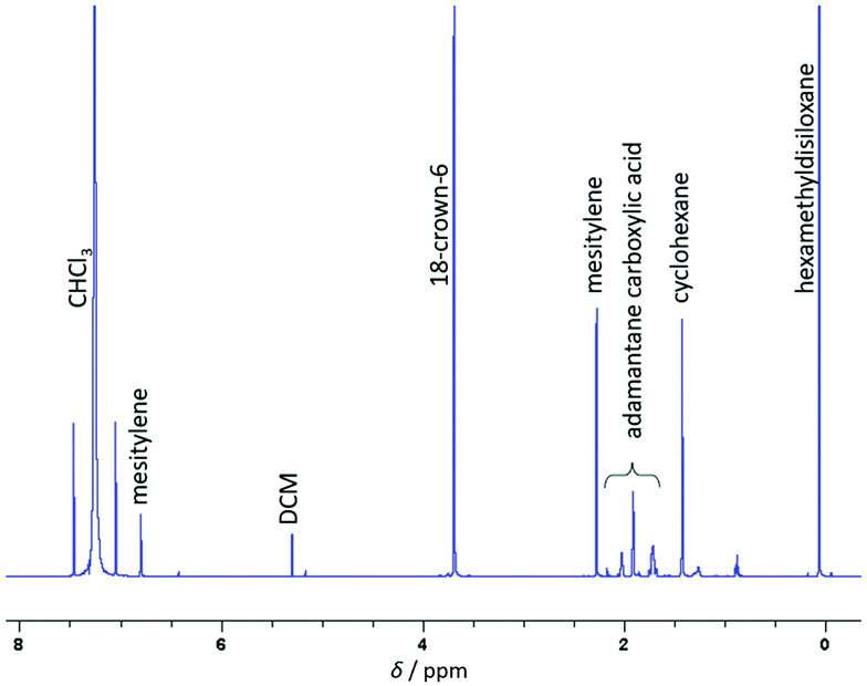Fig. 1 ¹H NMR spectrum of DOSY test solution. All species have simple, non-overlapping spectra with ≤ 3 signals in the ppm range used.

Despite having to deal with substantial linear displacement velocities of around 5 mm s⁻¹ at flow rates of 4 mL min⁻¹,§ convection compensation seemed promising in obtaining meaningful diffusion data from the flowing sample. Fig. 2 shows example data of the test mixture used for a diffusion delay (Δ) of 0.025 s and a gradient pulse length (δ/2) of 1000 μs (experiment C) at various flow rates. The observed diffusion coefficient D_flow increased with increasing flow rate for all molecules, as did the error associated with the measurement as derived from the fit of the 16-point DOSY curve. With acquisition parameters C the increase in D_flow was relatively small (up to 18%) and linear; with some of the larger Δ values, the increase was greater and no longer linear (see Fig. S1–S5, ESI†).

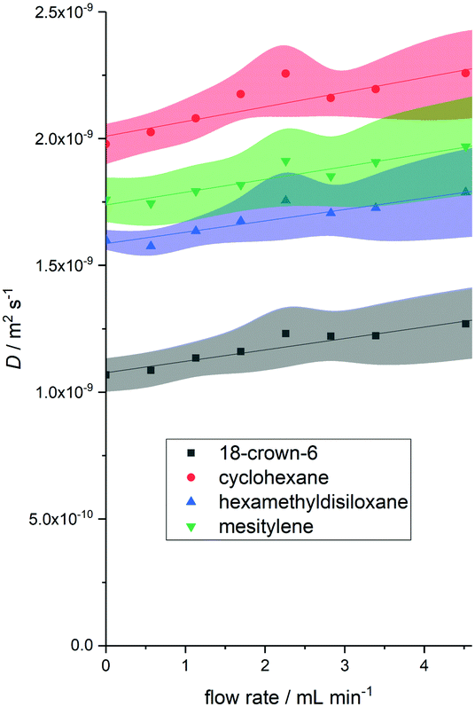Fig. 2 Example graph of observed diffusion coefficients against flow rate for four small molecules (Fig. 1, using acquisition parameters C from Table 1 (Δ = 0.025 s and δ/2 = 1000 μs). Shaded regions represent DOSY fit error margins.

It is worth noting that when flow rates were kept below 2 mL min⁻¹ and Δ was small, the absolute values obtained for D were within the error obtained from the curve fit of a static measurement (vide infra). This means that accurate diffusion coefficients may be obtained at low flow rates without the need for correction. Analysing the effects of higher flow velocities included correlating the average gradients of D_flow against flow rate for all molecules studied with acquisition parameter settings A–J to give an indication of the magnitude of the flow effect on measured D (i.e. the accuracy of the experiment) and the fit errors obtained at 4 mL min⁻¹ to show the measurement precision. The averages of these values across all five molecules plotted over Δ and δ/2 are shown in Fig. 3.

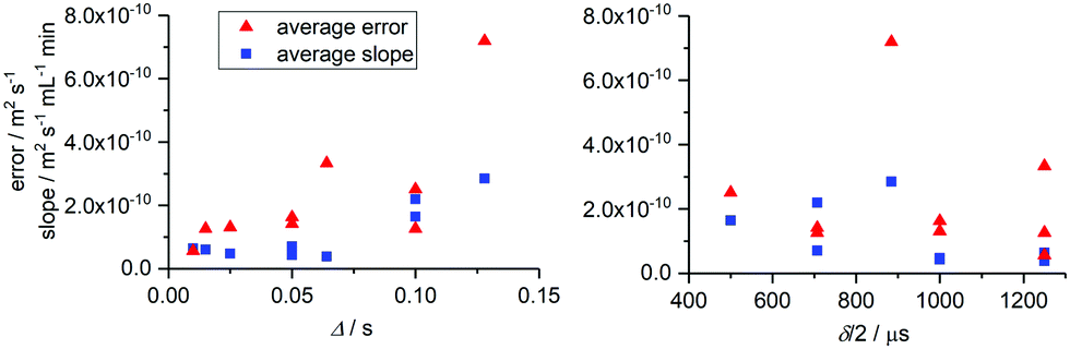Fig. 3 Average measurement errors at 4 mL min⁻¹ sample flow and gradients of D vs. flow rate across all molecules from Fig. 1 plotted as a function of Δ (left) and δ/2 (right). Errors associated with static measurements for all acquisition parameters used are shown in Fig. S6 (ESI†).

As can be seen from the average slope values in Fig. 3 (blue squares), the effect of flow was almost negligible for all experiments where Δ ≤ 0.064 s. For Δ ≥ 0.10 s, flow effects on the measured diffusion coefficients became more significant, giving rise to increasing levels of distortion and reducing precision (red triangles). The precision of the measurement can also be seen to decrease across the range of Δ values tested, and errors became noticeably larger once Δ exceeded 0.05 s. Therefore, smaller diffusion delays in the range of 0.025–0.050 s are recommended for convection compensated FlowDOSY measurements. Since delays of 0.05–0.1 s are typically used for static small molecule DOSY,²¹ a value of 0.05 s should be a good starting point in most cases. δ/2 had less effect than Δ on the observed diffusion coefficients and associated errors (Fig. 3 right hand side) and may thus be set to any desired value up to the safety threshold of the probe used.

Testing the limits of the effective acquisition parameter settings D (Table 1), we observed that as the flow rate exceeded 6 mL min⁻¹ the deviation of D_flow from the static value became much more pronounced and the measurement errors increased significantly (Fig. 4) which we ascribe to increasing contributions from turbulent flow.

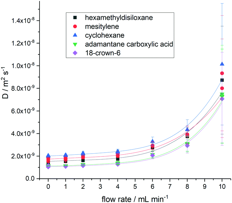Fig. 4 Plot of measured diffusion coefficients for five molecules (Fig. 1) at flow rates up to 10.0 mL min⁻¹ using acquisition parameters D from Table 1 (Δ = 0.05 s and δ/2 = 707 μs). Data are fit to fourth order polynomials to illustrate the trends.

For use in online reaction monitoring the linearity and precision of FlowDOSY data are more important than accuracy, as with a robust correlation it would be possible to back-calculate the intrinsic molecular diffusion values D_static from flow measurements in a manner similar to flow correction factors for peak integrals.¹ A plot of static versus flow diffusion values showed excellent linearity and virtually identical flow effects for all molecules in our test mixture up to ∼6 mL min⁻¹ (Fig. 5), suggesting a simple relationship of D_static = D_flow – χ_flow. Using convection compensated FlowDOSY with suitable acquisition parameters (such as C or D, Table 1) it is therefore possible to determine indirectly the intrinsic diffusion coefficient of an unknown molecule in a flowing mixture from a simple calibration using molecules whose D_static have been measured under comparable conditions (most importantly temperature and solvent viscosity). Note that any χ_flow correction will be specific to the size and geometry of the flow device used but does not depend on any correlation between diffusion coefficient and either molecular weight or hydrodynamic radius, and may thus be used for any molecule regardless of shape. Once intrinsic diffusion coefficients have been derived from the flow data, previously published methods can be applied for an estimation of molecular size and weight.^7,22

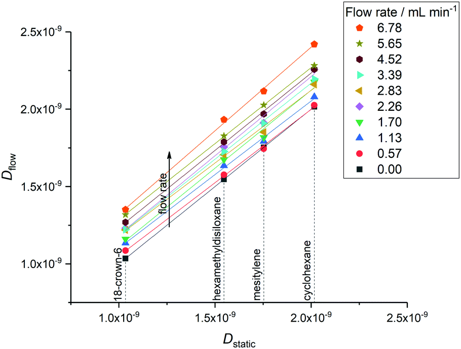Fig. 5 Correlation of flow diffusion coefficients with static diffusion coefficients for four small molecules (Fig. 1) at nine non-zero flow rates. Diffusion coefficients obtained using acquisition parameters C from Table 1 (Δ = 0.025 s and δ/2 = 1000 μs).

Although all experiments were carried out with a calibrated pump that delivered accurate average flow rates as set, the peristaltic model used is known to have a pulsation of ±14% at a frequency of 0.33 Hz.²³ With diffusion delay values of 10–150 ms these oscillations may be expected to impact FlowDOSY results obtained from averaging 16 scans, as there will be a periodic variation of sample flow velocities in the active volume during acquisition.

We thus reinvestigated the optimised, convection compensated FlowDOSY experiment using a low pulsation rotary piston pump that smoothly delivers the sample flow at <1% variation²³ (for details see the ESI†). A side-by-side comparison of the same experiment using the peristaltic pump showed that there was almost no flow effect on the DOSY data up to 4 mL min⁻¹ when using the low pulsation pump (Fig. 6).

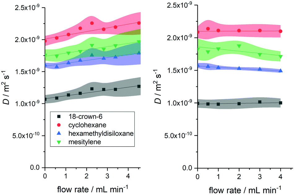Fig. 6 Difference in flow effects on measured diffusion coefficient of four small molecules (Fig. 1) using peristaltic (left) and rotary piston pumps (right). Diffusion coefficients obtained using acquisition parameters C from Table 1 (Δ = 0.025 s and δ/2 = 1000 μs).

Remarkably, any variations in the measured diffusion coefficients D_flow were within the error of the experiment, and absolute errors were the same or smaller in flow than under static conditions (see also the Fig. S12 and S13, ESI†). These results show flow effects in DOSY measurements of continuously moving samples to be mostly a reflection of non-ideal flow such as turbulences and eddies, and that convection compensation with suitable acquisition parameters can effectively deal with constant (non-pulsed) linear sample displacement along the gradient axis used to directly yield accurate and precise molecular diffusion values at flow rates of at least up to 4 mL min⁻¹.

For reaction monitoring experiments aimed at following molecular transformations over time, short measurement times will be advantageous as they allow for collecting more information over the course of a reaction. ¹H DOSY experiments typically employ acquisition times of around 1.3 s and recycle delays of 2 s, resulting in experiment times of 10–20 min for a high quality DOSY spectrum with 16 scans. We found that the acquisition times and recycle delays could be reduced to 1.0 s and 1 μs respectively¶ without compromising either the S : N or the accuracy of the diffusion coefficient as long as sufficient dummy scans were included (8 in this case). This reduced the experiment time for a high resolution DOSY experiment (16 gradients strengths, 16 scans at each gradient strength) either statically or in flow to less than 5 min (for details see Tables S3–S5, ESI†).

In addition to a simple adjustment that allows increasing temporal resolution three to four-fold without compromising data quality, we have shown three ways of obtaining accurate diffusion coefficients on a flowing sample using a convection compensated DOSY pulse sequence with a standard single gradient NMR probe. In order of increasing effectiveness, they are: (i) using a low flow rate in the region of 1–2 mL min⁻¹ and a short diffusion delay time of Δ < 0.05 s; (ii) making a calibration curve to correct for linear flow effects at flow rates up to 6 mL min⁻¹; and (iii) using a high precision pump with minimal pulsation which effectively eliminates flow effects. More detailed recommendations can be found in the supporting information (Table S7, ESI†). The development of FlowDOSY offers a new tool for online reaction monitoring that we expect to prove useful in investigating and understanding many new and old reaction systems. Quickly measuring accurate diffusion data on flowing mixtures in a non-invasive way gives access to valuable information on molecular size, aggregation and mobility that complements existing reaction monitoring techniques such as online GPC. WET solvent suppression, which we have previously found to work well in flow,¹ may be incorporated for applications in non-deuterated solvents where dynamic range issues may be encountered. The principles shown likely extend to heteronuclear DOSY experiments and also apply to low field (benchtop) NMR instruments with gradients to open up a wide range of applications in many different areas.

This work was supported by the Royal Society (Fellowship UF160458 to UH), the EPSRC (Dynamic Reaction Monitoring Facility EP/P001475/1 and Centre for Doctoral Training in Sustainable Chemical Technologies EP/L016354/1) and the University of Bath. We thank Peter Gierth (Bruker UK) for support and assistance with this project.

Conflicts of interest

There are no conflicts to declare.

Notes and references

1. A. M. R. Hall, J. C. Chouler, A. Codina, P. T. Gierth, J. P. Lowe and U. Hintermair, Catal. Sci. Technol., 2016, 6, 8406–8417.
2. D. B. G. Berry, A. Codina, I. Clegg, C. L. Lyall, J. P. Lowe and U. Hintermair, Faraday Discuss., 2019, 220, 45–57.
3. D. Lynch, R. M. O’Mahony, D. G. McCarthy, L. M. Bateman, S. G. Collins and A. R. Maguire, Eur. J. Org. Chem., 2019, 3575–3580.
4. A. M. R. Hall, R. Broomfield-Tagg, M. Camilleri, D. R. Carbery, A. Codina, D. T. E. Whittaker, S. Coombes, J. P. Lowe and U. Hintermair, Chem. Commun., 2017, 54, 30–33.
5. A. Bara-Estaún, C. L. Lyall, J. P. Lowe, P. G. Pringle, P. C. J. Kamer, R. Franke and U. Hintermair, Faraday Discuss., 2021, 229, 422–442.
6. A. M. R. Hall, P. Dong, A. Codina, J. P. Lowe and U. Hintermair, ACS Catal., 2019, 9, 2079–2090.
7. R. Evans, G. Dal Poggetto, M. Nilsson and G. A. Morris, Anal. Chem., 2018, 90, 3987–3994.
8. S. Augé, P.-O. Schmit, C. A. Crutchfield, M. T. Islam, D. J. Harris, E. Durand, M. Clemancey, A.-A. Quoineaud, J.-M. Lancelin, Y. Prigent, F. Taulelle and M.-A. Delsuc, J. Phys. Chem. B, 2009, 113, 1914–1918.
9. N. Cherifi, A. Khoukh, A. Benaboura and L. Billon, Polym. Chem., 2016, 7, 5249–5257.
10. W. Li, H. Chung, C. Daeffler, J. A. Johnson and R. H. Grubbs, Macromolecules, 2012, 45, 9595–9603.
11. P.-J. Voorter, A. McKay, J. Dai, O. Paravagna, N. R. Cameron and T. Junkers, Angew. Chem., Int. Ed., 2022, 61(5), e202114536.
12. S. Sato, D. Gondo, T. Wada, S. Kanehashi and K. Nagai, J. Appl. Polym. Sci., 2013, 129, 1607–1617.
13. H. J. Reich, Chem. Rev., 2013, 113, 7130–7178.
14. W. Hiller, Macromol. Chem. Phys., 2019, 220, 1900255.
15. D. Li, R. Hopson, W. Li, J. Liu and P. G. Williard, Org. Lett., 2008, 10, 909–911.
16. D. Li, I. Keresztes, R. Hopson and P. G. Williard, Acc. Chem. Res., 2009, 42, 270–280.
17. P. A. Keifer, Annu. Rep. NMR Spectrosc., 2007, 62, 1–47.
18. J. H. Vrijsen, I. A. Thomlinson, M. E. Levere, C. L. Lyall, M. G. Davidson, U. Hintermair and T. Junkers, Polym. Chem., 2020, 11, 3546–3550.
19. A. Jerschow and N. Müller, J. Magn. Reson., 1997, 125, 372–375.
20. P. Groves, Polym. Chem., 2017, 8, 6700–6708.
21. T. D. W. Claridge, High-Resolution NMR Techniques in Organic Chemistry, Elsevier, 2016.
22. C. Su, R. Hopson and P. G. Williard, J. Am. Chem. Soc., 2013, 135, 14367–14379.
23. A. Saib, A. Bara-Estaún, O. J. Harper, D. B. G. Berry, I. A. Thomlinson, R. Broomfield-Tagg, J. P. Lowe, C. L. Lyall and U. Hintermair, React. Chem. Eng., 2021, 6, 1548–1573.

---

Footnotes

† Electronic supplementary information (ESI) available: Materials & methods, experimental details, additional data and plots including the effects of temperature regulation and injection capillary. See DOI: https://doi.org/10.1039/d2cc03054c

‡ During peer review of this manuscript a paper reporting fast and accurate FlowDOSY methods was published by J–N. Dumez and co-workers [DOI: 10.1002/chem.202201175]. Their approach, developed independently to our work, uses orthogonal gradients to eliminate the effect of flow pulsation and includes a single-scan DSTE DOSY pulse sequence, methods that are complementary to those reported in this paper.

§ At 4 mL min⁻¹ the average residence time of the sample in the detector region is around 7 seconds.

¶ A minimum repetition time of 1 s is quoted as safety threshold for our probe by the manufacturer.

---