
 Open Access Article
 This Open Access Article is licensed under a
 Creative Commons Attribution 3.0 Unported Licence
Towards fully optimised and automated ESR spectroscopy†‡
Jean-Baptiste
Verstraete
a,
Jonathan R. J.
Yong
a,
David L.
Goodwin
 a,
William K.
Myers
b and
Mohammadali
Foroozandeh
*a
a,
William K.
Myers
b and
Mohammadali
Foroozandeh
*a
aChemistry Research Laboratory, University of Oxford, Mansfield Road, Oxford OX1 3TA, UK. E-mail: mohammadali.foroozandeh@chem.ox.ac.uk
bCentre for Advanced ESR, Inorganic Chemistry Laboratory, University of Oxford, South Parks Road, Oxford OX1 3QR, UK
First published on 30th August 2022
Abstract
To address the problems of instrumental imperfection and time-consuming experimental setup in electron spin resonance (ESR), we present ESR-POISE, a user-friendly software package for fully automated and fast on-the-fly optimisation and acquisition of ESR experiments. This open-source package interfaces with Bruker's Xepr software and allows scientists to run user-defined optimisations.
Electron spin resonance (ESR), also known as electron paramagnetic resonance (EPR), is one of the most important analytical techniques available to scientists in chemistry, biology, physics, and materials science, but unfortunately, hardware performance is not able to keep up with the rapid growth in its applications.1–3 Most ESR experiments require an experienced operator to tweak experimental parameters to improve the result of the experiment. However, this costs valuable time and effort, and a lack of experience, or constraints on experimental time, can easily render this often long, laborious, and complicated tweaking procedure impractical, especially in the case of complex multiple-parameter experiments.
A viable solution to these challenges is the automated feedback control of the experiment, which can be carried out independent of the operator's expertise or the sample under study. Such an optimisation algorithm would evaluate a suitable cost function which reflects the quality of experimental results, and change the requisite experimental parameters appropriately at each measurement. After a number of measurements, the algorithm converges to the best set of experimental parameters, delivering the most desirable result (Fig. 1). Although such optimisation techniques have been used in areas such as laser spectroscopy,4–6 quantum information processing,7 and organic synthesis,8–10 they are noticeably underused in magnetic resonance, with very few relevant publications in nuclear quadrupole resonance (NQR),11 nuclear magnetic resonance (NMR),12 and ESR itself.13
 | ||
| Fig. 1 (a) Flowchart for an ESR-POISE optimisation. (b) 2D map showing the magnitude of the cost function for the flip angle optimisation as a function of pulse length and amplitude, obtained by a conventional grid search covering the entire parameter space (198 measurements in total). Brighter colours indicate a lower value of the cost function, i.e. better performance. The train of orange arrows shows the stepwise trajectory of the cost function for the POISE optimisation (12 measurements). Two last iterations were omitted for visual clarity. The black dot indicates the minimum found by the optimiser, and the black cross the minimum found with the full grid-search. | ||
Here, we present, for the first time, a general-purpose, fully-automated routine that is capable of on-the-fly optimisation and automation of many ESR experimental procedures. This user-friendly Python package, ESR-POISE (Parameter Optimisation by Iterative Spectral Evaluation), is fully compatible with commercial ESR spectrometers via an interface with Bruker's Xepr software and allows users to define personalised procedures. The proposed method, taking advantage of derivative-free optimisation algorithms,14–16 provides substantial speed-up in experiment setup and opens the path towards fully automated and optimised ESR spectroscopy.
ESR-POISE provides multiple optimisation algorithms,14–16,18 but all the results presented in the main text of this article were produced using BOBYQA (Bound Optimization BY Quadratic Approximation), a trust-region interpolation method,15,16 as it showed superior speed and stability.12 For more information on other algorithms, please refer to the ESI.†
One attractive application of on-the-fly optimisation is the automation of procedures that are performed routinely on almost every sample. In ESR, the adjustment of the signal phase to acquire an in-phase echo is one such procedure. By maximising the real part of the echo intensity (Fig. 2a) ESR-POISE finds the correct signal phase with 10 measurements in approximately 30 seconds (Table S2, ESI†). This optimisation can optionally be combined with a second one to minimise the imaginary part of the echo, which requires 30 more seconds for 10 additional measurements (Table S3, ESI†). This composite procedure would closely resemble what an experienced user would perform on the spectrometer. Although single-parameter optimisations such as these can be performed fairly easily by skilled users, the automation of the entire procedure is still highly desirable. Additional examples of single-parameter optimisations are presented in Tables S8–S10 (ESI†).
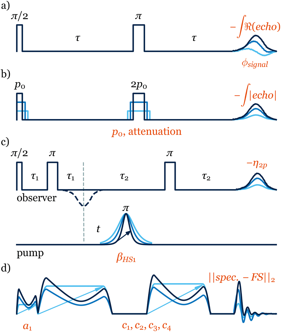 | ||
| Fig. 2 Schematic representations of pulse sequences and elements subjected to optimisations: (a) phase of the detected signal after a Hahn echo, (b) flip angles of 90° and 180° pulses of a Hahn echo, parametrized by pulse length and amplitude, (c) The HS pump pulse in a 4-pulse DEER experiment, and (d) pulse waveforms in the CHORUS sequence. Parameters subjected to the optimisation and their corresponding cost function are indicated in orange, respectively, below and above each sequence. | ||
ESR-POISE can also tackle more challenging multi-parameter experiments, for example, the standard flip angle calibration for 90° excitation and 180° refocusing pulses in a Hahn echo19 pulse sequence, to improve the magnitude of the detected signal. The flip angle of a pulse is adjusted using the pulse duration and its power amplitude. As most ESR spectrometers have a limited precision for defining the pulse duration, while maximising the echo, we targeted the shortest possible pulse duration that delivers a desired flip angle (see Fig. 2). ESR-POISE converged to a highly accurate optimum with only 12 function evaluations, 16 times less than the conventional grid-based parameter search, requiring 198 function evaluations (Fig. 1b and Table S4, ESI†).
ESR-POISE is a versatile tool that goes beyond standard parameters such as the ones mentioned above. It can also handle user-defined parameters and cost functions and provides users with easy access to parameters which cannot be readily modified at the spectrometer. An example of a procedure using custom parameters and cost functions is the optimisation of the pump pulse in a four-pulse double electron-electron resonance (DEER), one of the most commonly used ESR experiments (Fig. 2c).20 The DEER experiment uses two pulse channels: one pump channel with an inversion pulse which is shifted in time (t in Fig. 2c) to reveal the evolution of the dipolar coupling, and a second observer channel for detection of the resulting echo. The dipolar coupling between two electrons can be obtained from the spin-echo modulation in the DEER trace, and is often used for distance measurements. To obtain the best DEER traces, the pump and observer pulses should cover as much of the EPR spectrum as possible while not overlapping.
Application of a shaped band-selective inversion pump pulse21,22 seems to offer a solution. However, the choice of appropriate shape parameters is not trivial and has been the subject of extensive investigations.23,24 Here, the goal is to adjust the selectivity of a hyperbolic secant (HS) pulse by finding a suitable truncation factor β (see eqn (S1) and (S2), ESI†). Although numerical simulations can be used to study the effects of the pulse, they cannot easily take into account important hardware effects on the shaped pulse and, in this case, did not suggest a suitable value for β (see Fig. S1, ESI†). In contrast, ESR-POISE circumvents this problem and proved to be efficient in finding an appropriate shape. The parameter η2p,21,25,26 the intensity difference between the first maximum and the first dip in the DEER trace, was used for the cost function, which allows determination of the DEER trace quality without having to record it fully. A three-minute optimisation led to ∼20% increase in η2p (see Table S5, ESI†). The full trace was then recorded (in ∼3 hours), showing that the gain was retained with a 23% increase in the modulation depth (Fig. 3b).
 | ||
| Fig. 3 Cartesian representation of the HS pump pulse in a 4-pulse DEER experiment, (a) before (β = 10), and (b) after (β = 6) optimisation, with (c) corresponding full DEER traces for bisnitroxide (Scheme 1). | ||
Thanks to the capabilities of the POISE method, one can explore even larger parameter spaces that are more challenging and, in many cases, impossible to cover by brute force methods. One example is the amplitude optimisation of the excitation sequence, CHORUS (CHirped, ORdered pulses for Ultra-broadband Spectroscopy),27 (Fig. 2d). Due to the spectrometer's non-linear response, each of the three chirped pulses needs to be calibrated individually to achieve a combination that maximises the tolerance of the sequence to hardware errors. Previously,27 this was achieved manually, where the amplitude of the 90° pulse was set up first, followed by a 2D grid search for amplitudes of two 180° pulses, using 50 steps for each pulse amplitude. This process, only using the on-resonance signal and neglecting the performance across the entire spectral width, required 2600 measurements to complete. In contrast, ESR-POISE can simultaneously optimise all three pulse amplitudes, with only 30 function evaluations (measurements), offering at least a 10-fold decrease in optimisation time (Table S6, ESI†).
An even more challenging case on an ESR spectrometer is when hardware design limitations, in particular resonators, distort shaped pulses produced by an arbitrary waveform generator (AWG). One can use a transfer function, a model that describes the effect of the hardware on a pulse, to create a compensated pulse. Different approaches have been proposed to find transfer functions in ESR.22,28,29 However, the transfer function is not only dependent on the hardware, but can also vary with the sample under investigation, making this procedure non-repeatable.
Here we show that, using an on-the-fly POISE optimisation, one can address both sample and instrument dependencies of the resonator effect in a far more efficient way. Although the approach presented here is general and can be applied to any shaped pulse or a sequence of shaped pulses, to represent a complex multi-pulse experiment with a disproportional non-linear response, we use the CHORUS sequence again. We aimed to achieve a fully compensated sequence that provides a uniform excitation across a large spectral window of interest. The norm of the difference between a normalised field-sweep spectrum (reference) and the CHORUS spectrum is used as the cost function.
Following an initial amplitude optimisation as described previously, we simultaneously optimised five parameters using ESR-POISE: four parameters for the transfer function (eqn (S6), ESI†) and the amplitude of the excitation pulse. The optimisation on a sample of bisnitroxide (Scheme 1) converged after 113 function evaluations, delivering a threefold decrease in the cost function (see Fig. 4c, d, and Table S7, ESI†). The optimisation took 23 minutes to produce compensated shapes (Fig. 4b). See Fig. S3–S6 and Table S7 (ESI†) for additional information. A corresponding full grid-based parameter search would have required about 530 million measurements and 200 years to run. Please note that similar results to Fig. 4d may be obtained using other methods proposed in the literature,22,28,29 albeit at the cost of some time-consuming manual calibration steps. ESR-POISE can be used to automate such routines should the user intend to employ a different procedure or objective function. Additionally, the application of ESR-POISE is not limited to modern ESR instruments, equipped with AWGs, and can be applied to any instrument where parametric optimisation of ESR experiments is required. One example of such optimisation is presented in Section 8 of the ESI.†
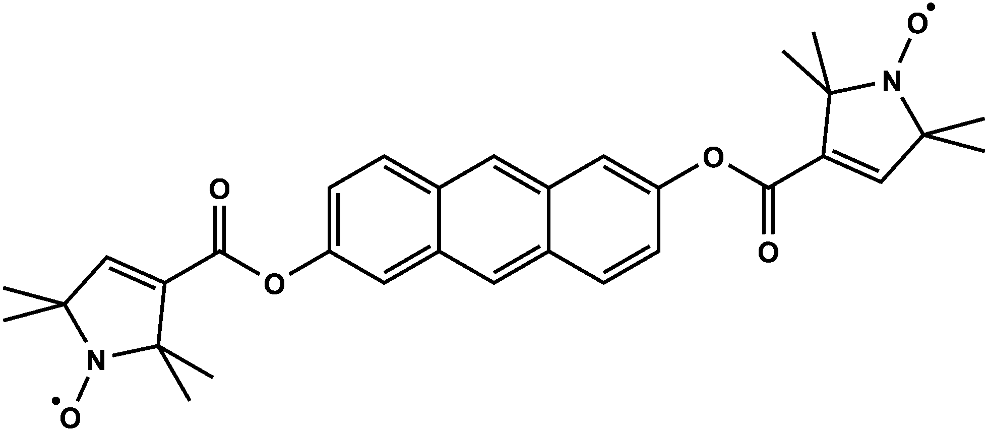 | ||
| Scheme 1 Bisnitroxide (2,6-bis[(((2,2,5,5-tetramethyl-1-oxypyrrolin3-yl)-carboxyl)oxy)]-anthracene),17 the sample used to produce the results of this study. | ||
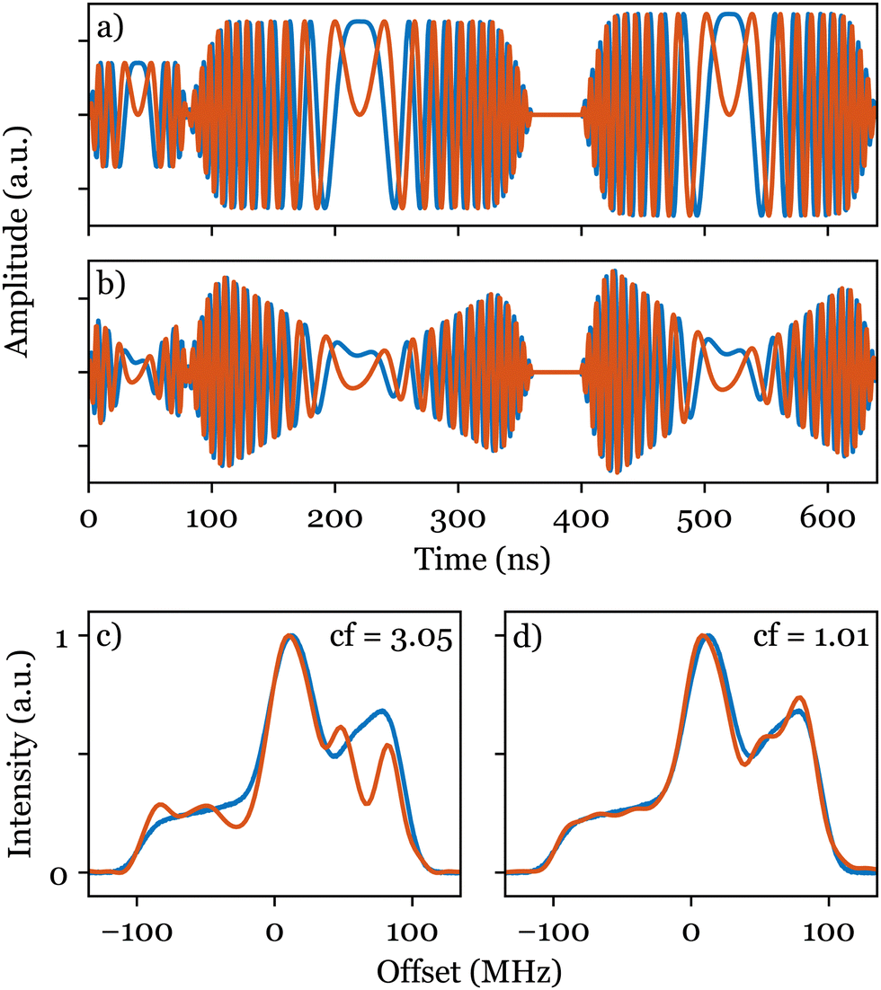 | ||
| Fig. 4 Cartesian representations of the CHORUS sequence: (a) without and (b) with compensation. Normalised experimental excitation spectra of bisnitroxide (Scheme 1) obtained with the CHORUS sequence (red) are shown in (c) before and (d) after amplitude optimisation and hardware compensation and are compared with the reference field-sweep spectrum (blue). The corresponding values of the cost function (cf) are shown in both cases. | ||
In conclusion, we have demonstrated that a diverse range of ESR experiments can be optimised in a fast and fully automated fashion. Notably, these include scenarios where multiple parameters are in play, and/or when these parameters are not immediately exposed to the user. The on-the-fly optimisations presented here can be further improved by developing more sophisticated models capturing the behaviour of the instrument's components, or by starting from a better initial guess. As an open-source platform for optimisation, ESR-POISE may be readily expanded with other optimisation algorithms via community participation. We believe that ESR-POISE can become a routinely used software by individual users, including chemists, physicists, biologists, materials scientists, and even professional ESR spectroscopists, where the capabilities of POISE for automation and optimisation can provide considerable savings in precious instrument time.
ESR-POISE can be most easily installed via the Python package manager pip; the source code is available on GitHub (https://github.com/foroozandehgroup/esrpoise) and its documentation at https://foroozandehgroup.github.io/esrpoise.
All experiments were run at X-band on an Elexsys E680 Bruker spectrometer, at a carrier frequency of 9.56 GHz (except for CHORUS compensation at 9.46 GHz and 9.56 GHz in ESI†). The temperature was set to 293 K for the signal phase optimisation, and to 70 K for all other optimisations.
This research was supported by the Royal Society (URF\R1\180233 and RGF\EA\181018), the John Fell OUP Research Fund (0007019), the EPSRC Doctoral Training Partnership, the University of Oxford Clarendon Fund, the EPSRC Centre for Doctoral Training in Synthesis for Biology and Medicine (EP/L015838/1) and associated industrial partners, the Centre for Advanced ESR (UK EPSRC EP/V036408/1 and EP/L011972/1), and the Department of Chemistry, University of Oxford. We thank Claudia Tait for useful discussions and feedback on the ESR-POISE package.
Conflicts of interest
There are no conflicts to declare.Notes and references
- A. Schweiger and G. Jeschke, Principles of pulse electron paramagnetic resonance, Oxford University Press, Oxford, 2001 Search PubMed.
- P. E. Spindler, P. Schops, W. Kallies, S. J. Glaser and T. F. Prisner, J. Magn. Reson., 2017, 280, 30–45 CrossRef CAS PubMed.
- G. Jeschke, J. Magn. Reson., 2019, 306, 36–41 CrossRef CAS.
- C. J. Bardeen, V. V. Yakovlev, K. R. Wilson, S. D. Carpenter, P. M. Weber and W. S. Warren, Chem. Phys. Lett., 1997, 280, 151–158 CrossRef CAS.
- N. H. Damrauer and G. Gerber, Quantum Control by Adaptive Femtosecond Pulse Shaping, American Chemical Society, 2002, vol. 821, book section 13, pp. 190–206 Search PubMed.
- A. Weigel, A. Sebesta and P. Kukura, J. Phys. Chem. Lett., 2015, 6, 4032–4037 CrossRef CAS PubMed.
- D. J. Egger and F. K. Wilhelm, Phys. Rev. Lett., 2014, 112, 240503 CrossRef CAS PubMed.
- R. A. Skilton, A. J. Parrott, M. W. George, M. Poliakoff and R. A. Bourne, Appl. Spectrosc., 2013, 67, 1127–1131 CrossRef CAS PubMed.
- D. E. Fitzpatrick, C. Battilocchio and S. V. Ley, Org. Process Res. Dev., 2016, 20, 386–394 CrossRef CAS.
- V. Fath, N. Kockmann, J. Otto and T. Röder, React. Chem. Eng., 2020, 5, 1281–1299 RSC.
- C. Monea, J. Magn. Reson., 2020, 321, 106858 CrossRef CAS PubMed.
- J. R. J. Yong and M. Foroozandeh, Anal. Chem., 2021, 93, 10735–10739 CrossRef CAS PubMed.
- D. L. Goodwin, W. K. Myers, C. R. Timmel and I. Kuprov, J. Magn. Reson., 2018, 297, 9–16 CrossRef CAS PubMed.
- J. A. Nelder and R. Mead, Comput. J., 1965, 7, 308–313 CrossRef.
- M. J. D. Powell, University of Cambridge, 2009, DAMTP 2009/NA06.
- C. Cartis, J. Fiala, B. Marteau and L. Roberts, ACM Trans. Math. Softw., 2019, 45, 32 CrossRef.
- R. G. Larsen and D. J. Singel, J. Chem. Phys., 1993, 98, 5134–5146 CrossRef CAS.
- J. J. E. Dennis and V. Torczon, SIAM J. Control, 1991, 1, 448–474 Search PubMed.
- E. L. Hahn, Phys. Rev., 1950, 80, 580–594 CrossRef.
- M. Pannier, S. Veit, A. Godt, G. Jeschke and H. W. Spiess, J. Magn. Reson., 2000, 142, 331–340 CrossRef CAS.
- P. E. Spindler, S. J. Glaser, T. E. Skinner and T. F. Prisner, Angew. Chem., Int. Ed., 2013, 52, 3425–3429 CrossRef CAS PubMed.
- A. Doll, S. Pribitzer, R. Tschaggelar and G. Jeschke, J. Magn. Reson., 2013, 230, 27–39 CrossRef CAS.
- M. Teucher and E. Bordignon, J. Magn. Reson., 2018, 296, 103–111 CrossRef CAS PubMed.
- A. Scherer, S. Tischlik, S. Weickert, V. Wittmann and M. Drescher, Magn. Reson., 2020, 1, 59–74 CrossRef.
- A. Doll, M. Qi, N. Wili, S. Pribitzer, A. Godt and G. Jeschke, J. Magn. Reson., 2015, 259, 153–162 CrossRef CAS.
- C. E. Tait and S. Stoll, Phys. Chem. Chem. Phys., 2016, 18, 18470–18485 RSC.
- J.-B. Verstraete, W. K. Myers and M. Foroozandeh, J. Chem. Phys., 2021, 154, 094201 CrossRef CAS.
- P. E. Spindler, Y. Zhang, B. Endeward, N. Gershernzon, T. E. Skinner, S. J. Glaser and T. F. Prisner, J. Magn. Reson., 2012, 218, 49–58 CrossRef CAS PubMed.
- T. Kaufmann, T. J. Keller, J. M. Franck, R. P. Barnes, S. J. Glaser, J. M. Martinis and S. Han, J. Magn. Reson., 2013, 235, 95–108 CrossRef CAS PubMed.
Footnotes |
| † Electronic supplementary information (ESI) available: Details of experiments, complementary simulations, and additional remarks on the optimisation process. See DOI: https://doi.org/10.1039/d2cc02742a |
| ‡ Waveforms for the CHORUS sequence, simulations of resonator compensation, and experimental data are also publicly hosted on Mendeley and available via DOI: https://doi.org/10.17632/mg2yx7tzdn.2. |
| This journal is © The Royal Society of Chemistry 2022 |