SHARPER-enhanced benchtop NMR: improving SNR by removing couplings and approaching natural linewidths

Abstract

We present a signal enhancement strategy for benchtop NMR that produces SNR increases on the order of 10 to 30 fold by collapsing the target resonance into an extremely narrow singlet. Importantly, the resultant signal is amenable to quantitative interpretation and therefore can be applied to analytical applications such as reaction monitoring.

---

NMR spectroscopy is a well-established technique for reaction monitoring on high field NMR spectrometers, and more recently also on benchtop instruments.^1–3 In principle, the reaction rate can be determined by monitoring the integral intensity of a single signal of a reactant. In this context, any splitting of the observed signal by scalar couplings decreases the signal-to-noise ratio (SNR) and therefore the removal of such splitting is desirable. The SHARPER (Sensitive, Homogeneous And Resolved PEaks in Real time) experiment⁴ achieves this by the means of data acquisition interrupted by 180° refocussing pulses.^5–8 When non-selective pulses are used, all heteronuclear couplings are removed, while in selSHARPER, where selective 180° pulses are used, the homonuclear couplings also vanish; in both instances no X-channel pulses are required. As the SHARPER signal acquisition is embedded within a CPMG pulse sequence,^9,10 it also eliminates the effects of magnetic field inhomogeneity, generating extremely narrow singlets with linewidths of a fraction of 1 Hz.

The SHARPER technique has been applied to a range of nuclei (¹H, ¹⁹F and ³¹P) and tested on monitoring a variety of chemical reactions under challenging conditions, such as gas sparging. Significant SNR gains (up to 20 fold for reasonably well shimmed samples, much higher when the B₀ homogeneity is poor) by SHARPER experiments substantially reduce the required sample quantities and/or experimental times, making reaction monitoring more efficient and allowing monitoring of faster reactions.⁴

Fluorinated organic molecules account for 20 and 60%, respectively, of pharmaceuticals¹¹ and agrochemicals¹² produced today. To support their production, development of efficient and environmentally safe fluorination methods¹³ positioned fluorine chemistry among the most active fields of organic chemistry, with efficient reaction monitoring making important contributions.¹⁴ Fortuitously, due to its large chemical shift dispersion, ¹⁹F NMR can take full advantage of SHARPER sequences, where even at low magnetic fields, the ¹⁹F resonances often are sufficiently isolated to allow for their selectively manipulation required by selSHARPER sequences.

Due to the close Larmor frequencies of ¹⁹F and ¹H at 1-2T, the same coil can be used for both nuclei, hence most benchtop systems are typically capable of operating at both frequencies. Nevertheless, there are challenges for ¹⁹F NMR at benchtop spectrometers. The probes are usually tuned to favour the sensitivity of ¹H detection at the expense of ¹⁹F. The SNRs of ¹⁹F spectra is further compromised by splittings caused by numerous J_HF and J_FF couplings, complex peak shapes and lower field homogeneity compared to high-field spectrometers. In addition, efficient ¹H decoupling to remove the J_HF couplings is very challenging when the same coil is used for ¹H and ¹⁹F.

SHARPER presents a potential solution to all these problems, however, the existing versions require pulsed field gradients (PFGs) for both spin selection (in selSHARPER) and during the acquisition but PFGs are not standard on many benchtop NMR spectrometers¹⁵ and shaped selective pulses are currently only supported on certain models. Because of these hardware limitations, SHARPER sequences have yet to be implemented on benchtop instruments.

In this Communication we present several variations of the SHARPER technique that address these issues, including removal of PFGs from the acquisition loops and/or from the initial resonance selection step. We also introduce protocols for processing of spectra that further improve SNRs and generate high quality quantitative data required for reaction monitoring. Nevertheless, it should be noted that the developed acquisition and processing protocols are equally valuable for experiments performed on high-field instruments.

The first modification of the original SHARPER sequences involves removing PFGs from the acquisition loops, which was made possible by adjusting the phase cycle of the train of the 180° pulses (Fig. 1a). This allows for more time to be spent on signal acquisition, reducing undesirable relaxation and diffusion effects and producing narrower and more intense signals. Higher SNRs compared to the original experiments are obtained, improving the precision of integrals. A comparison of the two approaches is presented in the ESI,† Fig. S1. This modification is applied to all pulse sequences introduced here.

Fig. 1 SHARPER pulse sequences implemented on benchtop NMR spectrometers. The filled and empty rectangles represent 90° and 180° hard pulses, while smoothed empty and shaded shapes depict selective 180° and 270° pulses, respectively. τ = AQ/(2n), where AQ is the total acquisition time and n is the number of loops. (a) SHARPER and (d) 270 G-selSHARPER: φ₁ = x; φ₂ = y, −y; ψ = x. (b) SPFGSE-selSHARPER and (c) SE-selSHARPER, φ₁ = x; φ₂ = x, y; φ₃ = 2y, 2(−y); ψ = x, −x; the minimum number of scans is 1 for (a)–(c) and 2 for (d). Pulse programs for Spinsolve NMR spectrometers will be provided upon request.

A complete removal of PFGs is possible by replacing the initial single pulsed field gradient spin echo (SPFGSE, Fig. 1b) by other means of signal selection. Two alternative selSHARPER sequences were tested. The first, SE selSHARPER (Fig. 1c), uses two scans to cancel off-resonance signals without requiring PFGs, while the second, 270 G selSHARPER (Fig. 1d), uses a 270° Gaussian pulse.¹⁶ The latter is more suited for faster chemical reactions, where acquisition of a single scan per time point is required. It should be noted that some benchtop systems have non-linear amplifiers and calibration of power levels using standard procedures and concentrated samples is required; this can be fine-tuned efficiently by the selSHARPER pulse sequence on real, diluted samples as detailed in the ESI.†

A less general, but effective application of the pulse sequence in Fig. 1a achieves signal selection when only two resonances are present in the spectrum. This could be the case when a reaction of a mono-fluorinated compound is monitored, with the reactant and the product producing one ¹⁹F signal each. Referred to here as rectangular selSHARPER, this pulse sequence uses lower power rectangular pulses adjusted in duration so that the first zero point of their excitation (inversion) profile falls at the frequency of the off-resonance signal. The length of such 90° and 180° pulses is calculated from the frequency difference between the two signals, Δ in Hz, as and , respectively.¹⁷ Alternatively, the pw₁₈₀ is set to 2pw₉₀ calculated by the first equation and the power level is kept constant for both pulses. This positions the second zero point of the sinc lobes of the 180° rectangular pulse at the frequency of the off-resonance signal.

The implementation of SHARPER experiments for benchtop NMR spectrometers is illustrated using fluorobenzene, 1, pentafluorobenzene, 2, and 2,2,3,3,3-pentafluoropropanol, 3, as model compounds. Their ¹H and ¹⁹F spectra are presented in Fig. S2 (ESI†). Parameters of SHARPER experiments can also be found in the ESI.† Fluorobenzene, 1, which contains a single ¹⁹F atom and thus is suitable for testing both the non-selective and selective SHARPER pulse sequences was used initially. The spectra (Fig. 2) were acquired on a 60 MHz Spinsolve Ultra spectrometer without a dedicated gradient channel and the PFGs required for the SPFGSE selSHARPER experiments were generated by a shim coil. With the exception of the SE selSHARPER pulse sequence (Fig. 1c), which requires two scans, all other spectra can be acquired using a single scan. Additional phase cycling of the 180° pulses (Fig. 1a, φ₂ = y, −y) applicable to all sequences improves the quality of the spectra (Fig. S3, ESI†).

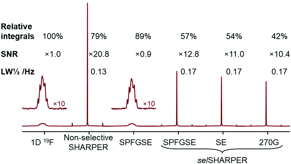Fig. 2 Comparing relative integrals, SNRs and signal linewidths (relative to the 1D ¹⁹F spectrum of 1) for SPFGSE, non-selective SHARPER and three selSHARPER spectra acquired at 56.46 MHz using 4 scans and fully relaxed spins. Spectra are plotted on the same scales. Only real parts of FIDs were Fourier transformed (see discussion in the text for the choice of acquisition and processing parameters).

All spectra were acquired using 4 scans by keeping identical repetition time ∼5T₁ of ¹⁹F in 1 and processed following the guidelines presented later in the paper. Significant SNR improvements relative to the standard 1D ¹⁹F spectrum were achieved: 20.8× for the non-selective SHARPER and up to 12.8× for the selective pulse sequences, despite some losses in observed integral intensities, particularly when selective pulses were used in the acquisition loops. These losses are attributed to the B₁ inhomogeneity affecting selective pulses. Even larger improvements per unit of time in SNR are obtained for 1-scan spectra as illustrated in the ESI.† The use of 5 ms selective 180° pulses in selSHARPER caused a ∼20% increase in signal line widths (Δ_1/2 = 0.18 Hz), compared to the non-selective SHARPER (Δ_1/2 = 0.14 Hz). This can be attributed to the increased apparent relaxation rates caused by the use of selective pulses.

The SNR improvements described here are larger than the 8-fold gains observed for 1 on a 400 MHz instrument.⁴ This improvement goes beyond the gain expected by removing PFGs from the acquisition loops and using data processing described in the forthcoming paragraphs. Such additional enhancement is due to fact that the ¹⁹F multiplet of 1 at 56.46 MHz is largely unresolved. This is caused in part by lower magnetic field homogeneity, but also because at 56.5 MHz, ¹⁹F is coupled to a higher order AA′BCC′ ¹H spin system, while at 376.5 MHz the proton spins are less strongly coupled (Fig. S4, ESI†).

In the following we outline the best practice for acquiring and processing of SHARPER spectra to yield the significant SNR improvements presented above. Digitising fully a slowly decaying SHARPER signals requires acquisition times on the order of seconds, potentially tens of seconds. Combined with the fact that spins are periodically inverted during acquisition and therefore the restoration of the Zeman polarisation takes place only during the inter-scan relaxation delays, SHARPER acquisition need to be carefully optimised. Optimization is also needed to minimise the time intervals between the sampling points of chemical reactions. In the following we address these issues and present optimal solutions.

In general, there is no benefit in continuing to record the free induction decay, FID, beyond seconds, when the signals has decayed to 5% of the starting value and additional data points are dominated by noise.¹⁸ In this expression, is an effective spin–spin relaxation time, which includes contributions from spin–spin relaxation, T₂, chemical exchange (if present) and B₀ inhomogeneity. SHARPER pulse sequences eliminate the last contribution (see Fig. S1d, ESI†) but introduce additional relaxation due to the inter-chunk refocusing pulses.

To quantify this effect, we have acquired non-selective and selective SHARPER spectra using compounds 1–3, measured the linewidths of the obtained Lorentzian SHARPER lines (Δ^S_1/2) and compared them with those derived from the T₂ values obtained in separate CPMG experiments (Δ_1/2 = 1/πT₂). The results summarised in Table 1 show that the Δ^S_1/2 linewidths are larger (by <0.07 Hz) than the Δ_1/2 linewidths, but considerably smaller than the linewidths observed in regular 1D spectra. We can therefore conclude that SHARPER singlets are indeed approaching the natural linewidths of resonances.

Table 1 Comparison of the theoretical and experimental linewidths obtained from CPMG and SHARPER experiments^a

No.	Solvent/atom(s)	180° pulses	Pulse length/μs	T 2/s	Theor. Δ1/2/Hz	Exp. Δ^S1/2/Hz
a τ = 20 ms. b Measured by CPMG. c Δ 1/2 = 1/πT2. d SHARPER linewidths.
1	Toluene-d8	Hard	264	2.99	0.11	0.14
2	CDCl3, F1,5	Gauss	5000	3.00	0.11	0.12
2	F3	Gauss	5000	3.44	0.09	0.14
2	F2,4	Gauss	5000	2.63	0.12	0.16
3	Neat, CF3	Rect.	786	1.23	0.26	0.30
3	CF2	Rect.	786	1.31	0.24	0.31
3	D2O, CF3	Rect.	786	4.77	0.07	0.07
3	CF2	Rect.	786	5.84	0.05	0.08

---

When exponential line broadening matching the decaying FID in the form of exp (−πtΔ_1/2) is used prior to FT, the linewidth of spectral lines doubles, but the SNR reaches maximum. This is a well-known property of matched filters.¹⁹ The parameters of SHARPER experiments that maximise the SNR therefore involve acquisition time of 3T^S₂, where T^S₂ is the effective T₂ relaxation during the SHARPER acquisition, and application of exponential line broadening, LB = Δ^S_1/2 Hz. These dependent parameters (Δ^S_1/2 = 1/πT^S₂) can be easily determined by acquiring a preliminary SHARPER spectrum using a long acquisition time. This initial SHARPER experiment should also be used to direct the signal into a single (real) receiver channel by adjusting the receiver phase relative to that of the transmitter (see Fig. 3) for reasons explained later.

Fig. 3 Improving the quality of SHARPER spectra. The real (a) and imaginary (b) parts of a SHARPER FID of pentafluorobenzene, 2, in chloroform-d at 56.46 MHz with signal directed to the real channel. The inset in (a) shows expansion of the first 100 ms (= 5 × τ), indicating the evolution and refocusing of scalar couplings within each τ period. Spectra produced by FT of FIDs before (c) and after (d) the removal of the imaginary component. The insets on the left show an expansion of the signal area, while the expansions to the right show a 5 ppm noise region. The same scale was used for corresponding insets. The half chunk artefacts are labelled by an asterisk.

Nevertheless, acquisition of SHARPER FIDs over a period shorter than the optimal 3T^S₂ is desirable when monitoring faster reactions and/or multi-scan accumulation is needed to improve the SNR. Not considering apodisation, it has been shown²⁰ that the maximum SNR of NMR spectra is obtained for the acquisition time, AQ, of 1.26. At this point an FID has decayed only to 28% of its initial value and apodisation is necessary to obtain spectra free from truncation artefacts. It follows that exponential line broadening of 1.4Δ^S_1/2 will reduce the intensity of the last point of an FID acquired with AQ = 1.25T^S₂ to 5%. Using the ¹⁹F signals of 3 we demonstrate (see ESI†) that this treatment retains >95% SNR level of the maximum obtained for AQ = 3T^S₂ and a FID apodised with LB = Δ^S_1/2 Hz.¹⁸ This analysis also shows that even shorter SHARPER FIDs still provide significant SNR enhancements and in combination with the relaxation delay of 5T₁ should be used for reaction monitoring of faster reactions. We note that when the SHARPER acquisition is used for a purpose different than reaction monitoring, the maximum SNR per unit of time is achieved by setting the inter scan relaxation delay to 1.3T₁.²¹

Next we describe how the artefacts associated with the SHARPER spectra can be reduced and the SNR increased by post-acquisition processing. When the signal is directed to a single channel (Fig. 3a and b), the FID produced by SHARPER experiments is a decaying exponential at zero frequency with small perturbations due to the evolution of scalar couplings during the acquisition chunks, τ, and a small downwards step caused by the relaxation during the pulsed intervals. These perturbations lead to the appearance of sidebands in the SHARPER spectra at frequencies of ±n/τ Hz. When the signal is directed into the real channel by adjusting the receiver phase, the imaginary channel collects only noise and the signals of the half chunk sidebands at ±n/2τ Hz that are 90° out of phase relative to the main signal (Fig. 3c). By removing the imaginary data, the spectra become symmetrical around the centre and contain sidebands with average intensity of their original values. Artefacts around the main SHARPER singlet are much reduced and the overall SNR is improved by a factor of (Fig. 3c and d). A Python script and Bruker AU program for such processing are included in the ESI.†

In SHARPER spectra, the integrals of the main signal remain precise throughout the reaction monitoring experiment only if the frequency of the monitored signal does not change. This may not always be the case. Without following such movement with the r.f. carrier frequency, the main signal will decrease, while the chunking sidebands will increase.⁴ Decreasing the length of the acquisition chunks helps, but especially for the selSHARPER, this broadens the acquired signal due to increased number of selective pulses interrupting signal acquisition.

A more general solution, which also addresses the appearance of sidebands caused by J coupling, is possible. The sideband intensity depends on the relationship between the J values of the monitored nucleus and the length of the acquisition chunk, τ. Typically, the inequality τ < 1/(4J) is used to set the value of τ; for larger J values the sidebands will be stronger. These considerations become important when integral intensities of multiple signals of nuclei with different J values acquired in separate SHARPER experiments need to be compared, e.g. those of a reactant and a product. A practical solution, widening of the integrated region to include the first chunking sidebands,²² will eliminate the effects of diverse J values and produce reliable integrals (see ESI†).

In conclusion, the pulse sequences presented in this Communication accommodate varied hardware capabilities of benchtop NMR spectrometers. Combined with the discussed acquisition and processing protocols, they surpass the sensitivity gains achieved by the original SHARPER experiments. They preserve the relative integral intensities and address the pitfalls (suboptimal tuning of coils, higher order effects) of ¹⁹F detection at 1–2 T magnetic fields typically used on benchtop instruments and increase by more than an order of magnitude the achievable SNRs. Their invariance to the magnetic field inhomogeneity makes them the method of choice for challenging environments and challenging reaction conditions.

This research was supported by EPSRC grants EP/S016139/1, EP/N509644/1, EP/R030065/1, EP/M020983/1 and EP/R028745/1. We thank Dr Stuart Kennedy (The Falcon Project Ltd and) for access to a Spinsolve 60 MHz NMR spectrometer and Dr Craig Eccles from Magritek Ltd for technical assistance. Spectra presented in Fig. 2 and 3 can be found at https://doi.org/10.7488/ds/3439.

Conflicts of interest

There are no conflicts to declare.

References

1. T. Castaing-Cordier, D. Bouillaud, J. Farjon and P. Giraudeau, in Annual Reports on NMR Spectroscopy, ed. G. A. Webb, Academic Press, 2021, vol. 103, pp. 191–258.
2. B. Blumich and K. Singh, Angew. Chem., Int. Ed., 2018, 57, 6996–7010.
3. T. A. van Beek, Phytochem. Anal., 2021, 32, 24–37.
4. A. B. Jones, G. C. Lloyd-Jones and D. Uhrin, Anal. Chem., 2017, 89, 10013–10021.
5. R. Freeman and H. D. W. Hill, J. Chem. Phys., 1971, 54, 301–313.
6. J. Bocan, G. Pileio and M. H. Levitt, Phys. Chem. Chem. Phys., 2012, 14, 16032–16040.
7. P. T. Callaghan, Translational Dynamics and Magnetic Resonance: Principles of Pulsed Gradient Spin Echo NMR, Oxford Scholarship Online, 2011.
8. G. A. Morris and A. Gibbs, J. Magn. Reson., 1988, 78, 594–596.
9. H. Y. Carr and E. M. Purcell, Phys. Rev., 1954, 94, 630–638.
10. S. Meiboom and D. Gill, Rev. Sci. Instrum., 1958, 29, 688–691.
11. M. Inoue, Y. Sumii and N. Shibata, ACS Omega, 2020, 5, 10633–10640.
12. Y. Ogawa, E. Tokunaga, O. Kobayashi, K. Hirai and N. Shibata, iScience, 2020, 23, 101467.
13. T. Furuya, A. S. Kamlet and T. Ritter, Nature, 2011, 473, 470–477.
14. Y. Ben-Tal, P. J. Boaler, H. J. A. Dale, R. E. Dooley, N. A. Fohn, Y. Gao, A. García-Domínguez, K. M. Grant, A. M. R. Hall, H. L. D. Hayes, M. M. Kucharski, R. Wei and G. C. Lloyd-Jones, Prog. Nucl. Magn. Reson. Spectrosc., 2022, 129, 28–106.
15. B. Gouilleux, J. Farjon and P. Giraudeau, J. Magn. Reson., 2020, 319, 106810.
16. L. Emsley and G. Bodenhausen, J. Magn. Reson., 1989, 82, 211–221.
17. G. S. Rule and T. K. Hitchens, Fundamentals of protein NMR spectroscopy, Springer Science & Business Media, 2006.
18. E. D. Becker, J. A. Ferretti and P. N. Gambhir, Anal. Chem., 1979, 51, 1413–1420.
19. R. G. Spencer, Concepts Magn. Reson., Part A, 2010, 36A, 255–265.
20. S. G. Hyberts, S. A. Robson and G. Wagner, J. Biomol. NMR, 2013, 55, 167–178.
21. J. S. Waugh, J. Mol. Spectrosc., 1970, 35, 298–305.
22. M. Davy, C. L. Dickson, R. Wei, D. Uhrín and C. P. Butts, Analyst, 2022, 147, 1702–1708.

---

Footnote

† Electronic supplementary information (ESI) available: Full experimental details, further experimental results, a pulse programme and processing scripts. See DOI: https://doi.org/10.1039/d2cc01325h

---