Comparing measurement uncertainty values

Abstract

Estimates of measurement uncertainty (MU) are now ubiquitous in analytical chemistry. Having sufficiently reliable estimates is important for decision making, e.g., deciding whether a particular measurement method produces results that are fit for the intended purpose (FFP). In some situations it can be useful to compare these estimates. For example, we may wish to establish whether the MU for an in situ method, where measurements are made directly in the field, is significantly different (one would often expect it to be larger) from that obtained using a more traditional laboratory method. Or we might want to compare the different components of MU (e.g., compare the uncertainty arising from the sampling activity with the uncertainty from the analytical method) thus enabling us to take a cost-effective approach to reducing the overall, or combined MU. Quoted values of MU are only ever estimates however, being subject to their own uncertainties (AMCTB No. 105). This has implications when two values of MU are compared. An example is provided where the sampling and analytical components of MU are compared for measurements of the nitrate concentration in a field of lettuces. It is shown that in this case it would be more cost effective to reduce the sampling component of MU in order to reduce the overall MU.

---

Different approaches to the comparison of measurement uncertainty values

Measurement uncertainty (MU) values can be compared regardless of how they have been estimated, but this usually requires an understanding of the method of MU estimation, and access to the raw measurement values used.¹ An empirical estimate of uncertainty is usually the standard deviation of a number of measurements, following a specific experimental design. The standard deviation is calculated as the square root of an estimated variance value. The traditional approach to comparing two variances is to use an F-test. However, there are limitations to the application of this type of comparison when some contemporary procedures for uncertainty estimation are used, and we may need to seek alternative approaches.

Uncertainty estimation using the duplicate method

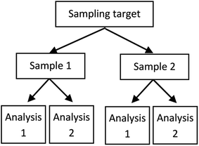
A procedure for the empirical estimation of uncertainty that is often used, and includes the contribution from primary sampling, is known as the duplicate method and often uses a balanced experimental design (Fig. 1).² In this procedure, a number of duplicate samples are taken (in addition to the primary samples) using the same sampling protocol, but with a fresh spatial (or temporal) interpretation of the location of the duplicate sample. Each primary and duplicate sample is then analysed twice.

Fig. 1 Nested balanced experimental design for the duplicate method used in uncertainty estimation. Two samples are acquired using fresh interpretations of the same protocol, and two analyses performed on each.²

Standard deviations are calculated for each of the 3 levels in Fig. 1 by Analysis of Variance (ANOVA). This gives estimates of the standard uncertainty u both at the sampling and analytical levels. The overall MU is obtained by combining the sampling u and analytical u by the sum-of-squares. The expanded relative uncertainty U′ at any level can be expressed as a percentage, with a coverage factor of 2 for approximately 95% confidence, as 2 × 100 × u divided by the concentration value.

Approaches to comparing MU values

Two approaches to uncertainty comparison are discussed and demonstrated in the following example. In the case where variances are estimated from the variance of independent normally distributed samples from the respective populations (note ‘sample’ in this context refers to statistical samples, not physical samples as in Fig. 1), then the preferred method of comparison is to use an F-test. However, the F-test fails to provide accurate results if the data differ significantly from the conditions of normality and independence. If a small deviation from these conditions occurs then an F-test can still be applied. For example, in the case of non-normality where the measurements include a small number of outliers, then variances may have been estimated using robust statistics.³ It may still be reasonable to use an F-test for the comparison, but this will then be an approximation. In other cases it may be possible to use some method of transformation on the data to achieve normality.

Another consideration is that in the particular case of variances estimated using the balanced design described above, the assumption of independence only strictly holds true when comparing variances at the lowest (analytical) level. This is because the variances at the higher levels are calculated by subtracting the variance of the level below. However, it will often be found in practice that variance at the sampling level is much greater than variance at the analytical level, and it may then be reasonable to use an F-test on the combined variances (i.e., on the squares of the MU values) as an approximation.⁴

An alternative to the F-test is to calculate confidence intervals (CIs) for the two uncertainties being compared. Note that here we are talking about CIs of the uncertainties, not CIs of measurement results themselves (or of their mean values). The computer program RANOVA3 (ref. 5) includes an option to calculate CIs on uncertainties for the n × 2 × 2 experimental design introduced earlier (Fig. 1). Discussion and details of the calculations of these CIs can be found in ref. 1 and 6. The CIs can then be compared for overlap. If they do not overlap, then the variances are different with a significance level of p < 0.05. However, this type of comparison has low power as a statistical test. In cases where the CIs do not overlap, we can be confident they are significantly different. However, in cases where they are overlapping, but the degree of overlap is not obviously large, we are unsure whether a significant difference exists or not. It is for this reason that the F-test is to be preferred if the conditions of normality and independence are either fully met, or we have reason to believe that an F-test will be a sufficiently good approximation.⁴

Worked example

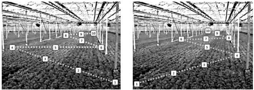
The following study of nitrate concentration in greenhouse grown lettuce⁷ is an example of a situation where we wish to compare the different components of uncertainty that have been estimated for a particular measurement method. Sampling was carried out by collecting 10 lettuce heads from each bay, walking a W-shaped route. Sample duplicates were acquired using the same sampling protocol, but taking an alternative route through the bays (Fig. 2). The 10 heads from each bay were processed to form a composite sample and analysed using high performance liquid chromatography. The results of applying classical and robust ANOVA to the duplicate measurements are shown in Table 1.

Fig. 2 Sampling of lettuce: the protocol (left) specifies taking 10 heads (numbers indicate the order in which the increments were taken) to make a single composite sample from each bay. The duplicate sample (right) was acquired using the same protocol but applying a different route.⁴

Table 1 Classical and robust estimations of the standard deviations (SD) (or uncertainties, u) of the duplicate lettuce data for 8 sampling targets, using the experimental design described in Fig. 1. The lower and upper confidence limits for these values are shown in parentheses (LCL, UCL), as the limits of the CI. ‘Measurement’ (i.e., MU) is the root-sum-square of the standard deviations of ‘Sampling’ and ‘Analytical’

	Between-sampling target (mg kg^−1)	Sampling (mg kg^−1)	Analytical (mg kg^−1)	Measurement (mg kg^−1)
a CI for measurement is an approximation based on linear combinations of variances.^8
SD (or u) classical	556 (0, 1320)	518 (334, 1008)	148 (110, 226)	539 (372,1018)^a
SD (or u) robust	565 (347, 1176)	319 (248, 705)	168 (138, 204)	361 (300, 724)

---

A comparison between the sampling and analytical uncertainty components can indicate where it would be most efficient to allocate resources if it is desired to reduce the overall measurement uncertainty (‘Measurement’ in Table 1). In this case, the CIs of ‘Sampling’ u and ‘Analytical’ u do not overlap in either the classical or the robust results (i.e., 248 to 705 mg kg⁻¹ for robust sampling, does not overlap with 138 to 204 mg kg⁻¹ for the robust analytical). This proves that the sampling uncertainty is significantly larger and clearly dominant, and therefore it could be advantageous to reduce this component of uncertainty, depending on the relative costs of sampling and analysis.

Unfortunately, it is not possible to directly compare the sampling and analytical uncertainties using an F-test. The nested design (see Fig. 1) enables ANOVA to calculate the variances at the target and sample levels by subtracting the mean-square values of the level below (i.e., analytical). Consequently, these two variances do not meet the requirements of independence. However, we can test whether the sampling variance is significantly different from zero using the ratio of the mean-square values at the sampling (MS_S) and analytical (MS_A) level: MS_S/MS_A.⁴ This ratio can be compared with the upper critical value of the F-distribution.⁴

In the following calculations, I is the number of (duplicated) sampling targets (I = 8), J is the number of samples per sampling target (J = 2) and K is the number of analyses per sample (K = 2).

The mean-square ratio can be calculated from the ANOVA results (Table 1) as follows, where s_S and s_A are the robust standard deviations at the ‘Sampling’ and ‘Analytical’ levels, respectively.

Degrees of freedom for the sampling and analytical levels are calculated as I(JS − 1) and IJ(K − 1). From this we can look up a critical value for this ratio F_{crit(0.05,8,16)} = 2.6. The ratio MS_S/MS_A = 8.2 is greater than this critical value, so we can reject the null hypothesis that the sampling variance at the population level (σ_S²) is zero, with 95% confidence for a probability level of α = 0.05.

We can also use the mean-square values to test whether the sampling and analytical variances are significantly different, because in the particular case where the population variances are equal (σ_S² = σ_A²), the distribution of

can be written as

Since MS_S/MS_A = 8.2 is greater than 3 times the critical value (2.6 × 3 = 7.8), the null hypothesis that the sampling variance is not significantly larger than the analytical variance (σ_S² = σ_A²) can also be rejected, indicating that the sampling and analytical variances are significantly different for a chosen probability level of α = 0.05. This supports the previous conclusion (based on CIs) that the sampling uncertainty is dominant.⁴

In general, this approach assumes either that there have been no significant systematic effects contributing to the MU (such as analytical bias), or that they have been corrected for, or included within the estimate of MU.

Conclusion

When comparing uncertainty values the F-test of a variance ratio is the better option, if it can be assumed to be valid. However, there are many common situations where it is not valid. An alternative approach is to compute confidence intervals and compare these for overlap. This is a low power test, which may not matter if the uncertainty estimates being compared are very different. A restricted number of tests can also be carried out using the ratios of the mean-square values from ANOVA, instead of the variances themselves.

The example presented demonstrates a comparison between different components of uncertainty (the ‘Sampling’ and ‘Analytical’ components estimated using the experimental design in Fig. 1). In other situations, where we might wish to compare uncertainties between two different measurement methods, some approximations might be applicable. For example, if we wish to compare two measurement methods where the sampling uncertainty clearly dominates over the analytical uncertainty in both cases, an approximation can then be made using an F-test on the two values of the combined MU. Further details for these other situations are given in ref. 4.

Peter D. Rostron

This Technical Brief was prepared for the Analytical Methods Committee with contributions from members of the AMC Sampling Uncertainty and Statistics Expert Working Groups, and the Eurachem Working Group on Uncertainty from Sampling (both chaired by Michael H. Ramsey), and approved on 4 ^th August 2022.

References

1. Analytical Methods Committee, How reliable is my uncertainty estimate? AMC Technical Brief No. 105, Anal. Methods, 2021, 13, 2728–2731,  10.1039/d1ay90060a.
2. Eurachem/EUROLAB/CITAC/Nordtest/AMC Guide: Measurement uncertainty arising from sampling: a guide to methods and approaches, ed. M. H. Ramsey, S. L. R. Ellison and P. D. Rostron, Eurachem, 2nd edn, 2019, ISBN 978-0-948926-35-8, https://www.eurachem.org/index.php/publications/guides/musamp.
3. Analytical Methods Committee, Robust statistics - how not to reject outliers. Part 1, basic concepts, Analyst, 1989, 114, 1693–1697,  10.1039/AN9891401693.
4. P. D. Rostron, T. Fearn and M. H. Ramsey, Comparing uncertainty values – Are they really different?, Accredit. Qual. Assur., 2022, 27, 133–142,  DOI:10.1007/s00769-022-01501-2.
5. Analytical Methods Committee (2020) RANOVA3 computer program available from https://www.rsc.org/Membership/Networking/InterestGroups/Analytical/AMC/Software/index.asp.
6. P. D. Rostron, T. Fearn and M. H. Ramsey, Confidence intervals for robust estimates of measurement uncertainty, Accredit. Qual. Assur., 2020, 25, 107–119,  DOI:10.1007/s00769-019-01417-4.
7. J. A. Lyn, I. M. Palestra, M. H. Ramsey, A. P. Damant and R. Wood, Modifying uncertainty from sampling to achieve fitness for purpose: a case study on nitrate in lettuce, Accredit. Qual. Assur., 2007, 12, 67–74,  DOI:10.1007/s00769-006-0239-0.
8. C. A. Graybill and C.-M. Wang, Confidence intervals on nonnegative linear combinations of variances, J. Am. Stat. Assoc., 1980, 75, 869–873,  DOI:10.2307/2287174.

---